Compound Poisson Statistics and Models of Clustering of Radiation Induced DNA Double Strand Breaks.

Abstract

According to the experimental evidence damage induced by densely ionizing radiation in mammalian cells is distributed along the DNA molecule in the form of clusters. The most critical constituent of DNA damage are double-strand breaks (DSBs) which are formed when the breaks occur in both DNA strands and are directly opposite or separated by only a few base pairs. The paper discusses a model of clustered DSB formation viewed in terms of compound Poisson process along with the predictive assay of the formalism in application to experimental data.
PACS numbers: 87.10.+e, 05.40.+j

I Introduction

In living cells subjected to ionizing radiation many chemical reactions are induced leading to various biological effects such as mutations, cell lethality or neoplastic transformation [1, 2]. The most important target for radiation induced chemical transformation where these changes can be critical for cell survival is DNA distributed within the cell’s nucleus. Nuclear DNA is organized in a hierarchy of structures which comprise the cellular chromatin. The latter is composed of DNA, histones and other structural proteins as well as polyamines. Organization of DNA within the chromatin varies with the cell type and changes as the cell progresses through the cell cycle. Ionizing radiation produces variety of damage to DNA including base alterations and single- and double strand breaks (DSBs) in the sugar-phosphate backbone of the molecule [1, 3]. Single strand breaks (SSBs) are efficiently repaired with high fidelity and probably contribute very little to the loss of function of living cells. On the other hand, DSBs are believed to be the critical lesions produced in chromosomes by radiation; interaction between DSBs can lead to cell killing, mutation or carcinogenesis. The purpose of theoretical modeling of radiation action [4]–[7] is to describe qualitatively and quantitatively the results of radiobiological effects at the molecular, chromosomal and cellular level. The basic consideration in such an approach must be then descriptive analysis of breaks in DNA caused by charged particle tracks and by the chemical species produced.
Production of DSBs in intracellular DNA can be studied by use of the pulsed field gel electrophoresis (PFGE) [8] in which the gel electrophoresis is applied to elute high molecular weight DNA fragments from whole cellular DNA embedded in an organic gel (agarose). Two main approaches of this technique are usually applied. One is the measurement of the fraction of DNA leaving the well in PFGE, i.e. the amount of DNA smaller than a certain cutoff size defined by the electrophoretic conditions. This method has proven to be very sensitive, allowing reproducible measurements at relatively low doses. The second approach is to describe fragment-size distributions obtained after irradiation as a function of dose, taking advantage of the property of PFGE to separate DNA molecules based on how quickly they reorient in a switching (pulsed) electrical field. The major goal of the experiments is to quantify number of induced DSBs based on changes in the amount of DNA or the average fragment size in response to dose. In both cases data obtained are related to average number of DSBs. To analyze the data, the formalism describing random depolarization of polymers of finite size is usually adopted [9, 10] giving very well fits to experimental results with X-ray induced DNA fragmentation. In contrast to the findings for sparsely ionizing irradiation (X and $\gamma$ rays) characterized by low average energy deposition per unit track length (linear energy transfer, LET$\approx$ 1 keV/$\mu$m), the densely ionizing (high LET) particle track is spatially localized [2, 11]. In effect, multiplicity of ionizations within the track of heavy ions can produce clusters of DSBs on packed chromatin [13]. The formation of clusters depends on chromatin geometry in the cell and radiation track structure.
DSBs multiplicity and location on chromosomes may determine the distribution of DNA fragments detected in PFGE experiments. Modeling DNA fragment-size-distributions provides then a tool which allows to elucidate experimentally observed frequencies of fragments. Even without detailed information on the geometry of chromatin, models of radiation action on DNA can serve with some predictive information concerning measured DNA fragment-size-distribution. The purpose of the present paper is to discuss a model which can be used in analysis of DNA fragment-size- distribution after heavy ion irradiation. The background of the model is the Poisson statistics of radiation events which lead to formation of clusters of DNA damage. The formation of breaks to DNA can be then described as the generalized or compound Poisson process for which the overall statistics of damage is an outcome of the random sum of random variables (Section 2). Biologically relevant distributions are further derived and used (Section 3) in description of fragment size distribution in DNA after irradiation with heavy ions. Practical use of the formalism is discussed by fitting the distributions to experimental data.

II Random sums of random variables and compound Poisson distributions

Consider [14, 15] a sum $S_{N}$ of $N$ independent random variables $X$

$$S_{N}=\sum_{i=1}^{N}X_{i}$$ (1)

where $N$ is a random variable with a probability generating function $g(s)$

$$g(s)=\sum^{\infty}_{i=0}g_{i}s^{i}$$ (2)

and $X_{i}$ are i.i.d. variables (independent and sampled from the same distribution) whose generating function $f(s)$ is

$$f(s)=\sum_{j=1}^{\infty}f_{j}s^{j}$$ (3)

By use of the Bayes rule of conditional probabilities the probability that $S_{N}$ takes value $j$ can be then written as

$$P(S_{N}=j)\equiv h_{j}=\sum^{\infty}_{n=0}P(S_{N}=j|N=n)P(N=n)$$ (4)

For fixed value of $n$ and by using the statistical independence of $X_{i}$’s, the sum $S_{N}$ has a probability generating function $F(s)$ being a direct product of $f(s)$, i.e. $F(s)=f(s)^{n}=\sum^{\infty}_{j=0}F_{j}s^{j}$ from which it follows that $P(S_{N}=j|N=n)=F_{j}$. The formula (4) leads then to the compound probability generating function of $S_{N}$ given by

$$h(s)=\sum^{\infty}_{j=0}h_{j}s^{j}=$$ (5)

$$=\sum^{\infty}_{j=0}\sum^{\infty}_{n=0}F_{j}g_{n}s^{j}=$$ (6)

$$=\sum^{\infty}_{n=0}g_{n}{f(s)}^{n}\equiv g\{f(s)\}$$ (7)

Conditional expectations rules can be used to determine moments of a random sum. Given $E[N]=\nu$, $E[X_{i}]=\mu$, $Var[N]=\tau^{2}$ and $Var[X_{i}]=\sigma^{2}$, the first and the second moment of the random sum $S_{N}$ are

$$E[S_{N}]=\mu\nu,\qquad Var[S_{N}]=\nu\sigma^{2}+\mu^{2}\tau^{2}$$ (8)

The above compound distribution is describing “clustered statistics” of events grouped in a number $N$ of clusters which itself has a distribution. As such, it is sometimes described in literature [16] as “mixture of distributions”. Out of many interesting biological applications of compound distributions [17]-[20], a special class constitute Poisson point processes which can be also analyzed in terms of random sums with Poisson distributed random events $N$. It can be shown that a mixture of Poisson distributions resulting from using any unimodal continuous function $f(\lambda)$ is a unimodal discrete distribution. It is not so, however, in case of unimodal discrete mixing. In particular, mixtures of Poisson-Poisson or Poisson-binomial, known in literature as Neyman distributions [21] can exhibit strongly multinomial character. By virtue of the above formalism and by using the formulae (7) , the generating function of the compound Poisson-Poisson distribution is:

$$g=\exp(-\lambda(1-f(s)))$$ (9)

where the random variables $X_{i}$ are distributed according to a Poisson law

$$f(s)=\exp(-\mu+\mu s)$$ (10)

and the total $S_{N}$ is a random variable with a compound Poisson-Poisson (Neyman type A) distribution:

$$P(S_{N}=x)\equiv P(x;\mu,\lambda)=\sum_{N=0}^{\infty}\frac{(N\mu)^{x}e^{-N\mu}}{x!}\frac{\lambda^{N}e^{-\lambda}}{N!}$$ (11)

for which the mean and variance are given by

$$E[x]=\mu\lambda,\qquad Var[x]=\lambda\mu(1+\mu)$$ (12)

The resulting distribution can be interpreted as a mixture of Poisson distribution with parameter $N\mu$ where $N$ (number of clusters) is itself Poisson distributed with parameter $\lambda$. Figures 1,2 present function (11) for two various sets of parameters $\lambda,\mu$.

The compound Poisson distribution (CPD) has a wide application in ecology, nuclear chain reactions and queing theory [4, 19, 20, 21]. It is sometimes known as the distribution of a “branching process” and as such has been also used to describe radiobiological effects of densely ionizing radiation in cells [17, 22, 23, 24]. When a single heavy ion crosses a cell nucleus, it may produce DNA strand breaks and chromatin scissions wherever the ionizing track structure overlaps chromatin structure. The multiple yield of such lesions depends on the radial distribution of deposited energy and on the microdistribution of DNA in the cell nucleus. The latter and the geometry of DNA coiling in the cell nucleus determine number of crossings, the “primary” incidents leading to DSBs production. By assuming for a given cell line, a “typical” average number $n$ of possible crossings per particle traversal, the distribution of the number of chromatin breaks $i$ can be modelled by a binomial law:

$$P(i|n)={n\choose i}p^{i}q^{(n-i)}$$ (13)

where $p$ is a probability that a chromatin break occurs at each particle crossing (and $q$ is the probability that it does not). The overall probability that $i$ lesions will be observed after $m$ independent particles traversed the nucleus is given by [4]

$${\bf P}(i|\sigma,F,n)=\sum^{\infty}_{m=1}\frac{(nm)!p^{i}q^{(nm-i)}(\sigma F)^{m}e^{-\sigma F}}{i!(nm-i)!m!}$$ (14)

which is a compound Neyman type B distribution obtained as a random Poisson sum of binomially distributed i.i.d variables. In the above presentation the average number of particles crossing the cell nucleus $\lambda$ is proportional to the absorbed energy (dose) and given by a product $\lambda=\sigma F$ of particle fluence $F$ and nuclear cross section $\sigma$.

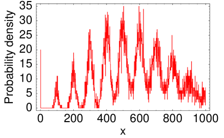
FIG. 1.: Simulated probability density function for the Neyman-type A distribution (11) with $\lambda=6,\mu=100$ for $N=10000$ points. Note the finite value at $x=0$ corresponding to $P(0;\mu,\lambda)$.

Aggregation of observed cellular damage potentially leads to the phenomenon of “overdispersion”– that is, the variance of the aggregate may be larger than Poisson variance yielding “relative variance” $Var_{rel}=Var[S_{N}]/E[S_{N}]$ larger than 1. Assuming thus the Poisson statistics of radiative events, for any distribution of lesions per particle traversal, the condition for overdispersion can be easily rephrased in terms of (8)

$$Var[X_{i}]/E[X_{i}]+E[X_{i}]<1$$ (15)

If no repair process is involved in diminishing number of initially produced lesions, the surviving fraction of cells can be estimated from formula eq.(14) as a zero class of the initial distribution, i.e. the proportion of cells with no breaks

$${\bf P}_{N}(0|\sigma,F,n)=\sum^{\infty}_{m=1}\frac{(nm)!q^{nm}(\sigma F)^{m}e^{-\sigma F}}{(nm)!m!}=$$ (16)

$$=\exp[-\sigma F(1-q^{n})]$$ (17)

which differs by a factor $(1-q^{n})$ in the exponent from the surviving fraction for a Poisson distribution:

$${\bf P}_{P}(0|\sigma,F,n)=\exp[-\sigma F]=\exp[-E[i]]$$ (18)

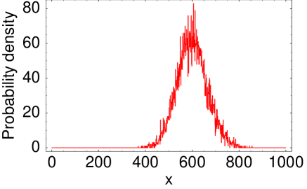
FIG. 2.: Simulated probability density function for the Neyman-type A distribution (11) with $\lambda=100,\mu=6$ for $N=10000$ points

III DNA fragments distribution generated by irradiation: statistical model.

DNA double stranded molecules in a size range from a few tenths of kilobase pairs to several megabase pairs can be evaluated by the PFGE technique. Randomly distributed DSBs are detected as smears of DNA fragments. The DNA mobility mass distribution may be transformed into a fragment length distribution using a calibration curve. It is obtained by relating migration distance of DNA within the gel to molecular length with the aid of size markers loaded on the same gel [25]. To interpret the experimental material one needs to relate percentage of fragments in defined size ranges to number of induced DSBs. For that purpose several models have been derived, mainly based on the description of random depolarization of polymers of finite size [9, 10, 26]. Although the models give satisfactory prediction of size-frequency distribution of fragments after sparsely ionizing radiation (i.e for X-rays and $\gamma$), they generally fail to describe the data after densely ionizing radiation [13, 25]. The experiments with heavy ions demonstrate that after exposure to densely ionizing particles gives rise to substantially overdispersed distribution of DNA fragments which indicates the occurrence of clusters of damage. The following analysis presents a model which takes into account formation of aggregates of lesions after heavy ion irradiation.
Fragment distribution in PFGE studies is measured by use of fluorescence technique or radioactive labeling with the result being the intensity distribution. The generated signal is proportional to the relative intensity distribution of DNA fragments and can be expressed as

$$I(x)=xD(x)$$ (19)

with

$$D(x)=\sum_{j=0}^{\infty}D(x|j)P(j;\mu,\lambda)$$ (20)

where $D(x|j)$ stands for the density of fragments of length $x$ provided $j$ DSBs occur on the chromosome of size $S$. Frequency distribution of the number of DSBs is assumed here in the form of CPD (11) with parameters $\mu$ and $\lambda$ representing average number of breaks produced by a single particle traversal and average number of particle traversals, respectively. The “broken-stick” distribution [27, 26] for $j$ breaks on a chromosome of size $S$ yields a density of fragments of size $x$:

$$D(x|j)=\delta(x-S)+2j\frac{1}{S}(1-\frac{x}{S})^{j-1}+$$ (21)

$$+j(j-1)\frac{1}{S}(1-\frac{x}{S})^{j-1}$$ (22)

where the first two terms describe contributions from the edge fragments of the chromosome and the third term describes contribution from the internal fragments of length $x<S$. The first term applies to the situation when $j=0$; the edge contribution can be understood by observing that the first and the $j+1$ fragment have the same probability of being size $x$. Direct summation in formula (20) leads to

$$D_{N}(x)=\exp(-\lambda(1-e^{-\mu}))\delta(x-S)+$$ (23)

$$+\frac{2\lambda\mu}{S}\exp(-\mu\frac{x}{S}+\lambda(e^{-\mu\frac{x}{S}}-1))+$$ (24)

$$+e^{-\lambda}(1-\frac{x}{S})\frac{\mu^{2}\lambda}{S}(1+\lambda e^{-\mu\frac{x}{S}})\exp(-\mu\frac{x}{S}+\lambda e^{-\mu\frac{x}{S}})$$ (25)

for Neyman distribution of number of breaks $j$ and to

$$D_{P}(x)=\Lambda\exp(-\Lambda\frac{x}{S})(2+\Lambda-\Lambda\frac{x}{S})$$ (26)

for a Poisson distribution with parameter $\Lambda$. Integration of $I(x)$ (eq.(3.1)) from 0 to some average (marker) size $X^{*}$ and division by $S$ yields the relative fraction of DNA content. For $\lambda>>1$ and $\mu<<1$, the Neyman-type A distribution converges to a simple Poisson. In such a case, simplified expression (25) leads to results known in literature as “Blöcher formalism” [9, 10, 26] which describes well the DNA content in probes irradiated with X– and $\gamma$–rays.

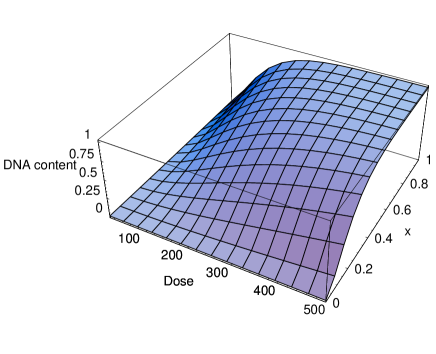
FIG. 3.: Distribution of DNA content (integrated eq.(19)) as a function of the dose and fragment size for $S=245Mbp,\mu=5$. The fragments length is in Mbp units.

Figure 3 presents predicted dose-response curves for the model. The amount of DNA content is shown in function of dose and fragment size. In calculation, the parameter $S=245$ mega base pairs has been used which is the mean chromosome size for Chinese hamster cells, the cell line for which experimental data are displayed in Figure 4.
The increase in multiplicity of DSBs produced per one traversal of a particle leads to pronounced increase in production of shorter fragments which is illustrated in the shift of the peak intensity towards smaller $x$ values.

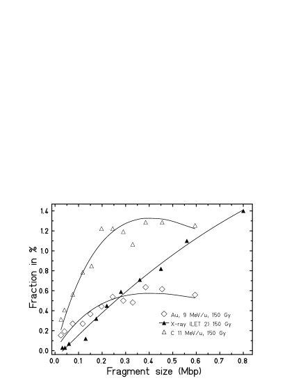
FIG. 4.: Fraction of DNA content observed experimentally within the range of sizes 0.1-1.0 Mbp. Data show higher probability of producing short fragments after irradiation with particles than for sparsely ionizing radiation at comparative dose. Lines represent the best fit to eq.(3.1) by use of $D_{N}(x)$ function for heavy ions (Au: $\lambda=3\times 10^{-3},\mu=6\times 10^{2}$ ; C: $\lambda=6\times 10^{-3},\mu=6\times 10^{2}$) and $D_{P}(x)$ for X-rays ($\Lambda=0.85$).

IV Spatial Clustering of Breaks and Non-Poisson statistics.

Clustering of breakage events can be viewed as the process leading to non-exponential “spacing” between subsequent events, similar to the standard analysis of level repulsion in spectra of polyatomic molecules and complex nuclei. For a random sequence, the probability that a DSB will be in the infinitesimal interval

$$(X+x,X+x+dx)$$ (27)

proportional to $dx$ is independent of whether or not there is a break at $X$. This result can be easily changed by using the concept of breaks “repulsion’. Given a break at $X$, let $P(x)dx$ be the probability that the next break ($x\geq 0$) be found in the interval $(X+x,X+x+dx)$. We then have for the nearest-neighbour spacing distribution of breaks the following formula:

$$P(x)dx=Prob(1\in dx|0\in x)Prob(0\in x)$$ (28)

where $Prob(n\in dx|m\in x)$ is the conditional probability that the infinitesimal interval of length $dx$ contains $n$ breaks wheras that of length $x$ contains $m$ of those. The first term on the right-hand side of the above equation is $dx$ times a function of $x$ which we denote by $r(x)$, depending explicitly on the choices 1 and 0 of the discrete variables $n$ and $m$. The second term is given by the probability that the spacing is larger than $x$:

$$\int^{\infty}_{x}P(y)dy$$ (29)

Accordingly, one obtains

$$P(x)=r(x)\int^{\infty}_{x}P(y)dy,$$ (30)

whose solution can be easily found to be

$$P(x)=Cr(x)\exp(-\int^{x}r(y)dy)$$ (31)

where $C$ is a constant. The Poisson law, which reflects lack of correlation between breaks, follows if one takes $r(x)=\lambda$, where $\lambda^{-1}$ is the mean spacing between DSBs. If choosing on the other hand

$$r(x)=\lambda x^{\lambda-1}$$ (32)

i.e. by assuming clustering of points (DSBs) along a line, one ends up with the Weibull density. The constants $C$ and $\lambda$ can then be determined from appropriate conditions, e.g.

$$\int P(x)dx=1,$$ (33)

and

$$\int xP(x)dx=\lambda^{-1}$$ (34)

One then finds that

$$P(x)=\lambda e^{-\lambda x}$$ (35)

for the Poisson distribution and

$$P(x)=\lambda x^{\lambda-1}\exp(-x^{\lambda})$$ (36)

for the Weibull analogue. Note that the above density can be derived as a generalization of the law eq.(35): the Weibull density can be obtained as the density of random variable $y=x^{1/\lambda}$ with $x$ being an exponential random variable. For $\lambda\geq 1$, the Weibull distribution is unimodal with a maximum at point $x_{m}=(1-\lambda^{-1})^{\lambda^{-1}}$. In this one easily recognizes for $\lambda=2$ the spacing distribution of the Wigner law. The latter displays “repulsion” of spacing, since $P(0)=0$, in contrast to the Poisson case which gives maximum at $x=0$. Fractional exponent $\lambda<1$ describes, on the other hand, enhanced frequency of short spacings which, in fact, matches better experimental data for heavy ions(cf. Figure 4). The above analysis brings also similarities with random walks [29, 30] where symmetry breaking transition manifests itself as a change in the spectral spacing statistics of decay rates. In such cases, the statistics of events of interest deviates, as a counting process, from the regularity of Poisson process, for which the subsequent event arrivals are spaced with a constant mean $\lambda^{-1}$. The clustered statistics of breakage can be thus viewed as a (fractal) random walk or a cumulative distribution of a random sum of random variables eq.(2.1). The problem of characterizing the limit distribution for such cases with underlying “broad” distributions $g(x)$ of $X_{i}$ has been studied extensively in mathematical literature [32] and has been solved with classification of the possible limit distributions provided that requirement of “stability” is fulfilled under convolution. Following the definition, the distribution $g(x)$ is stable, if for any $N$ there exist constants $c_{N}>0$ and $d_{N}$ such that $S_{N}$ has the same density as the variable $y=c_{N}X_{i}+d_{N}$. The stability condition can be rephrased in terms of the canonical representation given by a form of the characteristic function (i.e. the Fourier transform $g(k)$) of stable distributions [33, 32]

$$\ln g(k)=i\gamma k-C|k|^{\lambda}[1-i\omega\beta sign(k)]$$ (37)

where $\gamma$ is real, $0\leq\lambda\leq 2$, $\omega$ is real and $|\omega|\leq tan(\pi\lambda/2)|$. The cases relevant for biological modelling are covered by $1\leq\lambda\leq 2$ (stable distributions have no variance if $\lambda<2$ and no mean if $\lambda<1)$. In particular, positivity of steps in the random walk modelled by eq.(2.1) allows for $g(k)=\exp[-C|k|^{\lambda}]$ which gives asymptotically $g(x)\approx x^{-\lambda-1}$. Probability distribution that $x\geq z$ satisfies then $f(z)\approx z^{-\lambda}$ for $z\rightarrow\infty$. The resulting distribution is “self-similar” in the sense that rescaling $z$ to $Az$ and $f(z)$ to $A^{-\lambda}f(z)$ does not change the power law distribution. In other words, the number of realizations larger than $Az$ is $A^{-\lambda}$ times the number of realizations larger than $z$. The power-law probability distribution function describes then the same proportion of shorter and larger fragments whatever size is discussed within the power law range. For $\lambda=1/2,C=1,\omega=1$ the form of Lèvy-Smirnov law is recovered

$$g(x)=(2\pi)^{-1/2}x^{-3/2}e^{-\frac{1}{2x}}$$ (38)

The probability density eq.(38) has a simple interpretation as the limiting law of return times to the origin for a one-dimensional symmetrical random walk and as such has been also used to describe the fragment size distribution of a one dimensional polymer [31, 34]. In the problems related to polymer fragmentation induced by irradiation, the approach based on a random walk with fluctuating number of steps (or, equivalently, on a point proceses model with a clustered statistics of waiting times) is a legitimate one as it can comprise the natural randomness of primary events (i.e. particle hits of biological target) and secondary induction of multiple (clustered) lesions. Further investigations in this field should lead to better understanding of possible emergence of power-law distributions of larger fragments on kbp and Mbp scales.

V Conclusions

An existing substantial evidence demonstrates that exposure to densely ionizing charged particles gives rise to overdispersed distribution of chromatin breaks and DNA fragments which is indicative of clustered damage occuring in irradiated cells. The clustering process can be expressed for any particular class of events such as ionizations or radical species formation and is a consequence of energy localization in the radiation track. Chromosomal aberrations expressed in irradiated cells are formed in process of misrejoining of fragments which result from production of double-strand breaks in DNA. The location of double-strand breaks along chromosomes determines DNA fragment-size distribution which can be observed experimentally. The task of stochastic modeling is then to relate parameters of such distributions to relevant quantities describing number of induced DSBs. Application of the formalism of clustered breakage offers thus a tool in evaluation of the radiation respone of DNA fragment-size distribution and assessment of radiation induced biological damage.

Acknowledgements.
E.G-N acknowledges partial support by KBN grant 2PO3 98 14 and by KBN–British Council collaboration grant C51.

REFERENCES

REFERENCES

- [1] E.L. Alpen, Radiation Biophysics, (Academic Press, San Diego, 1998).
- [2] G.Kraft, Nucl. Science Appl. 1 (1987) 1.
- [3] C. Von Sonntag, The Chemical Basis of Radiation Biology, (Taylor and Francis, London, 1987); J.F. Ward, Int. J. Radiat. Biol. 66 (1994) 427.
- [4] C.A. Tobias, E. Goodwin and E. Blakely, in Quantitative Mathematical Models in Radiation Biology, J. Kiefer, ed., Springer Verlag, Berlin 1988, p.135.
- [5] P.J. Hahnfeldt, R.K. Sachs and L.R. Hlatky, J. Math. Biol. 30 (1992) 493.
- [6] A.Chatterjee and W. Holley, Int. J. Quant. Chem. 391 (1991) 709.
- [7] R. Sachs, D.J. Brenner, P.J. Hahnfeldt and R. Hlatky, Int. J. Radiat. Biol. 74 (1998) 185.
- [8] G. Iliakis, D. Blöcher, L. Metzger and G. Pantelias, Int. J. Radiat. Biol. 59 (1991) 927.
- [9] E.W. Montroll and R. Simha, J. Chem. Phys. 8 (1940) 721.
- [10] D. Blöcher, In.J. Radiat. Biol. 57 (1990) 7.
- [11] M. Krämer and G. Kraft, Rad. Env. Biophysics 33 (1994) 91.
- [12] G. Taucher-Scholz and G. Kraft, Rad. Res. 151 (1999) 595
- [13] M. Löbrich, P. Cooper and B. Rydberg, Int. J. Radiat. Biol. 70 (1996) 493; H.C. Newman, K.M. Prise, M. Folkard and B.D. Michael, ibid 71 (1997) 347; E. Höglund, E. Blomquist, J. Carlsson and B. Sternlöw, ibid 76 (2000) 539.
- [14] N.G. Van Kampen, Stochastic Processes in Physics and Chemistry, (North Holland, Amsterdam, 1981).
- [15] A. Papoulis, Probability, Random Variables and Stochastic Processes, (McGraw-Hill, Tokyo, 1981).
- [16] M. Kendall and A. Stuart, The Advanced Theory of Statistics, Charles Griffin & Co., London, 1977.
- [17] N. Goel and N. Richter-Dyn, Stochastic Processes in Biology, (Academic Press, New York, 1974).
- [18] T. Maruyama, Mathematical Modeling in Genetics, (Springer Verlag, Berlin, 1981).
- [19] A.T. Bharucha-Reid, Elements of the Theory of Markov Processes and Their Applications, (Dover Publications, New York, 1988).
- [20] S. Karlin and H. Taylor, First Course in Stochastic Processes, (Academic Press, New York, 1976).
- [21] J. Neyman, Am. Math. Stat. 10 (1939) 35.
- [22] N. Albright, Radiat. Res. 118 (1989) 1.
- [23] E. Gudowska-Nowak, S. Ritter, G. Taucher-Scholz and G. Kraft, Acta Phys. Pol. 31B (2000) 1109.
- [24] E. Nasonova, E. Gudowska-Nowak, S. Ritter and G. Kraft, Int. J. Radiat. Biol., (2000), in press.
- [25] J. Heilmann, G. Taucher-Scholz and G.Kraft, Int. J. Radiat. Biol., 68 (1995) 153; G. Taucher-Scholz and G. Kraft, Rad. Res. 151 (1999) 595
- [26] T. Radivoyevitch and B. Cedervall, Electrophoresis 17 (1996) 1087.
- [27] P.J. Flory Statistical Mechanics of Chain Molecules (Interscience, New York, 1969).
- [28] G. Van den Engh, R. Sachs and B. Trask, Science 257 (1986) 1410.
- [29] P. Alpatov and L.E. Reichl, Phys. Rev. E 52 (1995) 4516.
- [30] D.R. Nelson and N.M. Shnerb, Phys. Rev. E. 58 (1998) 1384.
- [31] G.H. Weiss and R.J. Rubin, Adv. Chem. Phys. 52 (1983) 363.
- [32] V.M. Zolotarev One-dimensional Stable Distributions, (American Mathematical Society, Providence, 1986)
- [33] B.V. Gnedenko and A.N. Kolmogorov Limit Distributions for Sums of Independent Random Variables, (Addison Wisley MA 1954)
- [34] A.L. Ponomarev and R.K. Sachs, Bioinformatics 15 (1999) 957.