Fast and stable method for simulating quantum electron dynamics

Abstract

A fast and stable method is formulated to compute the time evolution of a wavefunction by numerically solving the time-dependent Schrödinger equation. This method is a real space/real time evolution method implemented by several computational techniques such as Suzuki’s exponential product, Cayley’s form, the finite differential method and an operator named adhesive operator. This method conserves the norm of the wavefunction, manages periodic conditions and adaptive mesh refinement technique, and is suitable for vector- and parallel-type supercomputers. Applying this method to some simple electron dynamics, we confirmed the efficiency and accuracy of the method for simulating fast time-dependent quantum phenomena.

I Introduction

There are many computational method of solving the TD-Schrödinger equation numerically. Conventionally, a wavefunction has been represented as a linear combination of plane waves or atomic orbitals. However, these representations entail high computational cost to calculate the matrix elements for these bases. The plane wave bases set is not suitable for localized orbitals, and the atomic orbital bases set is not suitable for spreading waves. Moreover, they are not suitable for parallelization, since the calculation of matrix elements requires massive data transmission among processors.

To overcome those problems, some numerical methods adopted real space representation[1, 2, 3, 4]. In those methods, a wavefunction is descritized by grid points in real space, and with them some dynamic electron phenomena were simulated successfully [6, 7, 8].

Among these real space methods, a method called Cayley’s form or Crank-Nicholson scheme is known to be especially useful for one-dimensional closed systems because this method conserves the norm of the wavefunction exactly and the simulation is rather stable and accurate even in a long time slice. These characteristics are very attractive for simulations over a long time span. Unfortunately, this method is not suitable for two- or three-dimensional systems. This problem is fatal for physically meaningful systems. Though there are many other computational methods that can manage two- or three-dimensional systems, these methods also have disadvantages.

In the present work, we have overcome the problems associated with Cayley’s form and have formulated a new computational method which is more efficient, more adaptable and more attractive than any other ordinary methods.

In our method, all computations are performed in real space so there is no need of using Fourier transform. The time evolution operator in our method is exactly unitary by using Cayley’s form and Suzuki’s exponential product so that the norm of the wavefunction is conserved during the time evolution. Stability and accuracy are improved by Cayley’s form so we can use a longer time slice than those of the other methods. Cayley’s form is a kind of implicit methods, this is the key to the stability, but implicit methods are not suitable for periodic conditions and parallelization. We have avoided these problems by introducing an operator named adhesive operator. This adhesive operator is also useful for adaptive mesh refinement technique.

Our method inherits many advantages from many ordinary methods, and yet more improved in many aspects. With these advantages, this method will be useful for simulating large-scale and long-term quantum electron dynamics from first principles.

In section II, we formulate the new method step by step. In section III, we apply it to some simulations of electron dynamics and demonstrate its efficiency. In section IV, we draw some conclusions.

II Formulation

In this section, we formulate the new method step by step from the simplest case to complicated cases. Throughout this paper, we use the atomic units $\hbar=1,\,m=1,\,e=1$.

A One-dimensional closed free system

For the first step, we consider a one-dimensional closed system where an electron moves freely but never leaks out of the system. The TD-Schrödinger equation of this system is simply given as

$${\rm i}\frac{\partial\psi(x,t)}{\partial t}=-\frac{\partial_{x}^{2}}{2}\,\psi(x,t)\ .$$ (1)

The solution of Eq. (1) is analytically given by an exponential operator as

$$\psi(x,t+\Delta{t})=\exp{\Bigl{[}{\rm i}\Delta{t}\frac{\partial_{x}^{2}}{2}\Bigr{]}}\ \psi(x,t)\ ,$$ (2)

where $\Delta{t}$ is a small time slice. By using Eq. (2) repeatedly, the time evolution of the wavefunction is obtained.

An approximation is utilized to make a concrete form of the exponential operator. We have to be careful not to destroy the unitarity of the time evolution operator, otherwise the wavefunction rapidly diverges. We adopted Cayley’s form because it is unconditionally stable and accurate enough. Cayley’s form is a fractional approximation of the exponential operator given by

$$\exp{\Bigl{[}{\rm i}\Delta{t}\frac{\partial_{x}^{2}}{2}\Bigr{]}}\simeq\frac{1+{\rm i}\Delta{t}\partial_{x}^{2}/4}{1-{\rm i}\Delta{t}\partial_{x}^{2}/4}\ .$$ (3)

It is second-order accurate in time. By substituting Eq. (3) for Eq. (2) and moving the denominator onto the left-hand side, the following basic equation is obtained:

$$\Bigl{[}1-{\rm i}\frac{\Delta{t}}{2}\frac{\partial_{x}^{2}}{2}\Bigr{]}\ \psi(x,t+\Delta{t})=\Bigl{[}1+{\rm i}\frac{\Delta{t}}{2}\frac{\partial_{x}^{2}}{2}\Bigr{]}\ \psi(x,t)\ .$$ (4)

This is identical with the well-known Crank-Nicholson scheme. The wavefunction is descritized by grid points in real space as

$$\psi_{i}(t)=\psi(x_{i},t)\ ;\qquad x_{i}=i\Delta{x},\quad i=0,\cdots,N-1$$ (5)

where $\Delta{x}$ is the span of the grid points. We approximate the spatial differential operator by the finite difference method (FDM). Then Eq. (4) becomes a simultaneous linear equation for the vector quantity $\psi_{i}(t+\Delta{t})$. For example, in a system with six grid points, Eq. (4) is approximated in the following way:

$$\left[\begin{array}[]{cccc}A&-1&0&0\\ -1&A&-1&0\\ 0&-1&A&-1\\ 0&0&-1&A\end{array}\right]\left[\begin{array}[]{c}\psi_{1}(t+\Delta{t})\\ \psi_{2}(t+\Delta{t})\\ \psi_{3}(t+\Delta{t})\\ \psi_{4}(t+\Delta{t})\end{array}\right]\\ =\left[\begin{array}[]{cccc}B&1&0&0\\ 1&B&1&0\\ 0&1&B&1\\ 0&0&1&B\end{array}\right]\left[\begin{array}[]{c}\psi_{1}(t)\\ \psi_{2}(t)\\ \psi_{3}(t)\\ \psi_{4}(t)\end{array}\right]$$ (6)

In the above,

$$A\equiv-4{\rm i}\frac{\Delta{x}^{2}}{\Delta{t}}+2\ ,\ B\equiv-4{\rm i}\frac{\Delta{x}^{2}}{\Delta{t}}-2\$$ (7)

and $\psi_{0}$ and $\psi_{5}$ are fixed at zero due to the boundary condition.

It is easy to solve this simultaneous linear equation because the matrix appearing on the left-hand side is easily decomposed into the LU form as

$$\left[\begin{array}[]{cccc}u_{1}^{-1}&0&0&0\\ -1&u_{2}^{-1}&0&0\\ 0&-1&u_{3}^{-1}&0\\ 0&0&-1&u_{4}^{-1}\end{array}\right]\left[\begin{array}[]{cccc}1&-u_{1}&0&0\\ 0&1&-u_{2}&0\\ 0&0&1&-u_{3}\\ 0&0&0&1\end{array}\right]\\ \times\left[\begin{array}[]{c}\psi_{1}(t+\Delta{t})\\ \psi_{2}(t+\Delta{t})\\ \psi_{3}(t+\Delta{t})\\ \psi_{4}(t+\Delta{t})\end{array}\right]=\left[\begin{array}[]{c}b_{1}(t)\\ b_{2}(t)\\ b_{3}(t)\\ b_{4}(t)\end{array}\right]$$ (8)

Here $b_{i}$ and $u_{i}$ are auxiliary vectors defined as below

$$b_{i}(t) \equiv\psi_{i-1}(t)+B\psi_{i}(t)+\psi_{i+1}(t),$$ (9)

$$u_{i} \equiv 1/(A-u_{i-1}),\quad u_{0}\equiv 0$$ (10)

The auxiliary vector $u_{i}$ is determined in advance, and it is treated as a constant vector in Eq. (10). $26N$ floating operations are heeded to solve Eq. (10); here $N$ is the number of the grid points in the system, about twice that of the Euler method. Unlike the Euler method, it exactly conserves the norm because the matrices in Eq. (6) are unitary. Moreover, the expected energy is conserved because the time evolution operator commutes with the Hamiltonian in this case.

B Three-dimensional closed free system

It is easy to extend this technique to a three-dimensional system. The formal solution of the TD-Schrödinger equation in a three-dimensional system is given by an exponential of the sum of three second differential operators as

$$\psi({\bf r},t+\Delta{t})=\exp{\Bigl{[}{\rm i}\Delta{t}\Bigl{(}\frac{\partial_{x}^{2}}{2}+\frac{\partial_{y}^{2}}{2}+\frac{\partial_{z}^{2}}{2}\Bigr{)}\Bigr{]}}\ \psi({\bf r},t)\ .$$ (11)

These differential operators in Eq. (11) are commutable among each other, so the exponential operator is exactly decomposed into a product of three exponential operators:

$$\psi({\bf r},t+\Delta{t})=\exp{\Bigl{[}{\rm i}\Delta{t}\frac{\partial_{x}^{2}}{2}\Bigr{]}}\ \exp{\Bigl{[}{\rm i}\Delta{t}\frac{\partial_{y}^{2}}{2}\Bigr{]}}\ \\ \times\exp{\Bigl{[}{\rm i}\Delta{t}\frac{\partial_{z}^{2}}{2}\Bigr{]}}\ \psi({\bf r},t)\ .$$ (12)

Each exponential operator is approximated by Cayley’s form as

$$\psi({\bf r},t+\Delta{t})=\frac{1+{\rm i}\Delta{t}\partial_{x}^{2}/4}{1-{\rm i}\Delta{t}\partial_{x}^{2}/4}\cdot\frac{1+{\rm i}\Delta{t}\partial_{y}^{2}/4}{1-{\rm i}\Delta{t}\partial_{y}^{2}/4}\cdot\\ \times\frac{1+{\rm i}\Delta{t}\partial_{z}^{2}/4}{1-{\rm i}\Delta{t}\partial_{z}^{2}/4}\,\psi({\bf r},t)\ .$$ (13)

$78N$ floating operations are required to compute Eq. (13); where $N$ is the total number of grid points in the system. The norm and energy are conserved exactly.

By the way, a conventional method, Peaceman-Rachfold method[1, 8], utilizes similar approximation appearing on Eq. (13), which is a kind of the alternating direction implicit method (ADI method). However, by using exponential product, we have found that there is no need of ADI. This fact makes the programming code simpler and it runs faster.

C Static potential

Next we consider a system subjected to a static external scalar field $V({\bf r})$. The TD-Schrödinger equation and its formal solution in this system are as follows:

$${\rm i}\frac{\partial\psi({\bf r},t)}{\partial t}=\Bigl{[}-\frac{\triangle}{2}+V({\bf r})\Bigr{]}\,\psi({\bf r},t)\ .$$ (14)

$$\psi({\bf r},t+\Delta{t})=\exp{\Bigl{[}{\rm i}\Delta{t}\frac{\triangle}{2}-{\rm i}\Delta{t}V({\bf r})\Bigr{]}}\ \psi({\bf r},t)\ .$$ (15)

To cooperate with the potential in the framework of the formula described in the previous subsections, we have to separate the potential operator from the kinetic operator using Suzuki’s exponential product theory[9, 10] as

$$\psi({\bf r},t+\Delta{t})=\exp{\Bigl{[}-{\rm i}\frac{\Delta{t}}{2}V\Bigr{]}}\ \exp{\Bigl{[}{\rm i}\Delta{t}\frac{\triangle}{2}\Bigr{]}}\ \\ \times\exp{\Bigl{[}-{\rm i}\frac{\Delta{t}}{2}V\Bigr{]}}\ \psi({\bf r},t)\ .$$ (16)

This decomposition is correct up to the second-order of $\Delta{t}$. The exponential of the potential is computed by just changing the phase of the wavefunction at each grid point. The exponential of the Laplacian is computed in the way described in the previous subsections. Each operator is exactly unitary, so the norm is conserved exactly. But due to the separation of the incommutable operators, the energy is not conserved exactly. Yet it oscillates near around its initial values and it never drifts monotonously. This algorithm is quite suitable for vector-type supercomputers because all operations are independent by grid points, by rows, or by columns. The outline of this procedure for a two-dimensional system is schematically described by Fig. 1.

FIG. 1.: The procedure for a two-dimensional closed system with a static potential. Here $V$ shows the operation of the exponential of the potential, which changes the phase of the wavefunction at each grid point. $K_{x}$ and $K_{y}$ show the operation of Cayley’s form along the x-axis and the y-axis respectively. They are computed independently by grid points, by rows, or by columns.

The decomposition (16) is a second-order one. Higher-order decompositions are derived using Suzuki’s fractal decomposition[9, 10, 11, 13]. For instance, a fourth-order fractal decomposition ${\bf S}_{4}(\Delta{t})$ is given by

$${\bf S}_{4}(\Delta{t})={\bf S}_{2}(s\Delta{t})\ {\bf S}_{2}(s\Delta{t})\ {\bf S}_{2}((1-4s)\Delta{t})\ \\ \times{\bf S}_{2}(s\Delta{t})\ {\bf S}_{2}(s\Delta{t})$$ (17)

where

$${\bf S}_{2}(\Delta{t})\equiv\exp{\Bigl{[}-{\rm i}\frac{\Delta{t}}{2}V\Bigr{]}}\exp{\Bigl{[}{\rm i}\Delta{t}\frac{\triangle}{2}\Bigr{]}}\exp{\Bigl{[}-{\rm i}\frac{\Delta{t}}{2}V\Bigr{]}}\,$$

$$s\equiv 1/(4-\sqrt[3]{4})\ .$$ (18)

D Dynamic potential

To discuss high-speed electron dynamics caused by a time-dependent external field $V({\bf r},t)$, we should take account of the evolution of the potential itself in the TD-Schrödinger equation given as

$${\rm i}\frac{\partial\psi({\bf r},t)}{\partial t}={\cal H}(t)\,\psi({\bf r},t)\ ;\quad{\cal H}(t)=-\frac{\triangle}{2}+V({\bf r},t)\ .$$ (19)

The analytic solution of Eq. (19) is given by a Dyson’s time ordering operator ${\bf P}$ as

$$\psi({\bf r},t+\Delta{t})={\bf P}\exp{\Biggl{[}{\rm i}\int_{t}^{t+\Delta{t}}\!\!\!\!\!\!\!\!\!\!\!{\rm d}t^{\prime}\,\Bigl{\{}\frac{\triangle}{2}-V({\bf r},t^{\prime})\Bigr{\}}\Biggr{]}}\psi({\bf r},t)\ .$$ (20)

The theory of the decomposition of an exponential with time ordering was derived by Suzuki[12]. The result is rather simple. For instance, the second-order decomposition is simply given by

$$\psi({\bf r},t+\Delta{t})\simeq\exp{\Bigl{[}-{\rm i}\frac{\Delta{t}}{2}V({\bf r},t+\frac{\Delta{t}}{2})\Bigr{]}}\exp{\Bigl{[}{\rm i}\Delta{t}\frac{\triangle}{2}\Bigr{]}}\\ \times\exp{\Bigl{[}-{\rm i}\frac{\Delta{t}}{2}V({\bf r},t+\frac{\Delta{t}}{2})\Bigr{]}}\ \psi({\bf r},t)$$ (21)

and the fourth-order fractal decomposition is given by

$$\psi({\bf r},t+\Delta{t}) ={\bf S}_{2}(s\Delta{t};t+(1-s)\Delta{t})$$

$$\times{\bf S}_{2}(s\Delta{t};t+(1-2s)\Delta{t})$$

$$\times{\bf S}_{2}((1-4s)\Delta{t};t+2s\Delta{t})$$

$$\times{\bf S}_{2}(s\Delta{t};t+s\Delta{t})$$

$$\times{\bf S}_{2}(s\Delta{t};t)\ \psi({\bf r},t)\ ,$$ (22)

$${\bf S}_{2}(\Delta{t};t)\equiv\exp{\Bigl{[}-{\rm i}\frac{\Delta{t}}{2}V({\bf r},t+\frac{\Delta{t}}{2})\Bigr{]}}\exp{\Bigl{[}{\rm i}\Delta{t}\frac{\triangle}{2}\Bigr{]}}\\ \times\exp{\Bigl{[}-{\rm i}\frac{\Delta{t}}{2}V({\bf r},t+\frac{\Delta{t}}{2})\Bigr{]}}\ .$$ (23)

These operators are also unitary. These procedures are quite similar to those of the static potential except that we take the dynamic potential at the specified time.

E Periodic system

In a crystal or periodic system, the wavefunctions must obey a periodic condition:

$$\psi({\bf r}+{\bf R},t)=\psi({\bf r},t)\exp{[{\rm i}\phi]}\ ,\qquad\phi\equiv{\bf k}\cdot{\bf R}\ ,$$ (24)

where ${\bf k}$ is the Bloch wave number and ${\bf R}$ is the unit vector of the lattice. The matrix form equation corresponding to Eq. (6) in this system takes the following form:

$$\left[\begin{array}[]{cccc}A&-1&0&e^{+{\rm i}\phi}\\ -1&A&-1&0\\ 0&-1&A&-1\\ e^{-{\rm i}\phi}&0&-1&A\end{array}\right]\left[\begin{array}[]{c}\psi_{1}(t+\Delta{t})\\ \psi_{2}(t+\Delta{t})\\ \psi_{3}(t+\Delta{t})\\ \psi_{4}(t+\Delta{t})\end{array}\right]\\ =\left[\begin{array}[]{cccc}B&1&0&e^{-{\rm i}\phi}\\ 1&B&1&0\\ 0&1&B&1\\ e^{+{\rm i}\phi}&0&1&B\end{array}\right]\left[\begin{array}[]{c}\psi_{1}(t)\\ \psi_{2}(t)\\ \psi_{3}(t)\\ \psi_{4}(t)\end{array}\right]$$ (25)

These matrices have extra elements, so the equation can no longer be solve efficiently.

We propose a trick to avoid this problem. We represent the second spatial differential operator $\partial^{2}_{x}$ as a sum of two operators:

$$\partial^{2}_{x}=\partial^{2}_{x\rm td}+\partial^{2}_{x\rm ad}\ .$$ (26)

Multiplying by $\Delta{x}^{2}$, the above representation reads in the matrix form:

$$\left[\begin{array}[]{cccc}-2&1&0&e^{-{\rm i}\phi}\\ 1&-2&1&0\\ 0&1&-2&1\\ e^{+{\rm i}\phi}&0&1&-2\end{array}\right]\\ =\left[\begin{array}[]{cccc}-1&1&0&0\\ 1&-2&1&0\\ 0&1&-2&1\\ 0&0&1&-1\end{array}\right]+\left[\begin{array}[]{cccc}-1&0&0&e^{-{\rm i}\phi}\\ 0&0&0&0\\ 0&0&0&0\\ e^{+{\rm i}\phi}&0&0&-1\end{array}\right]\ .$$ (27)

The first matrix on the right-hand side, which corresponds to $\partial^{2}_{x\rm td}$, is tri-diagonal, and the second one, which corresponds to $\partial^{2}_{x\rm ad}$, is its remainder, and it has a quite simple form. The exponential of the second differential operator is decomposed by these terms:

$$\exp\!\!{\Bigl{[}\frac{{\rm i}\Delta{t}}{2}\partial^{2}_{x}\!\Bigr{]}}=\exp\!\!{\Bigl{[}\frac{{\rm i}\Delta{t}}{4}\partial^{2}_{x\rm ad}\!\Bigr{]}}\exp\!\!{\Bigl{[}\frac{{\rm i}\Delta{t}}{2}\partial^{2}_{x\rm td}\!\Bigr{]}}\exp\!\!{\Bigl{[}\frac{{\rm i}\Delta{t}}{4}\partial^{2}_{x\rm ad}\!\Bigr{]}}\ .$$ (28)

The exponential of $\partial^{2}_{x\rm ad}$ is exactly calculated by the following formula:

$$\exp{\Bigl{[}{\rm i}C\Bigl{(}\begin{array}[]{cc}-1&e^{-{\rm i}\phi}\\ e^{+{\rm i}\phi}&-1\end{array}\Bigr{)}\Bigr{]}}={\bf I}+\frac{1-e^{-2{\rm i}C}}{2}\Bigl{(}\begin{array}[]{cc}-1&e^{-{\rm i}\phi}\\ e^{+{\rm i}\phi}&-1\end{array}\Bigr{)}\ .$$ (29)

This operation is exactly unitary and easy to compute.

The exponential of $\partial^{2}_{x\rm td}$ is computed in the ordinary way. Thus the norm is conserved. We named $\partial^{2}_{\rm ad}$ an “adhesive operator” because this operator plays the role of an adhesion to connect both edges of the system. The outline of the procedure for a two-dimensional periodic system is schematically described by Fig. 2.

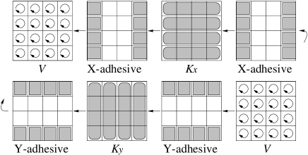
FIG. 2.: The procedure for a two-dimensional periodic system. Here $K_{x}$ and $K_{y}$ show the operations of Cayley’s form, and they operate as if this system is not periodic. X-adhesive and Y-adhesive mean the operations of the exponential of the adhesive operators along the x-axis and the y-axis, respectively. The operation of the adhesive operator needs only the values at the edges of the system.

F Parallelization

The adhesive operator plays another important role. It makes Cayley’s form suitable for parallelization. We use the adhesive operator to represent the second finite difference matrix in the following way:

$$\left[\begin{array}[]{cccc}-2&1&0&0\\ 1&-2&1&0\\ 0&1&-2&1\\ 0&0&1&-2\end{array}\right]\\ =\left[\begin{array}[]{cccc}-2&1&0&0\\ 1&-1&0&0\\ 0&0&-1&1\\ 0&0&1&-2\end{array}\right]+\left[\begin{array}[]{cccc}0&0&0&0\\ 0&-1&1&0\\ 0&1&-1&0\\ 0&0&0&0\end{array}\right]\ .$$ (30)

The interior of the first matrix on the right-hand side is separated into two blocks, which means this system is separated into two physically independent areas. The second matrix, which is the adhesive operator, connects the two areas. A large system is separated into many small areas, and each area is managed by a single processor. Since the exponential of a block diagonal matrix is also a block diagonal matrix, each block is computed by a single processor independently. Data transmission is needed only to compute the adhesive operator. The amount of data transmission is quite small, nearly negligible. The outline of the procedure for a two-dimensional closed system on two processors is schematically described by Fig. 3.

FIG. 3.: The procedure for a two-dimensional closed system on two processors. Adhesive shows the operation of the exponential of the adhesive operator for parallel computing. The operation of the adhesive operator needs only the values at the edges of the areas, so the data transmission between the processors is quite small.

G Adaptive mesh refinement

It is necessary for real space computation to be equipped with an adaptive mesh refinement to reduce the computational cost or to improve the accuracy in some important regions. We improved the adhesive operator to manage a connection of between two regions whose mesh sizes are different, as illustrated in Fig. 4.

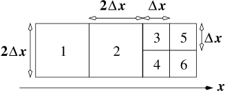
FIG. 4.: An example of adaptive mesh refinement. The element in the left area is twice as large as that in the right area. The adhesive operator connects these areas.

The second differential operator $\partial_{x}^{2}$ should be Hermite, but in this case the condition required for the matrix representation $(\partial_{x}^{2})_{ij}$ is given by

$$(\partial_{x}^{2})_{ij}\Delta{x}_{i}^{2}=(\partial_{x}^{2})_{ji}\Delta{x}_{j}^{2}\ ;\qquad\text{for all {\hbox{i, j}}}.$$ (31)

Considering this condition, an approximation of the second differential operator is given as

$$\partial_{x\rm\hskip 6.02777pt}^{2}=\frac{1}{\Delta{x}^{2}}\begin{tabular*}{159.33542pt}[]{@{\extracolsep{\fill}}|p{8mm}|p{8mm}|p{8mm}|p{8mm}|p{8mm}|p{8mm}|p{8mm}}\cline{1-6}\cr-1/2&1/4&&&&&{1}\\ \cline{1-6}\cr 1/4&-1/2&1/8&1/8&&&{2}\\ \cline{1-6}\cr&1/2&-3/2&&1&&{3}\\ \cline{1-6}\cr&1/2&&-3/2&&1&{4}\\ \cline{1-6}\cr&&1&&-2&&{5}\\ \cline{1-6}\cr&&&1&&-2&{6}\\ \cline{1-6}\cr\end{tabular*}$$ (32)

The indices attached to this matrix indicate the corresponding mesh indices described in Fig. 4. This matrix is also divided into a block-diagonal one and an adhesive operator as

$$\partial_{x\rm bd}^{2}=\frac{1}{\Delta{x}^{2}}\begin{tabular*}{159.33542pt}[]{@{\extracolsep{\fill}}|p{8mm}|p{8mm}|p{8mm}|p{8mm}|p{8mm}|p{8mm}|p{8mm}}\cline{1-6}\cr-1/2&1/4&&&&&{1}\\ \cline{1-6}\cr 1/4&-1/4&&&&&{2}\\ \cline{1-6}\cr&&-1&&1&&{3}\\ \cline{1-6}\cr&&&-1&&1&{4}\\ \cline{1-6}\cr&&1&&-2&&{5}\\ \cline{1-6}\cr&&&1&&-2&{6}\\ \cline{1-6}\cr\end{tabular*}$$ (33)

$$\partial_{x\rm ad}^{2}=\frac{1}{\Delta{x}^{2}}\begin{tabular*}{159.33542pt}[]{@{\extracolsep{\fill}}|p{8mm}|p{8mm}|p{8mm}|p{8mm}|p{8mm}|p{8mm}|p{8mm}}\cline{1-6}\cr&&&&&&{1}\\ \cline{1-6}\cr&-1/4&1/8&1/8&&&{2}\\ \cline{1-6}\cr&1/2&-1/2&&&&{3}\\ \cline{1-6}\cr&1/2&&-1/2&&&{4}\\ \cline{1-6}\cr&&&&&&{5}\\ \cline{1-6}\cr&&&&&&{6}\\ \cline{1-6}\cr\end{tabular*}$$ (34)

The exponential of the adhesive operator is calculated using the following formula:

$$\exp{\left[\frac{{\rm i}\Delta{t}}{4\Delta{x}^{2}}\left(\begin{array}[]{ccc}-1/4&1/8&1/8\\ 1/2&-1/2&0\\ 1/2&0&-1/2\\ \end{array}\right)\right]}=\\ {\bf I}+\left(\begin{array}[]{ccc}2c_{1}&-c_{1}&-c_{1}\\ -4c_{1}&2c_{1}+c_{2}&2c_{1}-c_{2}\\ -4c_{1}&2c_{1}-c_{2}&2c_{1}+c_{2}\end{array}\right)\ ,$$ (35)

where

$$c_{1} \equiv\frac{1}{6}\exp{\Bigl{[}-\frac{3{\rm i}}{\sqrt{2}}\frac{\Delta{t}}{8\Delta{x}^{2}}\Bigr{]}}-\frac{1}{6}\ ,$$ (36)

$$c_{2} \equiv\frac{1}{6}\exp{\Bigl{[}-\frac{2{\rm i}}{\sqrt{2}}\frac{\Delta{t}}{8\Delta{x}^{2}}\Bigr{]}}-\frac{1}{6}\ .$$ (37)

In this way, it is found that the adhesive operator is important to simulate a larger or a more complicated system by the present method.

III Application

In this section, we show some applications of our numerical method. Though these applications treat simple physical systems, they are sufficient for verifying the reliability and efficiency of the method. Throughout this section, we use the atomic units (a.u.).

A Comparison with conventional methods

As far as we know, the conventional methods of solving the TD-Schrödinger equation are classified into three categories: 1) the multistep method[3], 2) the method developed by De Raedt[2] and 3) the method equipped with Cayley’s form[5].

In this section, we make brief comparisons between Cayley’s form and other conventional methods by simply simulating a Gaussian wave packet moving in a one-dimensional free system as illustrated in Fig. 5.

FIG. 5.: The model system for comparison with conventional methods. $256$ computational grid points are allocated in the physical length $8.0\text{a.u.}$ A Gaussian wave packet is placed in the system, whose initial average location $x_{o}$ and momentum $p_{o}$ are set at $x_{o}=2.0\text{a.u.}$ and $p_{o}=12.0\text{a.u.}$, respectively.

The TD-Schrödinger equation of this system is simply given by

$${\rm i}\frac{\partial\psi(x,t)}{\partial t}=-\frac{\partial_{x}^{2}}{2}\ \psi(x,t)\ .$$ (38)

The wavefunction at the initial state is set as a Gaussian:

$$\psi(x,t=0)=\frac{1}{\sqrt[4]{2\pi W^{2}}}\exp{\Bigl{[}-\frac{|x-x_{o}|^{2}}{4W^{2}}+{\rm i}p_{o}x\Bigr{]}}\ ,$$ (39)

where $W=0.25\text{a.u.},\ x_{o}=2.0\text{a.u.},\ p_{o}=12.0\text{a.u.}$

The evolution of this Gaussian is analytically derived as

$$\psi(x,t)=\frac{1}{\sqrt[4]{2\pi W^{2}+(\pi/2)(t/W)^{2}}}\\ \times\exp{\Bigl{[}-\frac{(x-x_{o}-p_{o}t)^{2}}{4W^{2}+(t/W)^{2}}+{\rm i}p_{o}x\Bigr{]}}\ .$$ (40)

Therefore, the average location of the Gaussian $\langle x(t)\rangle$ is derived as if it is a classical particle:

$$\langle x(t)\rangle=\langle x(t=0)\rangle+p_{o}t\ .$$ (41)

This characteristic is useful to check the accuracy of the simulation.

We use the second-order version of the multistep method and the De Raedt’s method in order to compare with Cayley’s form since Cayley’s form is second-order accurate in space and time.

The second-order multistep method we used in this system is given by

$$\psi(t+\Delta{t})=\psi(t-\Delta{t})+{\rm i}2\Delta{t}\frac{\partial_{x}^{2}}{2}\,\psi(t)\ ,$$ (42)

where $\partial_{x}^{2}$ is approximated by a finite difference matrix as

$$\partial_{x}^{2}\simeq\frac{1}{\Delta{x}^{2}}\left[\begin{array}[]{cccccc}-2&1&0&0&0&0\\ 1&-2&1&0&0&0\\ 0&1&-2&1&0&0\\ 0&0&1&-2&1&0\\ 0&0&0&1&-2&1\\ 0&0&0&0&1&-2\end{array}\right]\ .$$ (43)

Extra memories are needed for the wavefunction at the previous time step $\psi(t-\Delta{t})$. Though the time evolution of this method is not unitary, the norm of the wavefunction is conserved with good accuracy on the condition that $\Delta{t}/\Delta{x}^{2}\leq 0.5$. This method needs only $10N$ floating operations per time step, which is the fastest method in conditionally stable methods.

Meanwhile, the second-order De Raedt’s method is given by

$$\psi(t+\Delta{t})=\exp\!\!{\Bigl{[}\frac{{\rm i}\Delta{t}}{2}\frac{\partial_{xa}^{2}}{2}\!\Bigr{]}}\!\exp\!\!{\Bigl{[}{\rm i}\Delta{t}\frac{\partial_{xb}^{2}}{2}\!\Bigr{]}}\!\exp\!\!{\Bigl{[}\frac{{\rm i}\Delta{t}}{2}\frac{\partial_{xa}^{2}}{2}\!\Bigr{]}}\psi(t)$$ (44)

where $\partial_{xa}^{2}$ and $\partial_{xb}^{2}$ are the parts of the second differential operator and are approximated by finite difference matrices as below:

$$\partial_{xa}^{2} \simeq\frac{1}{\Delta{x}^{2}}\left[\begin{array}[]{cccccc}-1&1&0&0&0&0\\ 1&-1&0&0&0&0\\ 0&0&-1&1&0&0\\ 0&0&1&-1&0&0\\ 0&0&0&0&-1&1\\ 0&0&0&0&1&-1\end{array}\right]\ ,$$ (51)

$$\partial_{xb}^{2} \simeq\frac{1}{\Delta{x}^{2}}\left[\begin{array}[]{cccccc}-1&0&0&0&0&0\\ 0&-1&1&0&0&0\\ 0&1&-1&0&0&0\\ 0&0&0&-1&1&0\\ 0&0&0&1&-1&0\\ 0&0&0&0&0&-1\end{array}\right]\ .$$ (58)

The exponentials of those matrices are exactly calculated using the following formula:

$$\exp{\Bigl{[}{\rm i}C\begin{pmatrix}-1&1\\ 1&-1\end{pmatrix}\Bigr{]}}={\bf I}+\frac{1-e^{-2{\rm i}C}}{2}\begin{pmatrix}-1&1\\ 1&-1\end{pmatrix}\ .$$ (59)

The time evolution of this method is exactly unitary, and the norm is exactly conserved unconditionally. However, it seems that the accuracy tends to break down on the condition that $\Delta{t}/\Delta{x}^{2}>1.0$. This method needs $18N$ floating operations per time step, which is the fastest method in unconditionally norm-conserving methods.

Cayley’s form with the finite difference method is given by

$$\psi(t+\Delta{t})=\frac{1+{\rm i}\Delta{t}/4\ \partial_{x}^{2}}{1-{\rm i}\Delta{t}/4\ \partial_{x}^{2}}\,\psi(t)\ ,$$ (60)

where the spatial differential operator is approximated by the ordinary way in Eq. (43).

The time evolution of this method is exactly unitary, and the norm is exactly conserved unconditionally. Moreover, this method maintains good accuracy even under the condition that $\Delta{t}/\Delta{x}^{2}>1.0$. This method needs $26N$ floating operations per time step, which is the fastest method in unconditionally stable methods.

We have simulated the motion of the Gaussian by those methods. First we show a comparison of Cayley’s form with the conventional methods in the framework of the FDM. Figure 6 shows the time evolution of the error in the energy, which is evaluated by the finite difference method as described below

$$\epsilon(t)=E(t)-E(t=0)$$ (61)

$$E(t)=-\frac{1}{2\Delta{x}}{\rm Re}\sum_{i=0}^{N-1}\psi_{i}^{\ast}(t)\bigl{(}\psi_{i-1}(t)-2\psi_{i}(t)+\psi_{i+1}(t)\bigr{)}\ .$$ (62)

The initial energy is evaluated as $73.03\text{a.u.}$, though it is theoretically expected to be $74\text{a.u.}$ The ratio $\Delta{t}/\Delta{x}^{2}$ is set at $0.5$ to meet the stable condition required for the multistep method.

The energies violently oscillate in the results of the multistep method and De Raedt’s method, as a result of the fact that these time evolution operators do not commute with the Hamiltonian. These energies seem to converge after the wave packet is delocalized in a uniform way over the system. Meanwhile, the energy is conserved exactly in the result of Cayley’s form because Cayley’s form commutes with the spatial second differential operator which is the Hamiltonian itself in this system.

Figure 7 shows the relation of the time slice $\Delta{t}$ to the error in the average momentum of the Gaussian, which is evaluated by the finite difference method as described below:

$$\epsilon(\Delta{t}/\Delta{x}^{2})=\frac{\langle x(t=T)\rangle-\langle x(t=0)\rangle}{T}-\langle p(t=0)\rangle\ ,$$ (63)

$$\langle x(t)\rangle=\Delta{x}\sum_{i=0}^{N-1}x_{i}|\psi_{i}(t)|^{2}$$ (64)

$$\langle p(t)\rangle=\frac{1}{2}{\rm Im}\sum_{i=0}^{N-1}\psi_{i}(t)^{\ast}\bigl{(}\psi_{i+1}(t)-\psi_{i-1}(t)\bigr{)}\ ,$$ (65)

where $T$ is a time span set at $0.4\text{a.u.}$ The initial momentum $\langle p(t=0)\rangle$ is calculated as $11.7\text{a.u.}$, which is different from the theoretical value $p_{o}=12.0\text{a.u.}$ due to the finite difference method.

FIG. 6.: Time variances in the energies computed by the three methods. The time slice is set at $\Delta{t}=1/2048\text{a.u.}$ and the spatial slice is set at $\Delta{x}=1/32\text{a.u.}$ so that the ratio $\Delta{t}/\Delta{x}^{2}$ is equal to $0.5$. The energies violently oscillates in the result of the multistep method and De Raedt’s method. Meanwhile, the energy is conserved exactly in the result of Cayley’s form.

FIG. 7.: Errors in the average momentum computed by the three methods in several time slices. The multistep method cannot be performed when $\Delta{t}/\Delta{x}^{2}>0.5$. The error of De Raedt’s method is too large when $\Delta{t}/\Delta{x}^{2}>1$. The error of Cayley’s form is rather small. The spatial slice is set at $\Delta{x}=1/32\text{a.u.}$

In the multistep method, the computation cannot be performed due to a floating exception, if the ratio $\Delta{t}/\Delta{x}^{2}$ exceeds $0.5$. In De Raedt’s method, the error becomes too large to plot in this graph if the ratio $\Delta{t}/\Delta{x}^{2}$ exceeds $1.0$. Meanwhile, in Cayley’s form, the error is not so large even if the ratio $\Delta{t}/\Delta{x}^{2}$ exceeds $1.0$.

In this way, Cayley’s form is found rather stable. Therefore, we can use a longer time slice than those of the other methods. And this Cayley’s form becomes suitable for three-dimensional systems, potentials, periodic conditions, adaptive mesh refinement, and parallelizations by our improvements in this paper.

B Test of the adhesive operator

To verify the reliability and efficiency of the adhesive operator for periodic condition and parallelization, we have simulated the motion of a Gaussian wave packet in a two-dimensional free system. As illustrated in Fig. 8, this system has periodic conditions along both the x-axis and the y-axis, and it is divided into nine areas, each of them is managed by a single processing element; the adhesive operator connects them. The initial wavefunction is set as a Gaussian given as

$$\psi({\bf r},t=0)=\frac{1}{\sqrt{2\pi W^{2}}}\exp{\Bigl{[}-\frac{|{\bf r}-{\bf r_{o}}|^{2}}{4W^{2}}+{\rm i}{\bf p_{o}}\cdot{\bf r}\Bigr{]}}\ ,$$ (66)

where ${\bf r_{o}}$ is set as the center of this system and ${\bf p_{o}}=(1\text{a.u.},1\text{a.u.})$, $W=1\text{a.u.}$ The energy of this Gaussian is theoretically derived as $1.0625\text{a.u.}$

FIG. 8.: The model system for the test of the adhesive operator for periodic conditions and parallelization. This system is periodically connected and is divided into nine areas. Each area is managed by a single processing element. $32\times 32$ computational grid points are allocated in each area whose physical size is set at $8.0\text{a.u.}\times 8.0\text{a.u.}$ The time slice is set at $\Delta{t}=1/16\text{a.u.}$

Figure 9 shows snapshots of the time evolution of the Gaussian, which is observed to go through these areas smoothly. Figure 10 shows the evolution of the energy, which is observed to oscillate around its initial value.

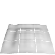
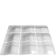
FIG. 9.: Evolution of the density. The Gaussian is observed to go through these areas smoothly.

FIG. 10.: Time variance in the energy. The initial energy is theoretically derived as $1.0625\text{a.u.}$, but it is evaluated as $1.0553\text{a.u.}$ by the FDM. The energy oscillates near its initial value but never drifts monotonously.

Second, we allocate $64\times 64$ grid points only in the central area as illustrated in Fig. 11. We utilize the adhesive operator for the adaptive mesh refinement. Figure 12 shows the snapshots, with the Gaussian going through these areas smoothly. Figure 13 shows the evolution of the energy, which is observed to oscillate near its initial value. In this way, the reliability of the adhesive operator is proved.

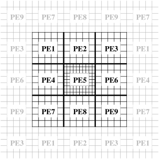
FIG. 11.: The model system for the test of the adhesive operator for the adaptive mesh refinement. This system is also periodically connected and is divided into nine areas. Each area is managed by a single processing element. The size of each area is set at $8.0\text{a.u.}\times 8.0\text{a.u.}$  $32\times 32$ computational grid points are allocated in each areas except the central area. The central area has $64\times 64$ computational grid points, which makes it twice as fine as those of the other areas. The time slice is set at $\Delta{t}=1/16\text{a.u.}$

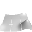
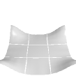
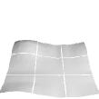
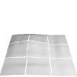
FIG. 12.: Evolution of the density. The Gaussian is observed to go through these areas smoothly.

FIG. 13.: Time variance in the energy. The initial energy is theoretically derived as $1.0625\text{a.u.}$, but it is evaluated as $1.0591\text{a.u.}$ by the FDM. The energy oscillates near its initial value but it never drifts monotonously.

C Excitation of a hydrogen

As the last application of the present method, we demonstrate its validity and efficiency in describing the process of photon-induced electron excitation in a hydrogen atom in a strong laser field. The laser is treated as a classically oscillating electric force polarized in the z-direction:

$$E_{z}=E_{o}\sin{\omega t}\ .$$ (67)

The spatial variation of the electric field of the light is neglected, because the electron system is much smaller than the order of the wave length. Then the interaction term of the Hamiltonian is approximated as

$${\cal H}_{\rm int}=-eE_{z}z\ .$$ (68)

In other words, we only take into account the electro-dipole interaction of the electron with the light, and neglect the electro-quadrapole, the magnetic-dipole, and other higher interactions.

The amplitude $E_{o}$ is set at $1/64\text{a.u.}=0.80\text{V/\AA}$, which is as strong as a usual pulse laser. The angular frequency $\omega$ is set at $0.3125\text{a.u.}=8.5\text{eV}$, less than the transition energy between 1S and 2P. Ordinarily, such low energetic electric force has no effect on the electronic excitation. But with such a strong amplitude, various nonlinear optical effects are caused by the electron dynamics.

We allocate $128^{3}$ grid points in a $32^{3}\text{a.u.}^{3}$ cubic closed system. The hydrogen nucleus is located at the center of the system, and the nucleus potential is constructed by solving the Poisson equation in the discretized space to avoid the singularity of the nucleus potential. The 1S-orbital is assumed as the initial state of the wavefunction. Then we turn on the electric field and start the simulation. The time slice is set at $0.0785\text{a.u.}=2.0\times 10^{-3}\text{fs}$ so as to follow the rapid variation of the wavefunction and the electric force. We follow the evolution for $32\text{k}$ iteration.

Figure 14 shows the time variance in the polarization of the electron. The oscillation of the polarization generates another electric field, which corresponds to a non-linearly scattered light from the atom. By Fourier-transforming the polarization along the time axis, we obtained the spectrum of the scattered light shown in Fig. 15.

FIG. 14.: Time variance in the polarization of the electron.

FIG. 15.: Spectrum of the scattered light generated by the oscillation of the electron.

Several sharp peaks are found, which are interpreted as follows: The peak at $8.5\text{eV}$ comes from Rayleigh scattering, whose frequency is identical with the injected light: $\omega$. The peak at $10.2\text{eV}$ comes from Lyman $\alpha$ emission, which is generated by the electron transition from the 2P-orbital to the 1S-orbital: $\omega_{L_{\alpha}}$. On the other hand, the peak at $12.1\text{eV}$ comes from Lyman $\beta$ emission, which is generated by the electron transition from the 3P-orbital to the 1S-orbital: $\omega_{L_{\beta}}$. The peak at $6.8\text{eV}$ comes from hyper Raman scattering, whose frequency is identical with $2\omega-\omega_{L_{\alpha}}$. Moreover the peak at $25.5\text{eV}$ comes from the third harmonic generation, whose frequency is identical with $3\omega$.

The simulation is also performed for a different laser frequency; the injecting photon energy $\omega$ is set at $10.2\text{eV}$, which is the same as the transition energy between 1S and 2P. In this case the electron starting from a 1S orbital is expected to excite to a 2Pz orbital. Figure 16 shows the snapshots of the density during the simulation time span.

FIG. 16.: Evolution of the density of the electron in the hydrogen atom. The density starting from a 1S orbital oscillates with time and becomes a 2Pz orbital.

Figure 17 and Fig. 18 show the polarization and the spectrum, respectively. Three peaks are found, at $9.9\text{eV}$, $10.2\text{eV}$, and $10.5\text{eV}$. These peaks are derived from the theory of the Dressed atom or the AC stark effect as below:

$$\omega-eE_{o}\left<{\rm 2P_{z}}|z|{\rm 1S}\right>,\ \omega,\ \omega+eE_{o}\left<{\rm 2P_{z}}|z|{\rm 1S}\right>\ .$$ (69)

FIG. 17.: Time variance in the polarization of the electron.

FIG. 18.: Spectrum of the scattered light generated by the oscillation of the electron.

One could obtain such behavior analytically by using perturbation theory; however, with the present method, we could directly calculate them without perturbation theory and without information on the excited states of the system.

IV Conclusion

We have formulated a new method for solving the time-dependent Schrödinger equation numerically in real space. We have found that by using Cayley’s form and Suzuki’s fractal decomposition, the simulation can be fast, stable, accurate, and suitable for vector-type supercomputers. We have proposed the adhesive operator to make Cayley’s form suitable for periodic systems and parallelization and adaptive mesh refinement.

These techniques will also be useful for the time-dependent Kohn Sham equation, which is our future work.

V Acknowledgments

We are indebted to Takahiro Kuga for his suggestions concerning non-linear optics. Calculations were done using the SR8000 supercomputer system at the Computer Centre, University of Tokyo.

REFERENCES

• [1] R. Varga, Matrix Iterative Analysis (Prentice-Hall, Englewood Cliffs, NJ, 1962), p.273.
• [2] H. De Raedt and K. Michielsen, Computers in Physics, 8, 600 (1994).
• [3] T. Iitaka, Phys. Rev. E 49, 4684 (1994).
• [4] H. Natori and T Munehisa, J. Phys. Soc. Japan 66, 351 (1997).
• [5] Numerical Recipes in C, chapter 19, section 2, W. H. Press, S. A. Teukolsky, W. T. Vetterling and B. P. Flannery, (Cambridge University Press, 1996).
• [6] H. De Raedt and K. Michielsen, Phys. Rev. B. 50, 631 (1994)
• [7] T. Iitaka, S. Nomura, H. Hirayama, X. Zhao, Y. Aoyagi and T. Sugano, Phys. Rev. E 56, 1222 (1997).
• [8] H. Kono, A. Kita, Y. Ohtsuki and Y. Fujimura, J. Comput. Phys. (USA), 130, 148 (1997).
• [9] M. Suzuki, Phys. Lett. A 146, 319 (1990).
• [10] M. Suzuki, J. Math. Phys. 32, 400 (1991).
• [11] K. Umeno and M. Suzuki, Phys. Lett. A 181, 387 (1993).
• [12] M. Suzuki, Proc. Japan Acad. 69 Ser. B, 161 (1993).
• [13] M. Suzuki and K. Umeno, Vol. 76 of Springer Proceedings in Physics, (Computer Simulation Studies in Condensed-Matter Physics VI, editied by D. P. Landau, K. K. Mon, H. B. Schüttler, Springer, Berlin, 1993), p. 74.
• [14] M. Suzuki, Phys. Lett. A 201, 425 (1995).