A Method to Extract Potentials from the Temperature Dependence of Langmuir Constants for Clathrate-Hydrates

Abstract

It is shown that the temperature dependence of Langmuir constants contains all the information needed to determine spherically averaged intermolecular potentials. An analytical “inversion” method based on the standard statistical model of van der Waals and Platteeuw is presented which extracts cell potentials directly from experimental data. The method is applied to ethane and cyclopropane clathrate-hydrates, and the resulting potentials are much simpler and more meaningful than those obtained by the usual method of numerical fitting with Kihara potentials.

1 Introduction

A central mission of chemical physics is to determine intermolecular interactions from experimental phase equilibrium data. This is generally a very difficult task because macroscopic equilibrium constants reflect averaging over vast numbers of poorly understood microscopic degrees of freedom. Since the advent of the computer, empirically guided numerical fitting has become the standard method to obtain intermolecular potentials. An appealing and often overlooked alternative, however, is to solve inverse problems based on simple statistical mechanical models.

A well-known class of inverse problems is to determine the density of states $n(E)$ from the partition function $Q(\beta)$, or one of its derivatives, as a function of inverse temperature $\beta=1/kT$. For classical Maxwell-Boltzmann statistics, these quantities are simply related by an Laplace transform [1]

$$Q(\beta)=\int_{0}^{\infty}e^{-\beta\varepsilon}n(\varepsilon)d\varepsilon$$ (1)

which is straightforward to invert. Analogous quantum-mechanical problems have also been solved using Laplace (or Mellin) transform methods. For example, in Bose-Einstein statistics,

$$Q(\beta)=\int_{0}^{\infty}\frac{n(\varepsilon)d\varepsilon}{e^{\beta\varepsilon}+1},$$ (2)

the phonon density of states can be obtained from the specific heat of a crystal [2, 3, 4, 5, 6, 7, 8, 9], and the area distribution of a blackbody radiator can be obtained from its power spectrum [10, 11, 12, 5, 6]. Similarly, in Fermi-Dirac statistics,

$$Q(\beta)=\int_{0}^{\infty}\frac{n(\varepsilon)d\varepsilon}{e^{\beta(\varepsilon-\varepsilon_{F})}-1},$$ (3)

the band structure of a doped semiconductor can be obtained from the temperature dependence of its carrier density [13]. In each of these examples, it is possible to extract the microscopic density of states from a temperature-dependent thermodynamic quantity because each is a function of just one variable.

In the more complicated case of chemical systems, thermodynamic quantities are related to classical configurational integrals,

$$Z(\beta)=\int_{V}e^{-\beta\Phi(\vec{r})}d\vec{r},$$ (4)

where the total energy $\varepsilon$ in Eq. (1) is replaced by the intermolecular potential $\Phi(\vec{r})$ , and the integral extends over the interaction volume $V$. Unfortunately, these integrals are multi-dimensional, which leads to under-determined inverse problems. Perhaps as a result, statistical inversion methods have apparently not been developed for intermolecular potentials in chemical systems, and instead empirical fitting has been used exclusively to describe phase equilibrium data.

In this article, we show that within the common spherical-cell approximation the intermolecular potential is completely determined by the temperature dependence of the Langmuir constant. In this case, the linear integral equation (1) is replaced by a non-linear equation of the form

$$Z(\beta)=4\pi\int_{0}^{\infty}e^{-\beta w(r)}r^{2}dr$$ (5)

where $w(r)$ is a spherically averaged “cell potential” [24]. As shown below in the important case of Langmuir constants for clathrate-hydrates, this simple inverse problem can be solved exactly without resorting to numerical fitting schemes.

Before proceeding, we mention some related ideas in the recent literature of solid state physics. As with chemical systems, empirical fitting is also the standard approach to derive interatomic potentials for metals and semiconductors. Since the pioneering work of Carlsson, Gelatt, and Ehrenreich in 1980 [14, 15], however, exact inversion methods have been developed to obtain potentials from cohesive energy curves [5, 16, 17, 18, 19, 20]. These theoretical advances, discussed briefly in Appendix A, have recently led to improvements in the modeling of silicon, beyond what had previously been obtained by empirical fitting alone [20, 21]. Inspired by such developments in solid state physics, here we seek similar insights into clathrate-hydrate intermolecular forces, albeit using a very different statistical mechanical formalism.

2 The Inverse Problem for Clathrate-Hydrates

2.1 The Statistical Theory of van der Waals and Platteeuw

Clathrate-hydrates exist throughout nature and are potentially very useful technological materials [22]. For example, existing methane hydrates are believed to hold much more energy than any fossil fuel in use today. Carbon dioxide hydrates are being considered as effective materials for the sequestration and/or storage of CO₂. In spite of their great importance, however, the theory of clathrate-hydrate phase behavior is not very well developed, still relying for the most part on the ad hoc empirical fitting of experimental data. Therefore, we have chosen to develop our statistical inversion method in the specific context of clathrate-hydrate chemistry.

Since being introduced in 1959, the statistical thermodynamical model of van der Waals and Platteeuw (vdWP) has been used almost exclusively to model the phase behavior of clathrate-hydrates, usually together with a spherical cell (SC) model for the interaction potential between the enclathrated or “guest” molecule and the cage of the clathrate-hydrate. The SC model was also introduced by vdWP, inspired by an analogous approximation made by Lennard-Jones and Devonshire in the case of liquids [23, 24].

In the general formulation of vdWP [23], the chemical potential difference between an empty, unstable hydrate structure with no guest molecules, labeled MT, and the stable hydrate, labeled H, is related to the so-called Langmuir hydrate constant $C_{Ji}$ and the fugacity of the guest molecule $\hat{f}_{J}$

$$\Delta\mu^{MT-H}=kT\sum_{i}\nu_{i}\ln(1+\sum_{J}C_{Ji}\hat{f}_{J})$$ (6)

where $i$ designates the type of cage, $\nu_{i}$ the number of cages of type $i$ per water molecule and $J$ the type of guest molecule. In practice, experimental phase equilibria data is used to determine $\Delta\mu^{MT-H}$.

The connection with intermolecular forces within vdWP theory is made by expressing the Langmuir hydrate constant as the configurational integral $Z_{Ji}$ divided by $kT$, which is written explicitly as an integral over the volume $V$

$$C_{Ji}(T)=\frac{1}{8\pi^{2}kT}\int_{V}e^{-\Phi(r,\theta,\phi,\alpha,\xi,\gamma)/kT}r^{2}sin\theta sin\xi drd\theta d\phi d\alpha d\xi d\gamma$$ (7)

where $\Phi(r,\theta,\phi,\alpha,\xi,\gamma)$ is the general six dimensional form of the interaction potential between the guest molecule at spherical coordinates $(r,\theta,\phi)$ oriented with Euler angles $(\alpha,\xi,\gamma)$ with respect to all of the water molecules in the clathrate-hydrate.

In the SC approximation, which is made without any careful mathematical justification, the intermolecular potential $\Phi$ is replaced by a spherically averaged cell potential $w(r)$, which reduces the Langmuir constant formula (7) to a single, radial integration

$$C_{Ji}(T)=\frac{4\pi}{kT}\int_{0}^{R}e^{-w(r)/kT}r^{2}dr$$ (8)

where the cutoff distance $R$ is often arbitrarily taken as the radius of the cage. (As shown below, the exact value rarely matters because temperatures are typically so low that the high energy portion of the cage $r\approx R$ makes a negligible contribution to the integral.) Although the SC approximation may appear to be a drastic simplification, it is nevertheless very useful for theoretical studies of intermolecular forces based on Langmuir constant measurements.

2.2 Numerical Fitting Schemes

Before this work, the functional form of the cell potential $w(r)$ has always been obtained by first choosing a model interaction potential between the guest molecule in a cage and each nearest neighbor water molecule essentially ad hoc, and then performing the spherical average from (7) to (8) analytically. The most common potential form in use today is the Kihara potential, which is simply a shifted Lennard-Jones potential with a hard-core. Using the Kihara potential and spherically averaging the interaction energy, typically over the first-shell only, yields the following functional form for $w(r)$:

$$w(r)=2z\epsilon[\frac{\sigma^{12}}{R^{11}r}(\delta_{10}+\frac{a}{R}\delta_{11})-\frac{\sigma^{6}}{R^{5}r}(\delta_{4}+\frac{a}{R}\delta_{5})]$$ (9)

where

$$\delta_{N}=\frac{1}{N}[(1-\frac{r}{R}-\frac{a}{R})^{-N}-(1+\frac{r}{R}-\frac{a}{R})^{-N}]$$ (10)

and $z$ is the coordination number, $R$ is the radius of the cage, and $\sigma$, $\epsilon$, and $a$ are the Kihara parameters. As a result of the averaging process leading from (7) to (8), the functional form of $w(r)$ is fairly complicated, and the parameters $\epsilon$ and $\sigma$ are generally determined by fitting monovarient equilibrium temperature-pressure data numerically [22, 25].

There are several serious drawbacks to this ubiquitous numerical fitting procedure, which suggest that the Kihara parameters lack any physical significance: $(i)$ The Kihara parameters are not unique, and many different sets can fit the experimental data well; $(ii)$ the Kihara parameters found by fitting Langmuir curves do not match those of found by fitting other experimental data, such as the second virial coefficient or the gas viscosity [22]; and $(iii)$ comparisons of Langmuir constants found via the SC approximation (8) and via explicit multi-dimensional quadrature (7) show that the two can differ by over 12 orders of magnitude [26, 27] (which results from the exponentially strong sensitivity of the Langmuir constant to changes in the cell potential). These problems call into question the validity of using the Kihara potential as the basis for the empirical fitting, and even the use of the SC approximation itself.

2.3 Inversion of Langmuir Curves

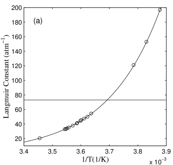
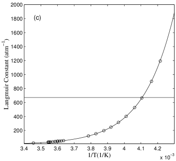
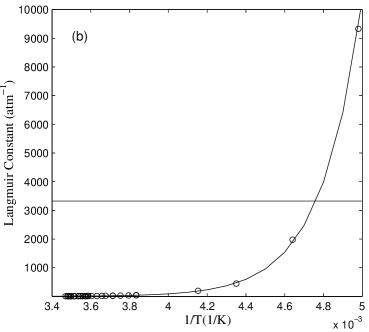
Figure 1: Exponential fits of Langmuir constants over the measured temperature range plotted with linear axes for (a)-(b) cyclopropane and (c) ethane clathrate-hydrates. An enlargement of the high temperature data for cyclopropane is shown in (a). The experimental data is taken from Ref. [28].

It would clearly be preferable to extract more reliable information about the interatomic forces in clathrate-hydrates directly from experimental data without any ad hoc assumptions about their functional form. In principle, such an approach is possible for clathrate-hydrates which contain a single type of guest molecule occupying only one type of cage. In this case, each of the sums in Eq. (6) contains only one term, and by using an equation of state to compute the fugacity $\hat{f}_{J}$, the Langmuir constant $C_{Ji}$ can be determined directly from experimental phase equilibria data. Typical data sets obtained in this manner are shown in Fig. 1 for Structure I ethane and cyclopropane clathrate-hydrates [28].

Because the full potential $\Phi$ in (7) is multi-dimensional (while the Langmuir constant only depends on a single parameter $T$), the general vdWP theory is too complex to pose a well-defined inverse problem for the interatomic forces. The SC approximation, on the other hand, introduces a very convenient theoretical construct, the spherically averaged potential $w(r)$, which has the same dimensionality as the Langmuir curve $C_{Ji}(T)$ of a single type of guest molecule occupying a single type of cage. (Since we consider only this case, we drop the subscripts $Ji$ hereafter.) Although one can question the accuracy of the SC approximation, its simplicity at least allows precise connections to be made between the Langmuir curve and the cell potential.

As an appealing alternative to empirical fitting, in this article we view Eq. (8) as an integral equation to be solved analytically for $w(r)$, given a particular Langmuir curve $C(T)$. Letting $\beta=1/kT$, we rewrite (8) as

$$C(\beta)=4\pi\beta\int_{0}^{\infty}e^{-\beta w(r)}r^{2}dr,$$ (11)

where we have also set the upper limit of integration to $R=\infty$, which introduces negligible errors due to the very low temperatures (large $\beta$) accessible in experiments. (This will be justified a posteriori with a precise definition of “low” temperatures below.) Note that Eq. (11) has the form of Eq. (5) with $Z(\beta)=\beta C(\beta)$.

2.4 Application to Experimental Data

In our analytical approach, some straight-forward fitting of the raw experimental data is needed to construct the function $C(\beta)$, but after that, the “inversion” process leading to $w(r)$ is exact. For example, typical sets of experimental data are well described by a van’t Hoff temperature dependence

$$C(\beta)=C_{o}e^{m\beta}$$ (12)

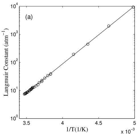
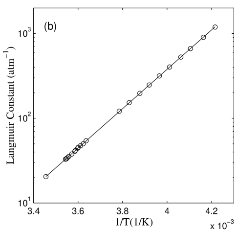
Figure 2: Exponential dependence with inverse temperature of experimental Langmuir curves from Fig. 1 plotted with log-linear axes for (a) ethane and (b) cyclopropane clathrate hydrates. Straight lines indicate pure van’t Hoff behavior.

as shown in Fig. 2 for ethane and cyclopropane clathrate hydrates [28], and the constant $m$ is generally positive. (Note that the exponential dependence which we call ”van’t Hoff dependence” in this paper can be expected based on quite general thermodynamic considerations [29].)

Aided by the analysis, the quality and functional form of these fits are discussed below in section 7. In order to allow for deviations from the dominant van’t Hoff behavior, however, in this article we consider the more general form

$$C(\beta)=\beta F(\beta)e^{m\beta}$$ (13)

where $m$ is a constant defined by

$$m=\lim_{\beta\rightarrow\infty}\log C(\beta)/\beta$$ (14)

whenever this limit exists and is finite, i.e. when the prefactor $F(\beta)$ in Eq. (13) is dominated by the exponential term at low temperatures. We exclude the possibility of hyper-exponential behavior at low temperatures, $\log C/\beta\rightarrow\infty$, which is not physically meaningful, as explained below. The set of possible prefactors includes power-laws, $F(\beta)=\beta^{-\mu}$, as well as various rational functions.

The rest of article is organized as follows. In section 3 we discuss various necessary and sufficient conditions for the existence of physically reasonable solutions, and we also derive the asymptotics of the Langmuir curve at low temperature from the behavior of the cell potential at near its minimum. In section 4, we perform the analysis in the general case, and in section 5, we discuss the specific case of van’t Hoff dependence (12), which leads to a cubic solution as well as various unphysical solutions involving cusps. In section 6, we derive analytical solutions for several different temperature dependences, which reveal the significance of possible deviations from van’t Hoff behavior for the form of the potential $w(r)$. The theoretical curves are compared with the experimental data in section 7, and the physical conclusions of the analysis are summarized in section 8. Relevant mathematical theorems are proved in the Appendix B.

3 General Analysis of the Inverse Problem

3.1 Necessary Conditions for the Existence of Solutions

On physical grounds, it expected that the cell potential $w(r)$ is continuous (at least piecewise) and has a finite minimum at $r_{o}\geq 0$ somewhere inside the clathrate cage, $w(r)\geq w(r_{o})=w_{o}$. We also allow the possibility that $w(r)$ is infinite for certain values of $r$ (e.g. outside a “hard-wall radius”) by simply omitted such values from the integration in Eq. (11). As proved in the Appendix B, these simple physical requirements suffice to imply the asymptotic relation (14), where $m=-w_{o}$. They also place important constraints on the prefactor $F(\beta)$ defined in (13), which must be

• analytic in the half plane $\mbox{Re}\beta>c$ and

• real, positive and non-increasing for $\beta>c$ on the real axis

where $c\geq 0$ is a real number. (Note that we view the inverse temperature $\beta$ as a complex variable, for reasons soon to become clear.) Moreover, if the set

$$S=\{r\geq 0|w_{o}<w(r)<\infty\}$$ (15)

has nonzero measure, then $F(\beta)$ is strictly decreasing on the positive real axis. It is straightforward to generalize these rigorous results to the multi-dimensional integral of vdWP theory, Eq. (7), without making the spherical cell approximation, as described in the Appendix B, but hereafter we discuss only the spherically averaged integral equation, Eq. (11), because it makes possible an exact inversion.

In this section, we give simple arguments to explain the results proved in Theorem 1 of the Appendix B. First, we consider the illustrative example of a constant cell potential with a hard wall at $r=r_{hw}>0$,

$$w(r)=\left\{\begin{array}[]{ll}w_{o}&\mbox{ if }0\leq r<r_{hw}\\ \infty&\mbox{ if }r>r_{hw}\end{array}\right.$$ (16)

which satisfies the assumptions stated above. The integral (11) is easily performed in this case to yield

$$C(\beta)=\frac{4}{3}\pi r_{hw}^{3}\beta e^{-w_{o}\beta}$$ (17)

which implies $m=-w_{o}$, the well depth, and $F(\beta)=\frac{4}{3}\pi r_{hw}^{3}$, the volume of negative energy. Consistent with the general results above, $F(\beta)$ is constant in this case since $S=\emptyset$. For continuous potentials $w(r)$, however, the prefactor $F(\beta)$ must be strictly decreasing because $S\neq\emptyset$.

The integral equation (11) can be simplified by a change of variables from radius to volume. In terms of a shifted cell potential versus volume

$$u(x)=w(r)-w_{o}\ \ \mbox{ where }\ \ x=\frac{4\pi}{3}r^{3}$$ (18)

the integral equation is reduced to the form

$$C(\beta)=\beta F(\beta)e^{-w(r_{o})\beta}$$ (19)

where

$$F(\beta)=\int_{0}^{\infty}e^{-\beta u(x)}dx.$$ (20)

Since $u(x)\geq 0$ by construction, the function $F(\beta)$ is clearly non-increasing. In the Appendix B, it is proved that if the potential varies continuously near its minimum (in a very general sense), then $F(\beta)$ does not decay exponentially. Since $F(\beta)$ also positive and bounded above, we conclude

$$\lim_{\beta\rightarrow\infty}\log C(\beta)/\beta=-w_{o}$$ (21)

which implies $m=-w_{o}$. Therefore, the slope of the Langmuir curve on a “van’t Hoff plot” ($\log C$ versus $\beta=1/kT$) in the low temperature limit is equal to (minus) the minimum energy of the cell potential. Since it is generally observed that $m$ is positive, as in the case of ethane and cyclopropane clathrate-hydrates shown in Figs. 1–2, the cell potential must be attractive, $w_{o}=-m<0$, which simply indicates that the total internal energy is lowered by the introduction of guest molecules into clathrate-hydrates.

The fact that $F(\beta)$ must be nondecreasing has important consequences for the existence of solutions which are piecewise continuous and bounded below. For example, consider the class of Langmuir curves of the form

$$C(\beta)=\beta^{\nu}e^{m\beta}$$ (22)

which is useful in fitting experimental data (see below). We have already addressed the borderline case, $\nu=1$, in which a discontinuous hard-wall solution is possible. Although it is not obvious a priori, there are no solutions to the inverse problem if $\nu>1$, since in that case $F(\beta)=\beta^{\nu-1}$ is increasing. On the other hand, if $\nu<1$, then well-behaved continuous solutions are possible, because $F(\beta)$ is strictly decreasing.

3.2 Low Temperature Asymptotics of the Langmuir Curve

¿From Eq. (21), we see that the minimum energy $w_{o}=w(r_{o})$ determines the leading order asymptotics of $C(\beta)$ in the low temperature limit. More generally, one would expect that $C(\beta)$ at low temperatures is completely determined by shape of the cell potential at low energies, close to its minimum. Using standard methods for the asymptotic expansion of Laplace integrals [30], it is straightforward to provide a mathematical basis for this intuition. For simplicity, here we consider the usual case of a parabolic minimum

$$w(r)=w_{o}+\frac{1}{2}k(r-r_{o})^{2}+O((r-r_{o})^{3})$$ (23)

for some constants $k>0$ and $r_{o}\geq 0$, although below we will derive many exact solutions with non-parabolic minima.

Due to the factor of $r^{2}$ appearing in the integrand in Eq. (11), the two cases of a non-central or central minimum, $r_{o}>0$ and $r_{o}=0$, respectively, must be treated separately. Physically, this qualitative difference between central and non-central-wells is due to the spherical averaging process going from Eq. (7) to Eq. (11): A central well in $w(r)$ corresponds to a unique local minimum of the multidimensional potential $\Phi$, but a non-central-well in $w(r)$ corresponds to a nonlocal minimum of $\Phi$ which is smeared across a sphere of radius $r_{o}$.

Beginning with non-central-well case, $r>0$, we have the following asymptotics as $\mbox{Re}\beta\rightarrow\infty$:

$$C(\beta) \sim 4\pi r_{o}^{2}\beta\int_{r_{o}-\epsilon}^{r_{o}+\epsilon}e^{-\beta(w_{o}+\frac{1}{2}k(r-r_{o})^{2})}dr$$ (24)

$$\sim 4\pi r_{o}^{2}\left(\frac{2\beta}{k}\right)^{1/2}e^{-\beta w_{o}}\int_{-\infty}^{\infty}e^{-t^{2}}dt$$

$$= 4\pi r_{o}^{2}\left(\frac{2\pi\beta}{k}\right)^{1/2}e^{-\beta w_{o}}$$

which is the usual leading order term in the expansion of a Laplace integral [30]. Therefore, the experimental signature of a non-central-well is a Langmuir constant which behaves at low temperatures like

$$C(\beta)\sim C_{o}e^{m\beta}\beta^{1/2}\mbox{ as }\beta\rightarrow\infty.$$ (25)

Comparing (24) and (25), we can identify the well depth $w_{o}=-m$, consistent with the general arguments above, but it is impossible to determine independently the location of $r_{o}$ and the curvature $k$ of the minimum. Instead, any $r_{o}$ and $k$ satisfying $4\pi r_{o}^{2}\sqrt{2\pi/k}=C_{o}$ would exactly reproduce the same large-$\beta$ asymptotics of the Langmuir curve (as would a completely different central-well solution described in section 6). This degeneracy of non-central-well solutions revealed in the low temperature asymptotics is actually characteristic of all non-central-well solutions, as explained below.

In the central-well case, $r_{o}=0$, the asymptotics must be carried out more carefully because the leading term derived in (24) vanishes:

$$C(\beta) \sim 4\pi\beta\int_{0}^{\epsilon}e^{-\beta(w_{o}+\frac{1}{2}kr^{2})}r^{2}dr$$ (26)

$$\sim 4\pi\left(\frac{2}{k^{3}\beta}\right)^{1/2}e^{-\beta w_{o}}\int_{0}^{\infty}t^{1/2}e^{-t}dt$$

$$= \left(\frac{2\pi}{k}\right)^{3/2}\frac{e^{-\beta w_{o}}}{\beta^{1/2}}.$$

The experimental signature of a parabolic central well in the Langmuir curve,

$$C(\beta)\sim C_{o}e^{m\beta}\beta^{-1/2}\mbox{ as }\beta\rightarrow\infty,$$ (27)

is qualitatively different from (25), which provides an unambiguous way to separate the two cases using low temperature measurements. Moreover, unlike the non-central-well case, the curvature $k=2\pi C_{o}^{-2/3}$ of a parabolic central minimum is uniquely determined by the low temperature asymptotics of the Langmuir curve. Consistent with asymptotic results, we shall see in section 4 that central-well solutions to the inverse problem are unique, while non-central-well solutions are not.

3.3 Sufficient Conditions for the Existence of Solutions

The primary difficulty in solving Eq. (11) lies in its being a nonlinear integral equation of the “first kind” for which no general theory of the existence and uniqueness of solutions exists [31, 32]. In the linear case, however, there is a special class of first-kind equations which can be solved using Laplace, Fourier or Mellin transforms, namely integral equations of the additive or multiplicative convolution type [34, 35]

$$\Psi(x) = \int_{-\infty}^{\infty}K(x-y)\psi(y)dy$$ (28)

$$\mbox{ or \ \ \ }\Psi(x) = \int_{0}^{\infty}K(xy)\psi(y)dy,$$ (29)

respectively, where $\psi(x)$ is the unknown function and $\Psi(x)$ is given. Integral equations of the multiplicative form (29) often arise in statistical mechanics as explained in the Introduction.

Although our nonlinear, first-kind equation (11) is not of the convolution type because the unknown function $w(r)$ appears in the exponent, it does somewhat resemble a Laplace transform. This connection is more obvious in the alternative formulation (20) relating $F(\beta)$ and $u(x)$, which is equivalent to the original equation (11) according to the analysis above. In the next section, it is shown that physically reasonable solutions exist whenever $F(\beta)$ has an inverse Laplace transform $f(y)$ which is positive, nondecreasing and non-constant for $y>0$. (Sufficient conditions on $F(\beta)$ to ensure these properties of $f(y)$ are given in Appendix B.)

4 Analytical Solutions for Arbitrary Langmuir Curves

4.1 The Unique Central-Well Solution

It is tempting to change variables $y=u(x)$ in the integral (20) to reduce it to a Laplace transform, but care must be taken since $u^{-1}(y)$ may not be single-valued. This leads us to treat solutions which are monotonic separately from those from those which are not, an important distinction fore-shadowed by the asymptotic analysis above. As a natural first case, we seek differentiable solutions $u(x)$ which are strictly increasing without bound ($u(\infty)=\infty$) from a central minimum ($u(0)=0$). Such “central-well solutions” correspond to cell potentials $w(r)$ which are strictly increasing from a finite minimum $w(0)=w_{o}$ at the center of the cage. We proceed by considering the inverse cell potential $v(y)=u^{-1}(y)$ with units of volume as a function of energy, which is single-valued and strictly increasing with $v(0)=0$, as shown in Fig. 3(a). With the substitution $y=u(x)$, Eq. (20) is reduced to Laplace’s integral equation [35] for the unknown function $v^{\prime}(y)$

$$F(\beta)=\int_{0}^{\infty}\frac{e^{-\beta y}dy}{u^{\prime}(u^{-1}(y))}=\int_{0}^{\infty}e^{-\beta y}v^{\prime}(y)dy.$$ (30)

Upon taking inverse Laplace transforms, we arrive at a differential equation for $v(y)$

$$v^{\prime}(y)=f(y)$$ (31)

whose unique solution is

$$v(y)=\int_{0}^{y}f(y)dy$$ (32)

using the boundary condition $v(0)=0$. According to (31), the continuity of $f(y)$ for $y>0$ (which is not assumed) would the guarantee differentiability of $v(y)$ for $y>0$, and hence of $u(x)$ for $x>0$.

Equivalently, we can also simplify (30) with an integration by parts

$$F(\beta)=\beta\int_{0}^{\infty}e^{-\beta y}v(y)dy.$$ (33)

Therefore, the inverse cell potential is given by

$$v(y)=g(y)$$ (34)

where $g(y)$ is the inverse Laplace transform of the function

$$G(\beta)=\frac{F(\beta)}{\beta}=\frac{C(\beta)e^{\beta w_{o}}}{\beta^{2}}.$$ (35)

The cell potential $u(x)$ is determined implicitly by the algebraic equation

$$g(u)=x.$$ (36)

Returning to the original variables, we have a general expression for $w(r)$ in the central-well case

$$w(r)=w_{o}+g^{-1}\left(\frac{4}{3}\pi r^{3}\right).$$ (37)

This equation uniquely determines the central-well potential that exactly reproduces any admissible Langmuir curve.

4.2 Non-Central-Well Solutions

The simplest kind of non-central-well solution is the central-well (37) shifted by a “hard-core” radius $r_{hc}>0$

$$w(r)=\left\{\begin{array}[]{ll}\infty&\mbox{ if }0\leq r<r_{hc}\\ w_{o}+g^{-1}\left[\frac{4}{3}\pi(r^{3}-r_{hc}^{3})\right]&\mbox{ if }r\geq r_{hc}\end{array}\right.$$ (38)

which exemplifies a peculiar general property of our integral equation: An arbitrary hard core can be added to any solution. Note that, if $u(x)$ is any solution of the rescaled equation (20), then so is

$$\tilde{u}(x)=\left\{\begin{array}[]{ll}\infty&\mbox{ if }0\leq x<x_{hc}\\ u(x-x_{hc})&\mbox{ if }x\geq x_{hc}\end{array}\right.$$ (39)

for any hard-core volume $x_{hc}\geq 0$. The proof is simple:

$$\int_{0}^{\infty}e^{-\beta\tilde{u}(x)}dx=\int_{x_{hc}}^{\infty}e^{-\beta u(x-x_{hc})}dx=\int_{0}^{\infty}e^{-\beta u(x)}dx=F(\beta).$$ (40)

Physically, a hard core for the cell potential could represent the presence of a second guest molecule (in a spherically symmetric model) in the same clathrate-hydrate cage. Alternatively, a hard-core could represent a water molecule (again in a spherically symmetric model) at the node of several adjacent clathrate cages, in which case the cell potential actually describes the “super-cage” surrounding the central water molecule.

The arbitrary hard-core just described only hints at the vast multiplicity of non-monotonic solutions to the integral equation (20), which is a common characteristic of first-kind equations [32]. Next, we consider the general case of a non-central-well, shown in Fig. 3(b), which includes (38) as a special case. To be precise, we seek continuous solutions $u(x)$ on an interval $x_{1}<x<x_{2}$ composed of a non-increasing function $u_{-}(x)$ and a nondecreasing function $u_{-}(x)$ which are piecewise differentiable and non-negative. We also allow for a possible hard-core in the central region $x<x_{1}$ as well as a “hard wall” beyond the clathrate cage boundary $x>x_{2}$. The general form of such a non-central-well solution is

$$u(x)=\left\{\begin{array}[]{ll}\infty&\mbox{ if }0<x<x_{1}\\ u_{-}(x)&\mbox{ if }x_{1}<x\leq x_{o}\\ u_{+}(x)&\mbox{ if }x_{o}\leq x<x_{2}\\ \infty&\mbox{ if }x<x_{2}\\ \end{array}\right.$$ (41)

where $u_{-}(x_{o})=u_{+}(x_{o})$. We do not assume $u^{\prime}_{+}(x_{o})=u^{\prime}_{-}(x_{o})$, which would imply differentiability at the minimum $u^{\prime}(x_{o})=0$, although we do not rule out this case either. Instead, we allow for the mathematical possibility of a discontinuous first derivative at $x_{o}$, i.e. a “cusp” at the well position, at least for the moment.

As before, it is convenient to express the solution (41) in terms of two differentiable functions $v_{-}(y)=u_{-}^{-1}(y)$ and $v_{+}(y)=u_{+}^{-1}(y)$ which describe the multi-valued inverse cell potential. Note that $v_{-}(\infty)=x_{1}$, $v_{+}(\infty)=x_{2}$ and $v_{-}(0)=v_{+}(0)=x_{o}$. In terms of the inverse cell potentials, the integral equation (20) takes the form

$$F(\beta) = \int_{0}^{\infty}e^{-\beta u(x)}dx$$ (42)

$$= \int_{x_{1}}^{x_{o}}e^{-\beta u_{-}(x)}dx+\int_{x_{o}}^{x_{2}}e^{-\beta u_{+}(x)}dx$$

$$= \int_{0}^{\infty}e^{-\beta y}\left[v^{\prime}_{+}(y)-v_{-}^{\prime}(y)\right]dy$$

which implies

$$v^{\prime}_{+}(y)-v_{-}^{\prime}(y)=f(y).$$ (43)

In this case, the continuity of $f(y)$ would only guarantee the differentiability of the difference $v_{+}(y)-v_{-}(y)$, but not of the individual functions $v_{+}(y)$ and $v_{-}(y)$. Integrating (42) by parts before taking the inverse transform yields a general expression for the solution

$$v_{+}(y)-v_{-}(y)=g(y)$$ (44)

where again $g(y)$ is the inverse Laplace transform of $F(\beta)/\beta$. Unfortunately, we have two unknown functions and only one equation, so the set of non-central-well solutions is infinite.

The scaled Langmuir curve $F(\beta)$ uniquely determines only $v_{+}(y)-v_{-}(y)$, the volume difference as a function of energy between the two branches of the scaled cell potential $u(x)$, but not the branches $v_{+}(y)$ and $v_{-}(y)$ themselves. An infinite variety of non-central-well solutions, which exactly reproduce the same Langmuir curve as the central well solution, can be easily generated by choosing any non-increasing, non-negative, piecewise differentiable function $v_{-}(y)$ such that the function $v_{+}(y)$ defined by (44) is nondecreasing. Even the position of the well $v_{-}(0)=x_{o}$ can be chosen arbitrarily.

For example, one such family of solutions with a central “soft-core” ($x_{1}=0$) is given by

$$u(x)=\left\{\begin{array}[]{ll}u_{-}(x)&\mbox{ if }0\leq x\leq x_{o}\\ u_{+}(x)&\mbox{ if }x\geq x_{o}\end{array}\right.$$ (45)

where

$$v_{-}(y)=u^{-1}_{-}(y)=\left\{\begin{array}[]{ll}x_{o}-ay^{b}&\mbox{ if }0\leq y\leq y_{c}\\ 0&\mbox{ if }y\geq y_{c}\end{array}\right.$$ (46)

and

$$v_{+}(y)=u_{+}^{-1}(y)=v_{-}(y)+g(y),$$ (47)

for any $a,b>0$ and $x_{o}\geq 0$. (In the limit $a\rightarrow 0$, we recover the unique central-well solution.) Note that $y_{c}=u(0)=(x_{o}/a)^{1/b}$ is the height of the central maximum of the potential. These solutions, all derived from a single Langmuir curve, exist whenever $g(y)$ increases quickly enough that $v_{+}(y)$ is nondecreasing, which is guaranteed if $g^{\prime}(y)\geq aby^{b-1}$ for $0<y<y_{c}$.

Another family of non-central-well solutions with a soft-core can be constructed with the choice

$$v_{-}(y)=\left\{\begin{array}[]{ll}x_{o}-\lambda g(y)&\mbox{ if }0\leq y\leq y_{c}\\ 0&\mbox{ if }y\geq y_{c}\end{array}\right.$$ (48)

for any $0<\lambda<1$ and $x_{o}\geq 0$, where $y_{c}=g^{-1}(x_{o}/\lambda)$. In this case, the cell potential is easily expressed in terms of $g^{-1}(x)$ as

$$u(x)=\left\{\begin{array}[]{ll}g^{-1}\left(\frac{x_{o}-x}{\lambda}\right)&\mbox{ if }0\leq x\leq x_{o}\\ g^{-1}\left(\frac{x_{o}-x}{1-\lambda}\right)&\mbox{ if }x_{o}\leq x\leq x_{c}\\ g^{-1}(x)&\mbox{ if }x\geq x_{c}\end{array}\right.$$ (49)

where $x_{c}=v_{+}(y_{c})=x_{o}/\lambda$. This class of solutions exists whenever $g(y)$ is nondecreasing (or $f(y)\geq 0$). If $y_{c}=\infty$, then there is a hard core $u(0)=\infty$. Otherwise, if there is a soft core $u(0)=y_{c}<\infty$, then there is typically a cusp (discontinuous derivative) at $x_{c}$, as explained below.

As demonstrated by the preceding examples, it is simple to generate an enormous variety of non-central-well solutions, with an arbitrarily shaped soft or hard core, and an arbitrary position of the minimum. In spite of the multiplicity of non-central-well solutions, however, our analysis of the inverse problem at least determines $v_{+}(y)-v_{-}(y)$ uniquely from any experimental Langmuir curve. This important analytical constraint is not satisfied by empirical fitting procedures.

4.3 Soft Cores and Outer Cusps

Non-central-well solutions with a soft-core satisfy $v_{-}(y)=0$ for $y\geq y_{c}>0$, as in the examples above. In such cases, $v_{+}(y)=g(y)$ for $y\geq y_{c}$ regardless of whether or not there is an outer hard wall, which implies that $u(x)=g^{-1}(x)$ for $x\geq x_{c}$, where $x_{c}=g^{-1}(y_{c})$. If $f(y)$ is continuous for $y>0$, then, unless $u_{-}(x)$ has an “inverted cusp” at the origin ($v_{-}^{\prime}(y_{c})=0$ and $u_{-}^{\prime}(0^{+})=-\infty$), any non-central-well solution $u(x)$ with a soft-core must have a cusp at $x=x_{c}$, as in the examples above. This “outer cusp” in $u(x)$ could only be avoided if $f(y)$ itself has a cusp at $y_{c}$ which would allow $v_{+}(y)$ to be continuous. However, an inverted cusp in $u(x)$ at the origin does not necessarily imply an cusp in $w(r)$ at the origin due the transformation $x=\frac{4}{3}\pi r^{3}$. For example, if $v_{-}(y)\sim(y_{c}-y)^{3/2}$ as $y\rightarrow y_{c}$, or $u(x)\sim y_{c}-x^{2/3}$ as $x\rightarrow 0$, then $w(r)$ would have a physically reasonable, parabolic soft core $w(r)\sim w_{o}+y_{c}-(4\pi/3)^{2/3}r^{2}$ as $r\rightarrow 0$. Nevertheless, even in such cases, if $f(y)$ were continuous for all $y>0$, then both $u(x)$ and $w(r)$ would have unphysical second-derivative discontinuities at $x=x_{c}$ related to the soft core. In general, a continuously differentiable, non-central-well solution with a central soft core could only arise if $f(y)$ were discontinuous at some $y_{c}>0$, and such discontinuities are generally not present.

4.4 Cusps at a Non-Central Minimum

As mentioned above, the behavior of the cell potential near its minimum (whether central or not) is determined by the behavior of the Langmuir curve at low temperature, or equivalently, at large inverse temperature, $\beta=1/T$. The Laplace transform formalism makes this connection transparent and mathematically rigorous. The asymptotic behavior of $G(\beta)$ as $\mbox{Re}\beta\rightarrow\infty$ is related to the asymptotics of the inverse transform $g(y)$ as $y\rightarrow 0$, which in turn governs the local shape of the energy minimum through Eq. (34) for a central well or Eq. (44) for a non-central well. The leading order asymptotics has already been computed above for parabolic minima, but the general solutions above show how various non-local properties of the potential are related to finite temperature features of the Langmuir curve. Here, we comment on a subtle difference in differentiability between central and non-central-wells, related to the small-$y$ behavior of $f(y)$.

For typical sets of experimental data, including the van’t Hoff form (12), the prefactor $F(\beta)$ has a bounded inverse Laplace transform in the neighborhood of the origin

$$\lim_{y\rightarrow 0}f(y)=f(0)<\infty.$$ (50)

This generally implies the existence of a cusp at a non-central minimum of $u(x)$, which is signified by a nonzero right and/or left derivative. When $u(x)$ is differentiable at its minimum, it satisfies $u_{-}^{\prime}(x_{o}^{-})=u_{+}^{\prime}(x_{o}^{+})=0$. In the central-well case $x_{o}=0$, the existence of a cusp in $u(x)$ follows from (31)

$$u^{\prime}(0^{+})=1/v^{\prime}(0^{+})=1/f(0)>0,$$ (51)

but this does not imply a cusp in the unscaled potential $w(r)$ as long as $f(0)>0$ because in that case

$$w(r)-w_{o}=u(4\pi r^{3}/3)\sim(4\pi/3f(0))r^{3}\mbox{ as }r\rightarrow 0^{+}.$$ (52)

In the non-central-well case, however, the bounded inverse transform (50) implies a cusp at the minimum because, $v_{+}^{\prime}(0)-v_{-}^{\prime}(0)=f(0)<\infty$ from (44) along with $v_{+}^{\prime}(0)\geq 0$ and $v_{-}^{\prime}(0)\leq 0$ implies that $v_{+}^{\prime}(0)<\infty$ and/or $v_{-}^{\prime}(0)>-\infty$ which in turn implies $u_{+}^{\prime}(0)>0$ and/or $u_{-}^{\prime}(0)<0$. Unlike the central-well case, however, a cusp in $u(x)$ at the non-central minimum $x_{o}>0$ implies a cusp at the corresponding non-central minimum of $w(r)$. Therefore, we conclude that whenever (50) holds, the only physically reasonable solution is the central-well solution (37).

4.5 Asymptotics at High Energy and Temperature

The high energy behavior of the cell potential is related to (but not completely determined by) the high temperature asymptotics of the Langmuir hydrate constant, through the function $g(y)$. For example, the cell potential would have a hard wall at $x_{2}<\infty$, if and only if $g(y)$ were unbounded

$$\lim_{y\rightarrow\infty}g(y)=\infty.$$ (53)

Since the empirical modeling of Langmuir curves using Kihara potentials assumes an outer hard-core, Eq. (53) could be used to test the suitability of using the Kihara potential form, although experimental data is often not available at sufficiently high temperatures to make a fully adequate comparison (see below). Whenever (53) holds, the non-central-well solutions $u(x)$ are also universally asymptotic to the central-well solution

$$u(x)\sim g^{-1}(x)$$ (54)

at large volumes $x\rightarrow\infty$. This follows from (44) and the fact that $v_{-}(y)$ is bounded, which implies $v_{+}(y)\sim g(y)$. The exact inversions performed in section 6 provide further insight into the relationship between small $\beta$ asymptotics of the Langmuir constant and high energy behavior of the cell potential.

5 Langmuir Curves with van’t Hoff Temperature Dependence

Experimental Langmuir hydrate-constant curves $C(\beta)$ are well fit by an ideal van’t Hoff temperature dependence (12), demonstrated by straight lines on Arrhenius log-linear plots

$$\log C=m\beta+\log C_{o}$$ (55)

as shown in Figs. 1 and 2 for ethane ($C_{o}=4.733\times 10^{-7}$ atm^-1, $m=9.4236$ kcal/mol) and cyclopropane ($C_{o}=1.9041\times 10^{-7}$ atm^-1, $m=10.5939$ kcal/mol) clathrate-hydrates [28]. This data is analyzed carefully in section 7, where alternative functional forms are considered. In the ideal van’t Hoff case, we have $F(\beta)=C_{o}/\beta$ and $G(\beta)=C_{o}/\beta^{2}$. The inverse Laplace transforms of these functions are simply $f(y)=C_{o}H(y)$ and $g(y)=C_{o}yH(y)$, respectively, where $H(y)$ is the Heaviside step function.

We begin by discussing the unique central-well solution, which is illustrated by the solid line in Fig. 4 for the case of ethane. The central-well solution is linear in volume $u(x)=g(x)=C_{o}yH(y)$, and cubic in radius

$$w(r)=\frac{4\pi r^{3}}{3C_{o}}-m.$$ (56)

A curious feature of this exact solution is that it has a vanishing “elastic constant”, $w^{\prime\prime}(0)=0$, a somewhat unphysical property which we address again in section 7.

The simple form of (56) makes it very appealing as a means of interpreting experimental data with van’t Hoff temperature dependence. We have already noted that the slope of a van’t Hoff (Fig. 2) plot of the Langmuir constant is equal to the well depth $m=-w_{o}$, but now we see that the $y$-intercept $\log C_{o}$ is related to the well-size, e.g. measured by the volume of negative energy $mC_{o}$. This volume corresponds to a spherical radius of

$$r_{s}=\left(\frac{3mC_{o}}{4\pi}\right)^{1/3}$$ (57)

which is $0.4180$ Å for ethane and $0.3208$ Å for cyclopropane. Since the van der Waals radius of ethane is less than that of cyclopropane, it makes physical sense that $r_{s}^{\rm ethane}>r_{s}^{\rm cyclopropropane}$. Moreover, these volumes fall within the ranges determined from two different experimental modeling approaches: Using the radius of the water cage from x-ray scattering experiments [22], Lennard-Jones potentials from gas viscosity data give 0.79 Å for ethane and 0.61 Å for cyclopropane [33], while computations with van der Waals radii give 0.18 Å for ethane and 0.03 Å for cyclopropane [22].

There are infinitely many non-central-well solutions reproducing van’t Hoff temperature dependence, but each of them has unphysical cusps (discontinuous derivatives). There will always be a cusp at the minimum of the potential, since $f(y)$ satisfies the general condition (50). For example, the central-well solution can be shifted by an arbitrary hard-core radius $r_{o}\geq 0$

$$w(r)=\left\{\begin{array}[]{ll}\infty&\mbox{ if }0\leq r<r_{o}\\ \frac{4\pi(r^{3}-r_{o}^{3})}{3C_{o}}-m&\mbox{ if }r\geq r_{o}\end{array}\right.$$ (58)

In the case of a soft core, there must be a second cusp in the outer branch of the potential at the same energy as the inner core due to the continuity of $f(y)$, as explained above. This is illustrated by the following piecewise cubic family of soft-core solutions of the general form (49):

$$w(r)=\left\{\begin{array}[]{ll}\frac{8\pi|r_{o}^{3}-r^{3}|}{3C_{o}}-m&\mbox{ if }0\leq r\leq 2^{1/3}r_{o}\\ \frac{4\pi r^{3}}{3C_{o}}-m&\mbox{ if }r_{o}\geq 2^{1/3}r_{o}\end{array}\right.$$ (59)

which are shown in Fig. 4 in the case of ethane guest molecules. An infinite variety of other piecewise differentiable solutions exactly reproducing van’t Hoff dependence of the Langmuir curve could easily be generated, as described above, but each would have unphysical cusps.

Previous studies involving ad hoc fitting of Kihara potentials have reported non-central-wells [22], but these empirical fits may be only approximating various exact, cusp-like, non-central-well solutions, such as those described above. Moreover, given that the central-well solution (56) can perfectly reproduce the experimental data, it is clear that the results obtained by fitting Kihara potentials to Langmuir curves are simply artifacts of the ad hoc functional form, without any physical significance. Kihara fits also assume a hard wall at the boundary of the clathrate cage (by construction), whereas all of the exact analytical solutions (both central and non-central-wells) have the asymptotic dependence

$$w(r)\sim\frac{4\pi r^{3}}{3C_{o}}$$ (60)

as $r\rightarrow\infty$ according to (54). Any deviation from the cubic shape at large radii, such as a hard wall, would be indicated by a deviation from van’t Hoff behavior at high temperatures, but such data would be difficult to attain in experiments (see below).

The preceding analysis shows that the only physical information contained in a Langmuir curve with van’t Hoff temperature dependence is the depth $w_{o}$ and the effective radius $r_{s}$ of the spherically averaged cell potential, which takes the unique form (56) in the central-well case. In hindsight, the simple two-parameter form of the potential is not surprising since a van’t Hoff dependence is described by only two parameters, $m$ and $C_{o}$. It is clearly inappropriate to fit more complicated ad hoc functional forms, such as Eq. (9) derived from the Kihara potential, since they contain extraneous fitting parameters and do not reproduce the precise shape of any exact solution.

6 Analysis of Possible Deviations from van’t Hoff Behavior

6.1 Dimensionless Formulation

The general analysis above makes it possible to predict analytically the significance of possible deviations from van’t Hoff temperature dependence, which could be present in the experimental data (see below). We have already discussed the experimental signatures of various low and high energy features of the cell potential in the asymptotics of the Langmuir curve. In this section, we derive exact solutions for Langmuir curves of the form (13) where $F(\beta)$ is a rational function. Such cases correspond to logarithmic corrections of linear behavior on a van’t Hoff plot of the Langmuir curve, which are small enough over the accessible temperature range to be of experimental relevance, in spite of the dominant van’t Hoff behavior seen in the data.

Fitting to the dominant van’t Hoff behavior (55) introduces natural scales for energy, $m$, and pressure, $C_{o}^{-1}$, so it is convenient and enlightening to introduce dimensionless variables. With the definitions

$$\tilde{\beta}=m\beta,\ \ \tilde{C}(\tilde{\beta})=C(\tilde{\beta}/m)/C_{o},\ \mbox{ and }\ \tilde{F}(\tilde{\beta})=F(\tilde{\beta}/m)/mC_{o},$$ (61)

the Langmuir curve can be expressed in the dimensionless form

$$\tilde{C}(\tilde{\beta})=\tilde{\beta}\tilde{F}(\tilde{\beta})e^{\tilde{\beta}}.$$ (62)

For consistency with these definitions, the other energy-related functions in the analysis are nondimensionalized as follows

$$\tilde{G}(\tilde{\beta})=G(\tilde{\beta}/m)/m^{2}C_{o},\ \ \tilde{y}=y/m,\ \ \tilde{f}(\tilde{y})=f(m\tilde{y})/C_{o},\ \ \tilde{g}(\tilde{y})=g(m\tilde{y})/mC_{o},$$ (63)

where $\tilde{f}(\tilde{y})$ and $\tilde{g}(\tilde{y})$ are the inverse Laplace transforms of $\tilde{F}(\tilde{\beta})$ and $\tilde{G}(\tilde{\beta})$, respectively. The natural scales for energy and pressure also imply natural scales for volume, $mC_{o}$, and distance, $r_{s}$, as described in the previous section, which motivates the following definitions of the dimensionless cell potential versus volume

$$\tilde{x}=x/mC_{o},\ \ \tilde{u}(\tilde{x})=u(mC_{o}\tilde{x})/m$$ (64)

and radius

$$\tilde{r}=r/r_{s},\ \ \tilde{w}(\tilde{r})=w(r_{s}\tilde{r})/m.$$ (65)

Note that $\tilde{x}=\tilde{r}^{3}$. With these definitions, the central-well solution takes the simple form,

$$\tilde{u}(\tilde{x})=\tilde{g}^{-1}(\tilde{x})$$ (66)

in terms of the dimensionless volume, or

$$\tilde{w}(\tilde{r})=-1+\tilde{g}^{-1}(\tilde{r}^{3})$$ (67)

in terms of the dimensionless radius. We now consider various prefactors $\tilde{F}(\tilde{\beta})$ which encode valuable information about the energy landscape in various regions of the clathrate cage.

6.2 The Interior of the Clathrate Cage

6.2.1 Power-Law Prefactors

The simplest possible correction to van’t Hoff behavior involves a power-law prefactor

$$\tilde{F}(\tilde{\beta})=\tilde{\beta}^{-\mu}\ \ \mbox{ for any }\mu>0,$$ (68)

which corresponds to a logarithmic correction on a van’t Hoff plot of the Langmuir constant

$$\log\tilde{C}=\tilde{\beta}+(1-\mu)\log(\tilde{\beta})$$ (69)

as shown in Fig. 5(a). In this case, we have

$$\tilde{f}(\tilde{y})=\tilde{y}^{\mu-1}H(\tilde{y})/\Gamma(\mu)\ \mbox{ and }\ \tilde{g}(\tilde{y})=\tilde{y}^{\mu}H(\tilde{y})/\Gamma(\mu+1),$$ (70)

where $\Gamma(z)$ is the gamma function. In general, power-law prefactors at low temperatures signify an energy minimum with a simple polynomial shape.

6.2.2 The Central-Well Solution

The unique central-well solution is also a simple power law

$$\tilde{u}(\tilde{x})=\left[\Gamma(\mu+1)\tilde{x}\right]^{1/\mu}$$ (71)

or equivalently

$$\tilde{w}(\tilde{r})=-1+\Gamma(\mu+1)^{1/\mu}\tilde{r}^{3/\mu}.$$ (72)

The cubic van’t Hoff behavior is recovered in the case $\mu=1$, as is the (asymptotic) parabolic behavior from (23) and (27) in the case $\mu=3/2$. Because $\tilde{w}(\tilde{r})+1\propto\tilde{r}^{3/\mu}$, a power-law correction to van’t Hoff behavior with a positive exponent ($\mu<1$) corresponds one which is “wider” than a cubic, while a negative exponent ($\mu>1$) corresponds to a potential which is “more narrow” than a cubic, as shown in Fig. 5(b). On physical grounds, the smooth polynomial behavior described by (72) is always to be expected near the minimum energy of the cell potential. Therefore, the power-law correction to van’t Hoff behavior (69) has greatest relevance for low temperature measurements in the range $\tilde{\beta}\gg 1$, from which it determines interatomic forces in the interior of the clathrate cage at low energies $|\tilde{w}(\tilde{r})|\ll 1$.

6.2.3 Non-Central-Well Solutions

As described above, there are infinitely many non-central-well solutions. One family of solutions of the form (49) with $\lambda=1/2$ is given by

$$\tilde{w}(\tilde{r})+1=\left\{\begin{array}[]{ll}\left[2\Gamma(\mu+1)|\tilde{r}^{3}-\tilde{r}_{o}^{3}|\right]^{1/\mu}&\mbox{ if }0\leq\tilde{r}\leq 2^{1/3}\tilde{r}_{o}\\ \left[\Gamma(\mu+1)\tilde{r}^{3}\right]^{1/\mu}&\mbox{ if }\tilde{r}\geq 2^{1/3}\tilde{r}_{o}\end{array}\right.$$ (73)

where $\tilde{r}_{o}=r_{o}/r_{s}$ is arbitrary, as shown in Fig. 5(c) for the case $\tilde{r}_{o}=0.65$. These solutions are unphysical since they all have cusps at $\tilde{r}=2^{1/3}\tilde{r}_{o}$ near the outer wall of the cage. However, they can still have reasonable behavior near the minimum at $\tilde{r}_{o}$ for certain values of $\mu$, which could have experimental relevance for low temperature measurements. Near the minimum, the exact solutions (73) have the asymptotic form

$$\tilde{w}(\tilde{r})\sim-1+\left[6\Gamma(\mu+1)\tilde{r}_{o}^{2}|\tilde{r}-\tilde{r}_{o}|\right]^{1/\mu}\ \ \mbox{ as }\tilde{r}\rightarrow\tilde{r}_{o},$$ (74)

which is cusp-like for $\mu>1/2$, but differentiable for $0<\mu\leq 1/2$. For example, the non-central-well has a parabolic shape in the case $\mu=1/2$, which agrees with the asymptotic analysis in Eqs. (23)–(25) when the units are restored, and it has a cubic shape when $\mu=1/3$. On the other hand, in the central-well case $\mu=3/2$ and $\mu=1$ correspond to parabolic and cubic minima, respectively. Therefore, this example nicely illustrates the difference between the low-energy asymptotics of central and non-central-wells described above in section 3, which would be useful in interpreting any experimental Langmuir constant data showing deviations from van’t Hoff behavior.

6.3 The Outer Wall of the Clathrate Cage

6.3.1 Rational Function Prefactors

The behavior of the Langmuir curve in the high temperature region $\tilde{\beta}=O(1)$ is directly linked to properties of the outer wall of the clathrate cage, described by the cell potential at high energies $\tilde{w}(\tilde{r})+1=O(1)$. Although this region of the Langmuir curve does not appear to be accessible in experiments (see below), in this section we derive exact solutions possessing different kinds of outer walls, whose faint signature might someday be observed in experiments at moderate temperatures. In order to isolate possible effects of the outer wall, we consider Langmuir curves which are exactly asymptotic to the usual van’t Hoff behavior at low temperatures with small logarithmic corrections (on a van’t Hoff plot) at moderate temperatures. These constraints suggest choosing rational functions for $\tilde{F}(\tilde{\beta})$ such that $\tilde{F}(\tilde{\beta})\sim 1/\tilde{\beta}$ as $\beta\rightarrow\infty$.

6.3.2 Central Wells with Hard Walls

We begin by considering a “shifted power-law” prefactor

$$\tilde{F}(\tilde{\beta})=1/(\tilde{\beta}+\alpha),\ \ \mbox{ for any }\alpha>0$$ (75)

which corresponds to a shifted logarithmic deviation from van’t Hoff behavior,

$$\log\tilde{C}=\tilde{\beta}-\log(1+\alpha/\tilde{\beta}).$$ (76)

As shown in Fig. 6(a), this suppresses the Langmuir constant at high temperatures, which intuitively should be connected with an enhancement of the strength of the outer wall compared to the cubic van’t Hoff solution. Taking inverse Laplace transforms we have

$$\tilde{f}(\tilde{y})=e^{-\alpha\tilde{y}}H(\tilde{y})\ \mbox{ and }\ \tilde{g}(\tilde{y})=(1-e^{-\alpha\tilde{y}})H(\tilde{y})/\alpha,$$ (77)

and indeed, since $\tilde{g}(\tilde{y})$ is bounded, all solutions must have a hard wall regardless of whether or not the well is central, as described above. For example, the unique central-well solution is

$$\tilde{w}(\tilde{r})=-1-\log(1-\alpha\tilde{r}^{3})/\alpha\ \ \mbox{ for }0\leq\tilde{r}<\alpha^{-1/3}$$ (78)

which has an outer hard wall at $\tilde{r}=\alpha^{-1/3}$, as shown in Fig. 6(b). The solution is also asymptotic to the cubic van’t Hoff solution at small radii $\tilde{r}\ll\alpha^{-1/3}$. Therefore, in the limit $\alpha\rightarrow 0$, the radius of the outer hard wall diverges, and the solution reduces to the cubic shape as the deviation from van’t Hoff behavior is moved to increasingly large temperatures. Since empirical fitting with Kihara potential forms arbitrarily assumes an outer hard wall, this example provides analytical insight into the nature of the approximation at moderate to high temperatures, where the Langmuir constant should be suppressed according to (76).

6.3.3 Central Wells with Soft Walls

Next we consider the opposite case of a Langmuir constant which is enhanced at high temperatures compared to van’t Hoff behavior, which intuitively should indicate the presence of a “soft wall”, rising much less steeply than a cubic function. An convenient choice is

$$\tilde{F}(\tilde{\beta})=\tilde{\beta}/(\tilde{\beta}^{2}-\gamma^{2}),\ \ \mbox{ for any }\gamma>0.$$ (79)

which is analytic except for poles at $\beta=\pm\gamma$ on the real axis. Although this function diverges at $\beta=\gamma$ due to the overly soft outer wall, the corresponding Langmuir curve

$$\log\tilde{C}=\tilde{\beta}-\log\left[1-(\gamma/\tilde{\beta})^{2}\right]$$ (80)

shown in Fig. 6(a) could have experimental relevance at moderate temperatures $\tilde{\beta}\gg\gamma$, if $\gamma$ were sufficiently small. In this case, we have

$$\tilde{f}(\tilde{y})=\cosh(\gamma\tilde{y})H(\tilde{y})\ \mbox{ and }\ \tilde{g}(\tilde{y})=\sinh(\gamma\tilde{y})H(\tilde{y})/\gamma$$ (81)

which yields the central-well solution

$$\tilde{w}(\tilde{r})=-1+\sinh^{-1}(\gamma\tilde{r}^{3})/\gamma.$$ (82)

As shown in Fig. 6(b), this function follows the van’t Hoff cubic at small radii $\tilde{r}\ll\gamma^{-1/3}$ but “softens” to a logarithmic dependence for large radii $\tilde{r}\gg\gamma^{-1/3}$.

7 Interpretation of Experimental Data

We begin by fitting Langmuir curves, computed from experimental phase equilibria data, an equation of state, and reference thermodynamic properties [28] for ethane and cyclopropane clathrate-hydrates to the van’t Hoff equation

$$\log C=m\beta+b$$ (83)

using least-squares linear regression. This leads to rather accurate results, as indicated by the small uncertainties in the parameters displayed in Table 1 (63% confidence intervals corresponding to much less than one percent error). The high quality of the regression of $\log C$ on $\beta$ is further indicated by correlation coefficients very close to unity, $0.99650$ and $0.99998$ for the ethane and cyclopropane data, respectively. Using the fitted values for $m$ and $C_{o}=e^{b}$, the data for the two clathrate-hydrates can be combined into a single plot in terms of the dimensionless variables $\tilde{C}$ and $\tilde{\beta}$, as shown in in Fig. 7, which further demonstrates the common linear dependence.

Converting the experimental data to dimensionless variables also reveals that the measurements correspond to extremely “low temperatures”. This is indicated by large values of $\tilde{\beta}=m/kT$ in the range of 16 to 24, which imply that $kT$ is less than $6\%$ of the well depth $m$. As such, physical intuition tells us that the experiments can probe the cell potential only very close to its minimum. This intuition is firmly supported by the asymptotic analysis above, which (converted to dimensionless variables) links the asymptotics of the Langmuir constant for $\tilde{\beta}\gg 1$ to that of the cell potential for $|\tilde{r}-\tilde{r}_{o}|\ll 1$. In this light, it is clear that any features of the cell potential other than the local shape of its minimum, which are determined by empirical fitting, e.g. using Eq. (9) based on the Kihara potential, are simply artifacts of an ad hoc functional form, devoid of any physical significance.

Since the shape of the potential very close to its minimum should always be well approximated by a polynomial (the leading term in its Taylor expansion), the analysis above implies that only simple power-law prefactors to van’t Hoff behavior should be considered in fitting low temperature data. Therefore, we refit the experimental data, allowing for a logarithmic correction,

$$\log C=m\beta+b+\nu\log(\beta)$$ (84)

as in Eq. (69). The results are shown in Table 1, and the best-fit functions are displayed in dimensionless form in Fig. 7. In the case of ethane, the best-fit value of $\mu=1-\nu$ corresponds to a roughly linear central-well solution $\tilde{w}\propto\tilde{r}^{0.9}$ or a cusp-like non-central-well solution $\tilde{w}\propto|\tilde{t}-\tilde{r}_{o}|^{0.3}$. Although these solutions are not physically reasonable, perhaps the qualitative increase in $\mu$ compared with ideal van’t Hoff behavior ($\mu=1$) is indicative of a parabolic central well ($\mu=3/2$). In the case of cyclopropane, we have $\mu=-1.4\pm 0.9$, which violates the general condition $\mu\geq 0$ needed for the existence of solutions to the inverse problem. If this fit were deemed reliable, then the basic postulate of vdWP theory, Eq. (7), would be directly contradicted, with or without the spherical cell approximation (see the Appendix B). It is perhaps more likely that the trend of decreasing $\mu<1$ could indicate a non-central parabolic minimum in the spherically averaged cell potential ($\mu=1/2$).

Although it appears there may be systematic deviations from ideal van’t Hoff behavior in the experimental data for ethane and cyclopropane, $\nu\neq 0$ or $\mu\neq 1$, the results are statistically ambiguous. For both types of guest molecules, adding the third degree of freedom $\nu$ substantially degrades the accuracy of the two linear parameters $m$ and $b$, with errors increased by several hundred percent. Moreover, the uncertainty in $\nu$ is comparable to its best-fit value. Therefore, it seems that we cannot trust the results with $\nu\neq 0$, and, by the principle of Occam’s razor, we are left with the more parsimonious two-parameter fit to van’t Hoff behavior, which after all is quite good, and its associated simple cubic, central-well solution.

On the other hand, there are different two-parameter fits, motivated by the inversion theory, which can describe the experimental data equally well, but which are somewhat more appealing than the cubic solution in that they possess a non-vanishing elastic constant (second spatial derivative of the energy). For example, the fits can be done using (84) with the parameter $\nu$ fixed at either $1/2$ or $-1/2$, corresponding to either a non-central or central, parabolic minimum, respectively. The results shown in Table 1 reveal that these physically significant changes in the functional form have little effect on the van’t Hoff parameters $m$ and $b=\log C_{o}$.

The difficulty with the experimental data as a starting point for inversion is its limited range in $\tilde{\beta}$ of roughly one decade, which makes it nearly impossible to detect corrections proportional to $\log\beta$ related to different polynomial shapes of the minimum. It would be very useful to extend the range of the data, using the analytical predictions to interpret the results. In general, it is notoriously difficult to determine power-law prefactors multiplying a dominant exponential dependence, but at least the present analysis provides important guidance regarding the appropriate fitting functions, which could not be obtained by ad hoc numerical fitting. Moreover, the clear physical meaning of the dominant van’t Hoff parameters elucidated by the analysis also makes them much more suitable to describe experimental data than the artificial Kihara potential parameters.

8 Summary

In this article, we have shown that spherically averaged intermolecular potentials can be determined analytically from the temperature dependence of Langmuir constants. Starting from the statistical theory of van der Waals and Platteeuw, the method has been developed for the case of clathrate-hydrates which contain a single type of guest molecule occupying a single type of cage. Finally, the method has been applied to experimental data for ethane and cyclopropane clathrate-hydrates. Various conclusions of the analysis are summarized below.

General Theoretical Conclusions

• Physically reasonable intermolecular potentials (which are piecewise continuous and bounded below) exist only if the Langmuir curve has a dominant exponential (van’t Hoff) dependence at low temperatures, $\lim_{\beta\rightarrow\infty}\log C/\beta=m$, with a prefactor $F(\beta)=C(\beta)e^{-m\beta}/\beta$ which is smooth and non-increasing.

• The slope $m$ of an experimental “van’t Hoff plot” of $\log C$ versus inverse temperature $\beta$ is precisely equal to the well depth, i.e. (minus) the minimum of the potential. This is true not only for the spherically averaged cell potential, $\min w(r)=-m$, but also for the exact multi-dimensional potential, $\min\Phi(\vec{r})=-m$.

• For any physically reasonable Langmuir curve, the unique central-well potential can be determined from Eq. (37).

• There also exist infinitely many non-central-well solutions of the form (41), constrained only to satisfy Eq. (44). Several classes of such solutions with a central “soft core” (a finite maximum at the center of the cage) are described explicitly in Eqs. (45)–(49).

• Each one of the multitude of non-central-well solutions with a soft-core typically possesses unphysical cusps (slope discontinuities), while the unique central-well solution is a well-behaved analytic function.

• For ideal van’t Hoff temperature dependence, $C(\beta)=C_{o}e^{m\beta}$, the central-well solution is a simple cubic given by Eq. (56). The attractive region of the potential has depth $m$, volume $mC_{o}$, and radius $r_{s}=(3mC_{o}/4\pi)^{1/3}$. Each non-central-well solution for van’t Hoff dependence has two unphysical cusps, one at the minimum.

• The experimental signature of a parabolic, non-central-well is a Langmuir curve that behaves like $C(\beta)\sim C_{o}e^{m\beta}\beta^{1/2}$ at low temperatures ($\beta\rightarrow\infty$), while a parabolic central well corresponds to $C(\beta)\sim C_{o}e^{m\beta}\beta^{-1/2}$.

• If there is a pure power-law prefactor multiplying van’t Hoff behavior $C(\beta)=C_{o}(m\beta)^{1-\mu}e^{m\beta}$ with $\mu>0$, the central-well solution is also a power-law (72). For certain values of the prefactor exponent $0<\mu\leq 1/2$, there are also non-central-well solutions with differentiable minima such as (73), although such solutions still possess cusps at higher energies.

• Rational function prefactors multiplying van’t Hoff behavior, such as (76) or (80), are associated with non-cubic behavior at the outer wall of the cage, such as a “hard wall” (78) or a “soft wall” (82), respectively.

Conclusions for Clathrate-Hydrates

• Since Langmuir constants must increase with temperature, $m>0$, on the basis of general thermodynamical arguments, the intermolecular potential must be attractive (with a region of negative energy).

• The depth $w_{o}$ and radius $r_{s}$ of the attractive region of the cell potential can be estimated directly from experimental data using the simple formulae $w_{o}=-m$ and $r_{s}=(3mC_{o}/4\pi)^{1/3}$ without any numerical fitting. The resulting values for ethane and cyclopropane hydrates are consistent with typical estimates obtained by other means.

• The experimental Langmuir constant data for ethane and cyclopropane clathrate-hydrates is very well fit by an ideal van’t Hoff dependence, which corresponds to a cubic central well,

  $$w(r)=\frac{4\pi r^{3}}{3C_{o}}-m$$

  as given by Eq. (56). However, the data is also equally consistent with a central parabolic well,

  $$w(r)=\frac{\pi r^{2}}{C_{o}^{2/3}}-m,$$

  or various non-central (spherically averaged) parabolic wells. The range of temperatures is insufficient to distinguish between these cases.

• Experimental data tends to be taken at very “low” temperatures, $kT\ll m$, which means that only the region of the potential very close to the minimum $|r-r_{o}|\ll r_{s}$ is probed. Therefore, only simple polynomial functions are to be expected, and fitting to more complicated functional forms, such as the Kihara potential, has little physical significance.

• In practical applications to clathrate-hydrates, the full power of our analysis could be exploited by measuring Langmuir hydrate constants over a broader range of temperatures than has previously been done.

• The availability of the inversion method obviates the need for empirical fitting procedures [22, 25], at least for single-component hydrates in which guest molecules occupy only one type of cage. Moreover, the method also allows a systematic analysis of empirical functional forms, such as the Kihara potential, which cannot be expected to have much predictive power beyond the data sets used in parameter fitting.

• The general method of “exact inversion” developed here could also be applied to other multi-phase chemical systems, including guest-molecule adsorption at solid surfaces or in bulk liquids.

Appendix A: Inversion of Cohesive Energy Curves for Solids

The basic idea of obtaining interatomic potentials by “exact inversion” has also recently been pursued in solid state physics (albeit based on a very different mathematical formalism having nothing to do with statistical mechanics). The inversion approach was pioneered by Carlsson, Gelatt and Ehrenreich in 1980 in the case of pair potentials for crystalline metals [14, 15]. These authors had the following insight: Assuming that the total (zero-temperature) cohesive energy $E(x)$ of a crystal with nearest neighbor distance $x$ can be expressed as a lattice sum over all pairs of atoms $(i,j)$

$$E(x)=\sum_{ij}\phi(xs_{ij})$$ (85)

where $s_{ij}$ are normalized atomic separation distances, then a unique pair potential $\phi(r)$ can be derived which exactly reproduces the cohesive energy curve $E(x)$. (Lattice sums also appear in some clathrate-hydrates models [36], but to our knowledge they have never been used as the basis for an inversion procedure.)

The mathematical theory for the inversion of cohesive energy curves has been developed considerably in recent years and applied to wide variety of solids [5, 16, 17, 18, 19]. The extension of the inversion formalism to semiconductors has required solving a nonlinear generalization of Eq. (85) representing many-body angle-dependent interactions [18, 19]:

$$F(x)=\sum_{ijk}g(xs_{ij})g(xs_{ik})h(\theta_{ijk})$$ (86)

where $F(x)$ is the many-body energy, $h(\theta_{ijk})$ is the energy of the angle between two covalent bonds $\vec{r}_{ij}=x\vec{s}_{ij}$ and $\vec{r}_{ik}=x\vec{s}_{ik}$, and $g(r)$ is a radial function which sets the range of the interaction. In general, $\phi(r)$, $g(r)$, and $h(\theta)$ can be systematically obtained from a set of multiple cohesive energy curves for the same material [18, 19, 20]. The angular interaction can also be obtained directly from cohesive energy curves for non-isotopic strains [37].

Appendix B: Mathematical Theorems

The first theorem provides necessary conditions on the Langmuir $C(\beta)$ so that the cell potential $w(r)$ is bounded below and continuous. It also interprets the slope of a van’t Hoff plot of the Langmuir curve in the low temperature limit as the well depth, under very general conditions. As pointed out in the main text, it is convenient to view the inverse temperature $\beta$ as a complex variable.

Theorem 1

Let $w(r)$ be real and continuous (except at possibly a finite number of discontinuities) for $r\geq 0$ with a finite minimum, $w(r)\geq w_{o}=w(r_{o})>-\infty$ for some $r_{o}\geq 0$, and suppose that the integral

$$C(\beta)=4\pi\beta\int_{0}^{\infty}e^{-\beta w(r)}r^{2}dr$$ (87)

converges for some $\beta=c$ on the real axis. Then

$$C(\beta)=\beta F(\beta)e^{-w_{o}\beta}$$ (88)

where the complex function $F(\beta)$ is

• real, positive and non-increasing on the real axis for $\beta>c$ and

• analytic in the half plane $\mbox{Re}\beta>c$.

If, in addition, the set $S_{\epsilon}=\{r\geq 0|w_{o}<w(r)<w_{o}+\epsilon\}$ has nonzero measure for some $\epsilon=\epsilon_{o}>0$, then $F(\beta)$ is strictly decreasing on the positive real axis (for $\beta>c$). Moreover, if $S_{\epsilon}$ has finite, nonzero measure for every $0<\epsilon<\epsilon_{o}$, then

$$\lim_{\beta\rightarrow\infty}\log C(\beta)/\beta=-w_{o}$$ (89)

where the limit is taken on the real axis.

Proof: Define a shifted cell potential versus volume, $u\left(\frac{4\pi}{3}r^{3}\right)=w(r)-w_{o}$. Substituting $u(x)$ for $w(r)$ reduces Eq. (87) to Eq. (88), where

$$F(\beta)=\int_{0}^{\infty}e^{-\beta u(x)}dx.$$ (90)

Since $u(x)\geq 0$ is real, the function $F(\beta)$ is real and positive for all real $\beta$ for which the integral converges. Moreover, for any complex $\beta$ and $\beta^{\prime}$ with $\mbox{Re}\beta>\mbox{Re}\beta^{\prime}>c$, we have the bound

$$|F(\beta)|\leq\int_{0}^{\infty}e^{-\mbox{\small Re}\beta\cdot u(x)}dx\leq\int_{0}^{\infty}e^{-\mbox{\small Re}\beta^{\prime}\cdot u(x)}dx\leq F(c)<\infty$$ (91)

which establishes that the defining integral (90) converges in the right half plane $\mbox{Re}\beta\geq c$ and is non-increasing on the real axis, thus completing the proof of (i).

Next let $w(r)$ be larger than its minimum value (but finite), $w(r_{o})<w(r)<\infty$, on a set $S_{\infty}$ of nonzero measure, so that $0<u(x)<\infty$ for the corresponding set of volumes. Then for every $\beta>\beta^{\prime}>c$ on the real axis we have

$$\int_{S_{\infty}}e^{-\beta u(x)}dx<\int_{S_{\infty}}e^{-\beta^{\prime}u(x)}dx.$$ (92)

On the complement ${S_{\infty}^{c}}=(0,\infty)\setminus S_{\infty}$, either $u(x)=0$ or $u(x)=\infty$, which implies

$$\int_{S_{\infty}^{c}}e^{-\beta u(x)}dx=\int_{S_{\infty}^{c}}e^{-\beta^{\prime}u(x)}dx.$$ (93)

¿From Eqs. (92)–(93) we conclude that $F(\beta)$ is strictly decreasing on the real axis.

Next we establish the low-temperature limit (89). Given $0<\epsilon<\epsilon_{o}$, we have the following lower bound for any $\beta>c$ on the real axis:

$$e^{\epsilon\beta}F(\beta)\ =\ \int_{0}^{\infty}e^{-\beta[u(x)-\epsilon]}dx\ \geq\ e^{\epsilon\beta/2}\int_{S_{\epsilon/2}}dx+\int_{S_{\epsilon/2}^{c}}e^{-\beta[u(x)-\epsilon]}dx\ \geq\ e^{\epsilon\beta/2}\int_{S_{\epsilon/2}}dx.$$ (94)

Combining this with the upper bound, $F(\beta)\leq F(c)<\infty$, we obtain

$$e^{-\epsilon/2}M_{\epsilon}\leq F(\beta)\leq F(c)$$ (95)

where $M_{\epsilon}=\int_{S_{\epsilon/2}}dx$ is a finite, nonzero constant (because $S_{\epsilon/2}$ is assumed to have finite, nonzero measure). Substituting Eq. (88) in Eq. (95), we arrive at

$$\log\beta+\log M_{\epsilon}-\epsilon\beta/2-\beta w_{o}\ \leq\ \log C(\beta)\ \leq\ \log\beta+\log F(c)-\beta w_{o}$$ (96)

which yields

$$-w_{o}-\epsilon/2\ \leq\ \lim_{\beta\rightarrow 0}\log C(\beta)/\beta\ \leq\ -w_{o}.$$ (97)

The desired result is obtained in the limit $\epsilon\rightarrow 0$.

Finally, we establish the analyticity of $F(\beta)$ in the open half plane $\mbox{Re}\beta>c$ by showing that its derivative exists and is given explicitly by

$$F^{\prime}(\beta)=-\int_{0}^{\infty}e^{-\beta u(x)}u(x)dx.$$ (98)

This requires justifying the passing a derivative inside the integral (20), which we have just shown to converge for $\mbox{Re}\beta\geq c$. Using a classical theorem of analysis [31], it suffices to show that the integral in (98) converges uniformly for $\mbox{Re}\beta>c+\epsilon$ for every $\epsilon>0$ because the integrand is a continuous function of $\beta$ and $x$. (The possibility of a finite number of discontinuities in $u(x)$ is easily handled by expressing (98) as finite sum of integrals with continuous integrands.) It is a simple calculus exercise to show that $te^{-t}<1/e$, and hence

$$te^{-(c+\epsilon)t}\leq\frac{e^{-ct}}{e\epsilon}$$ (99)

for all real $t\geq 0$. This allows us to derive a bound on the “tail” of the integral (98):

$$|\int_{X}^{\infty}e^{-\beta u(x)}u(x)dx|\leq\int_{X}^{\infty}e^{-\mbox{{\small Re}}\beta\cdot u(x)}u(x)dx\leq\int_{X}^{\infty}e^{-(c+\epsilon)u(x)}u(x)dx<\frac{1}{e\epsilon}\int_{X}^{\infty}e^{-cu(x)}dx$$ (100)

which is independent of $\beta$. This uniform bound vanishes in the limit $X\rightarrow\infty$ because it is proportional to the tail of the convergent integral defining $F(\beta)$, which completes the proof. $\Box$

The proof of Theorem 1 does not depend in any way on the dimensionality of the integral and thus can be trivially extended to the general multi-dimensional case of vdWP theory without the spherical cell approximation.

Theorem 2

Let $\Phi(r,\theta,\phi,\alpha,\xi,\gamma)\geq\Phi(r_{o},\theta_{o},\phi_{o},\alpha_{o},\xi_{o},\gamma_{o})=w_{o}$ be real and continuous, and suppose that the integral

$$C(\beta)=\frac{\beta}{8\pi^{2}}\int_{V}e^{-\beta\Phi(r,\theta,\phi,\alpha,\xi,\gamma)}r^{2}sin\theta sin\xi drd\theta d\phi d\alpha d\xi d\gamma$$ (101)

converges for some $\beta=c$ (real). Then all the conclusions of Theorem 1 hold.

The six-dimensional integral (101) of Theorem 2 does not present a well-posed inverse problem for the intermolecular potential $\Phi$. However, the spherically averaged integral equation (87) of Theorem 1 can be solved for the cell potential $w(r)$ for a broad class of Langmuir curves $C(\beta)$ specified in the following theorem. The proof is spread throughout section 4 of the main text.

Theorem 3

If the inverse Laplace transform $f(y)$ of $F(\beta)$ exists and is nondecreasing and non-constant for $y>0$, then there exist a unique central-well solution ($r_{o}=0$) and infinitely many non-central-well solutions ($0<r_{o}<\infty$) to the inverse problem (11). If $f(y)$ is also continuous, then the central-well solution is the only continuously differentiable solution.

Finally, we state sufficient assumptions on $F(\beta)$ to guarantee the assumed properties of $f(y)$. In light of the necessary condition that $F(\beta)$ be analytic the right half plane $\mbox{Re}\beta>c$, the defining contour integral for $f(y)$

$$f(y)=\frac{1}{2\pi i}\int_{c^{\prime}-i\infty}^{c^{\prime}+i\infty}e^{\beta y}F(\beta)d\beta$$ (102)

must converge for any $c^{\prime}>c$. By closing the contour in the left half plane, it can be shown that a sufficient (but not necessary) condition to ensure the assumed properties of $f(y)$ is that $F(\beta)$ decay in the left half plane ($\lim_{\rho\rightarrow\infty}|F(\rho e^{i\theta})|=0$ for $\pi/2\leq\theta\leq 3\pi/2$) and have isolated singularities only on the negative real axis or at the origin with positive real residues. The particular examples of $F(\beta)$ considered in section 6 satisfy these conditions, but the weaker assumptions above regarding $f(y)$ suffice for the general derivation in section 4.

Figure 3: (a) Sketch of a central-well solution, where $x$ is the scaled volume of interaction and $u(x)$ is the spherically averaged cell potential with inverse $v(y)=u^{-1}(y)$. (b) Sketch of a non-central-well solution composed of a non-increasing function $u_{-}(x)$ and a nondecreasing function $u_{+}(x)$ joined at a minimum of zero at $x_{o}$, along with a possible hard core at $x_{1}$ and hard wall at $x_{2}$. The two branches $v_{-}(y)$ and $v_{+}(y)$ of the multi-valued inverse cell potential $v(y)$ are also shown, along with other variables defined in the text.

Figure 4: Analytical cell potentials for the ethane clathrate-hydrate which exactly reproduce the experimental data in Fig. 2(a). The unique central-well solution (56) is indicated by a solid line, while a family of non-central-well solutions with soft cores (59) is also shown as dashed lines with cusp-like minima at $r_{o}=0.2,0.3,0.4$ Å. Each of these solutions also has a cusp at $r=2^{1/3}r_{o}$, where the energy is the same as the central maximum, and beyond this distance joins the central-well solution.

Figure 5: Exact inversion of Langmuir curves with power-law corrections to van’t Hoff behavior in terms of dimensionless variables, as in Eq. (69). (a) Plots of $\tilde{C}=C/C_{o}$ versus $\tilde{\beta}=m/kT$ for the cases $\mu=1/2,1,3/2$. (b) The corresponding (unique) central-well potentials plotted as $\tilde{w}=w/m$ versus $\tilde{r}=r/(3mC_{o}/4\pi)^{1/3}$. (c) Examples of soft-core non-central-well solutions of the form (73) with an arbitrarily chosen minimum at $\tilde{r}=0.65$, which all have cusps at $\tilde{r}=2^{1/3}(0.65)\approx 0.819$.

Figure 6: Exact inversion of Langmuir curves of the form $\tilde{C}=e^{\tilde{\beta}}/(1+\alpha/\tilde{\beta}-(\gamma/\tilde{\beta})^{2})$ in terms of the dimensionless variables defined in Fig. 5. (a) Langmuir curves in this class of functions have anomalous high temperature (small $\tilde{\beta}$) behavior but are asymptotic to the van’t Hoff curve ($\alpha=\gamma=0$). (b) The corresponding central-well solutions depart from the cubic van’t Hoff curve at large radius and energy, indicating different properties at the boundary of the clathrate cage: “hard walls”, if $\alpha>0$ and $\gamma=0$, or “soft walls”, if $\alpha=0$ and $\gamma>0$.

Figure 7: Collapse of the experimental Langmuir curves for ethane and cyclopropane hydrates from Fig. 2 plotted in terms of the dimensionless variables $\tilde{C}=C/C_{o}$ versus $\tilde{\beta}=m/kT$, where $C_{o}$ and $m$ are obtained by fitting each data set to $\log C=m/kT+\log C_{o}$. Ideal van’t Hoff behavior $\tilde{C}=\exp(\tilde{\beta})$ is shown as a solid line. Fits including power law corrections as in Eq. (84) are also shown as the dotted and dashed lines (which are very close to the van’t Hoff line).

Table 1: Linear regressions of the experimental Langmuir constant data [28] for ethane and cyclopropane clathrate-hydrates on the form $\log C=m\beta+b+\nu\log(\beta)$, where $b=\log C_{o}$. Errors reflect $63\%$ confidence intervals. The rows where $\nu=0,1/2,$ or $-1/2$ correspond to two-parameter fits with $\nu$ held constant.

Guest Molecule	$m$ (kcal/mol)	$\log C_{o}$ (atm-1)	$\nu$
Ethane	9.422 $\pm$ 0.043	-14.561 $\pm$ 0.081	0
	9.180 $\pm$ 0.044	-14.419 $\pm$ 0.082	1/2
	9.664 $\pm$ 0.043	-14.703 $\pm$ 0.080	-1/2
	10.52 $\pm$ 0.85	-15.2 $\pm$ 0.50	-2.3 $\pm$ 1.8
Cyclopropane	10.594 $\pm$ 0.012	-15.474 $\pm$ 0.022	0
	10.335 $\pm$ 0.011	-15.302 $\pm$ 0.021	1/2
	10.853 $\pm$ 0.012	-15.646 $\pm$ 0.024	-1/2
	9.36 $\pm$ 0.47	-14.66 $\pm$ 0.31	2.37 $\pm$ 0.90

References

- [1] R. K. Pathria, Statistical Mechanics (Pergamon, New York, 1972).
- [2] G. Weiss, Prog. Theor. Phys. Jpn. 22, 526 (1959).
- [3] A. J. Pindor, in Modern Trends in the Theory of Condensed Matter, ed. by A. Pekalski and J. Przystawa, Lecture Notes in Physics 115, 563 (Springer-Verlag, Berlin, 1980).
- [4] J. Igalson, A. J. Pindor, and L. Sniadower, J. Phys. F 11. 995 (1981).
- [5] N.-X. Chen, Phys. Rev. Lett. 64, 1193 (1990); errata, 64, 3203 (1990).
- [6] B. D. Hughes, N. E. Frankel, and B. W. Ninham, Phys. Rev. A 42, 3643 (1990).
- [7] A. J. Pindor, Phys. Rev. Lett. 66, 957 (1991).
- [8] N.-X. Chen, Y. Chen and G.-Y. Li, Phys. Lett. A 149, 357 (1990).
- [9] B. W. Ninham, B. D. Hughes, N. E. Frankel and M. L. Glasser, Physica A 186, 441 (1992).
- [10] M. N. Lakhatakia and A. Lakhatakia, IEEE Trans. Antennas Propag. 32, 872 (1984).
- [11] N. Bojarski, IEEE Trans. Antennas Propag. 32, 415 (1984).
- [12] Y. Kim and D. L. Jaggard, IEEE Trans. Antennas Propag. 33, 797 (1984).
- [13] N.-X. Chen and G.-B. Ren, Phys. Lett. A 160, 319 (1991).
- [14] A. E. Carlsson, C. Gelatt, and H. Ehrenreich, Phil. Mag. A 41 (1980).
- [15] A. E. Carlsson, in Solid State Physics: Advances in Research and Applications, edited by H. Ehrenreich and D. Turnbull (Academic, New York, 1990), 43, pp. 1-91.
- [16] N.-X. Chen and G.-B. Ren, Phys. Rev. B 45, 8177 (1992).
- [17] N.-X. Chen, Z.-D. Chen, Y.-N. Shen, S.-J. Liu and M. Li, Phys. Lett. A 184, 347 (1994).
- [18] M. Z. Bazant and E. Kaxiras, in Materials Theory, Simulations and Parallel Algorithms, ed. by E. Kaxiras, J. Joannopoulos, P. Vashista, and R. Kalia, Materials Research Society Symposia Proceedings 408 (M. R. S., Pittsburgh, 1996), 79.
- [19] M. Z. Bazant and E. Kaxiras, Phys. Rev. Lett., 77, 4370 (1996).
- [20] M. Z. Bazant, E. Kaxiras and J. F. Justo, Phys. Rev. B 56, 8542 (1997).
- [21] J. F. Justo, M. Z. Bazant, E. Kaxiras, V. V. Bulatov and S. Yip, Phys. Rev. B 58, 2539 (1998).
- [22] E. D. Sloan, Jr., Clathrate Hydrates of Natural Gases, 2nd ed., (Marcel Dekker, Inc.: New York, 1998).
- [23] J. H. van der Waals and J. C. Platteeuw, Adv. Chem. Phys., 2, 1 (1959).
- [24] J. E. Lennard-Jones and A. F. Devonshire, Proc. Roy. Soc., 165, 1 (1938).
- [25] W. R. Parrish and J. M. Prausnitz, Ind. Eng. Chem. Process Des. Develop., 11, 26 (1972).
- [26] V. T. John and G. D. Holder, J. Phys. Chem., 89, 3279 (1985).
- [27] K. A. Sparks. J. W. Tester, Z. Cao, and B. L. Trout, J. Phys. Chem. B, 103, 6300 (1999).
- [28] K. A. Sparks, Configurational Properties of Water Clathrates Through Molecular Simulation (Ph.D. Thesis in Chemical Engineering, Massachusetts Institute of Technology, Cambridge, 1991).
- [29] J. W. Tester and M. Modell, Thermodynamics and Its Applications, 3rd ed. (Prentice Hall, Upper Saddle River, NJ, 1997).
- [30] C. M. Bender and S. A. Orszag, Advanced Mathematical Methods for Scientists and Engineers (McGraw-Hill, New York, 1978).
- [31] E. T. Whittaker and G. N. Watson, A Course in Modern Analysis, Fourth Edition (Cambridge University Press, 1927).
- [32] F. G. Tricomi, Integral Equations (Dover, New York, 1985, first ed. 1957).
- [33] R. C. Read, J. M. Prausnitz, and B. E. Poling, The Properties of Gases & Liquids (McGraw-Hill, New York, 1987)
- [34] G. F. Carrier, M. Krook and C. E. Pearson, Functions of a Complex Variable (Hod Books, Ithaca, NY, 1983).
- [35] E. Titchmarsh, Introduction to the Theory of Fourier Integrals (Clarendon Press, Oxford, second edition, 1948).
- [36] K. A. Sparks and J. W. Tester, J. Phys. Chem. 96, 11022 (1992).
- [37] M. Z. Bazant, Interatomic Forces in Covalent Solids, Ph.D. Thesis in Physics (Harvard University, 1997). http://math.mit.edu/bazant/thesis