Characterization of the probabilistic traveling salesman problem

Abstract

We show that Stochastic Annealing can be successfully applied to gain new results on the Probabilistic Traveling Salesman Problem (PTSP). The probabilistic “traveling salesman” must decide on an a priori order in which to visit $n$ cities (randomly distributed over a unit square) before learning that some cities can be omitted. We find the optimized average length of the pruned tour follows $E(\bar{L}_{\mbox{pruned}})=\sqrt{np}(0.872-0.105p)f(np)$ where $p$ is the probability of a city needing to be visited, and $f(np)\rightarrow 1$ as $np\rightarrow\infty$. The average length of the a priori tour (before omitting any cities) is found to follow $E\left(L_{\mbox{a priori}}\right)=\sqrt{\frac{n}{p}}\beta(p)$ where $\beta(p)=\frac{1}{1.25-0.82\,ln(p)}$ is measured for $0.05\leq p\leq 0.6$. Scaling arguments and indirect measurements suggest that $\beta(p)$ tends towards a constant for $p<0.03$. Our stochastic annealing algorithm is based on limited sampling of the pruned tour lengths, exploiting the sampling error to provide the analogue of thermal fluctuations in simulated (thermal) annealing. The method has general application to the optimization of functions whose cost to evaluate rises with the precision required.

I Introduction

Many real systems present problems of stochastic optimization. These include communications networks, protein design fink1 and oil field models jonsbraten ,  in all of which uncertainty plays a central role. We will consider the case where the outcome $g(x,\omega)$ depends not only on parameters $x$ to be chosen,  but also on unknowns $\omega$. We can only average with respect to these unknowns, aiming to find the ‘solution’ $x$ which optimises the average outcome. Thus we seek to find $x\in X$ which minimizes

$$\bar{g}(x)=\int g(x,\omega)f(\omega)\,d\omega$$ (1)

where $X$ is the solution space of the problem and $f(\omega)$ is the probability distribution of the uncertain variables.

Stochastic optimization was borne out of an idea by Robbins & Monro robbins . They considered solving the problem of finding

$$G(x)=\alpha$$ (2)

where $G$ is some monotonic function of $x$ and $\alpha$ is a parameter. $G$ is not known directly, but can only be estimated. Their technique to solve this problem is called stochastic approximation,  and a number of variants of this scheme have since been developed benveniste ; kushner1 ; l'ecuyer ; kushner2 .

Stochastic optimization is a more general situation since the function to be minimized may have many local minima. We may classify the techniques to solve stochastic optimization problems into two classes - exact methods and heuristics. Heuristics are more appropriate to NP-complete problems, and these are the problems on which we focus in this paper.  A number of heuristics already exist to tackle stochastic optimization problems gong ; yan ; devroye ; yakowitz ; andradottir . Many of these are developments from simulated annealing haddock ; bulgak ; alrefaei ; alkhamis ,  which has been shown gutjahr to solve stochastic optimization problems with probability 1, provided $\bar{g}(x)$ can be estimated with precision greater than $O(t^{-\gamma})$ for time step $t$, where $\gamma>1$.  A number of authors bulgak ; alrefaei ; alkhamis ; gelfand have used a modified simulated annealing algorithm in which the acceptance probability is modified to take some account of the precision of the estimates of $\bar{g}(x)$,  and in these cases there are a number of convergence results gelfand ; alkhamis .

Stochastic annealing fink1 is a modified simulated annealing algorithm which differs from the above approaches in two key ways. Firstly the noise present in estimates is positively exploited as mimicking thermal noise in a slow cooling,  as opposed to being regarded as something whose influence should be minimised from the outset. Secondly, stochastic annealing can be modified to give exact simulation of a thermal system. Although this is not specifically ruled out by the earlier approaches, no attempt has been made with them to satisfy this condition.

In stochastic annealing we estimate $\bar{g}(x)$ by taking $r$ repeated, statistically independent, measurements of $g(x,\omega)$ each of which we call an instance. For the implementation of stochastic annealing used in this paper we accept all moves for which one estimate (based on $r$ instances) for a new state is more favourable than an equivalent estimate for the old. This simple procedure does not exactly simulate a thermal system,  where the acceptance probabilities should obey

$$\frac{P_{A\rightarrow B}}{P_{B\rightarrow A}}=e^{-\beta\Delta\mu}$$ (3)

where $\beta=\frac{1}{k_{B}T}$ and $\Delta\mu$ is the exact difference in $\bar{g}(x)$ between states $A$ and $B$. However if we assume that our estimate change is Gaussian distributed around $\bar{g}(x)$ with standard deviation $\frac{\sigma}{\sqrt{r}}$ , where $r$ is the number of instances used for each estimate, then it follows that the acceptance probability is fink1

$$P_{A\rightarrow B}^{G}=\frac{1}{2}\left[1-\text{erf}\left(\frac{\sqrt{r}\Delta\mu}{\sqrt{2}\sigma}\right)\right].$$ (4)

The approximation to a thermal acceptance rule is then quite good since

$$\begin{array}[]{lll}ln\left(\frac{P_{A\rightarrow B}}{P_{B\rightarrow A}}\right)&=ln\left(\frac{1-{\text{erf}}\left(\frac{\sqrt{r}\Delta\mu}{\sqrt{2}\sigma}\right)}{1+{\text{erf}}\left(\frac{\sqrt{r}\Delta\mu}{\sqrt{2}\sigma}\right)}\right)&\\ &\simeq-\beta_{G}\Delta\mu-\frac{4-\pi}{48}(\beta_{G}\Delta\mu)^{3}-\ldots&\end{array}$$ (5)

where

$$\beta_{G}=\frac{\sqrt{8r}}{\sqrt{\pi}\sigma}$$ (6)

identifies the equivalent effective temperature. The small coefficient ($\simeq 0.02$) of the cubic term in eq. 5 makes this a rather good approximation to true thermal selection.

Increasing sample size $r$ means that we are more stringent about not accepting moves that are unfavourable, equivalent to lowering the temperature, which is quantified by eq. 6 for the Gaussian case. As with standard simulated annealing rees ; nulton ; salamon1 , the question of precisely what cooling schedule to use remains something of an art.

II Probabilistic Traveling Salesman Problem (PTSP)

We adopt the PTSP as a good test-bed amongst stochastic optimization problems, in much the same way as the TSP has been considered a standard amongst deterministic optimization problems. The PTSP falls into the class of NP-complete problems bertsimas4 , and the TSP is a subset of the PTSP.

The original traveling salesman problem (TSP) is to find the shortest tour around $n$ cities, in which each city is visited once. For small numbers of cities this is an easy task, but the problem is NP-complete: it is believed for large $n$ that there is no algorithm which can solve the problem in a time polynomial in $n$.  Consideration of the traveling salesman problem began with Beardwood et al. beardwood . They showed that in the limit of large numbers of cities which are randomly distributed on the unit square, the optimal tour length ($L_{\text{TSP}}$) follows steele1

$$E(L_{\text{TSP}})=\beta_{\text{TSP}}\sqrt{n}+\alpha$$ (7)

where $\beta_{\text{TSP}}$ and $\alpha$ are constants. Here and below $E(L)$ denotes the quantity $L$ averaged, after optimization, with respect to different city positions, randomly placed on the unit square. Numerical simulation lee gives $\beta_{\text{TSP}}=0.7211(3)$ and $\alpha=0.604(5)$ as estimates when $n\geq 50$. Significant divergence from this behaviour is found for $n\leq 10$, but numerical estimates can be found quickly (see appendix).

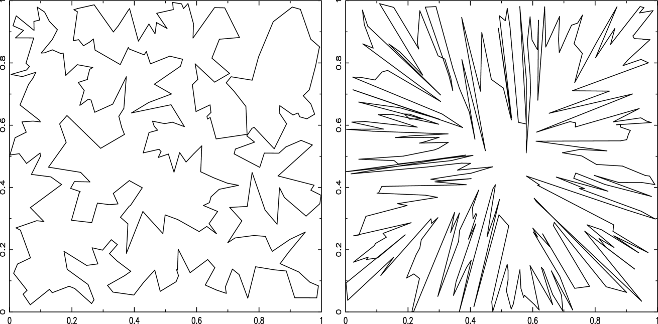
Figure 1: Typical near optimal a priori PTSP tours with $n=300$ for $p=0.5$(left) and $p=0.1$(right), respectively.

The probabilistic traveling salesman problem (PTSP), introduced by Jaillet jaillet1 ; jaillet2 , is an extension of the traveling salesman problem to optimization in the face of unknown data. Whereas all of the cities in the TSP must be visited once, in the PTSP each city only needs to be visited with some probability, $p$. One first decides upon the order in which the cities are to be visited, the ‘a priori’ tour. Subsequently, it is revealed which cities need to be visited, and those which do not need to be visited are skipped to leave a ‘pruned tour’. The order in which the cities are to be visited is preserved when pruning superfluous cities. The objective is to chose an a priori tour which minimizes the average length of the pruned tour. It is clear from figure 1 that near optimal a priori tours may appear very different for different values of $p$.

In our terminology, the average pruned tour length is averaged over all possible instances of which cities require to be visited. This was given by Jaillet as jaillet1

$$\bar{L}_{\text{pruned}}=\sum_{q=0}^{n-2}\ p^{2}(1-p)^{q}\ L_{t}^{(q)}$$ (8)

where

$$L_{t}^{(q)}=\sum_{j=1}^{n}d(j,1+(j+q)_{\mbox{mod}\,n})$$ (9)

is the sum of the distances between each city and its $(q+1)^{th}$ following city on the a priori tour, and the factors $p^{2}(1-p)^{q}$ in the preceding equation simply give the probability that any particular span skipping $q$ cities occurs in the pruned tour.  Jaillet’s closed form expression for the average pruned tour length renders the PTSP to some extent accessible as a standard (but still NP complete) optimization problem, and provides some check on the PTSP results by stochastic optimization methods.

It has been conjectured bertsimas4 that, in the limit of large $n$, the PTSP strategy is as good as constructing a TSP tour on the cities requiring a visit, the re-optimization strategy. This would mean that

$$\lim_{n\rightarrow\infty}\left(\frac{E\left(\bar{L}_{\text{pruned}}\right)}{\sqrt{np}}\right)=\beta_{\text{TSP}},$$ (10)

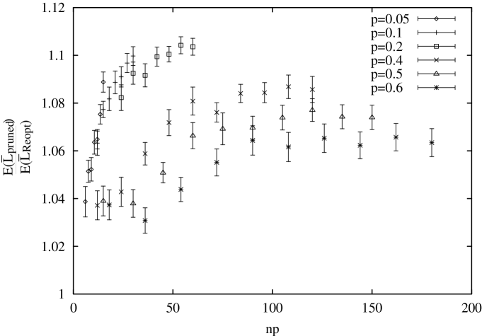
Figure 2: The expected pruned tour length divided by the expected re-optimized tour length. This indicates the improvement one would expect from re-optimization.

where $E(\bar{L}_{\text{pruned}})$ is the pruned tour length further averaged over city positions after optimisation, which we will refer to as the expected pruned tour length.  Figure  2 shows the expected pruned tour length divided by the expected re-optimized tour length. Since this quantity is tending towards a value significantly greater than 1 for $p<1$ it demonstrates that the PTSP strategy can be worse than the re-optimization strategy.  Jaillet jaillet1 and Bertsimas et al. bertsimas2 have also shown that there is a limit to how much worse it can be,  with

$$\lim_{n\rightarrow\infty}\left(\frac{E\left(\bar{L}_{\text{pruned}}\right)}{\sqrt{np}}\right)=\beta_{\text{pruned}}(p)$$ (11)

where

$$\beta_{\text{TSP}}\leq\beta_{\text{pruned}}(p)\leq Min(0.9212,\frac{\beta_{\text{TSP}}}{\sqrt{p}}).$$ (12)

One attempt to solve the PTSP using an exact method was taken by Laporte et al. laporte who introduced the use of integer linear stochastic programming. Although use of algorithms which may exactly solve the PTSP are useful, they are always very limited in the size of problem which may be attempted. Furthermore, the stochastic programming algorithm even fails to solve the PTSP on certain occasions, thus the accuracy of any statistics that would be generated using this method is dubious.

Three studies have used heuristics to solve the PTSP bertsimas1 ; rossi ; bertsimas5 . None of these studies used global search heuristics, and all were very restricted in the problem size attempted due to computational cost. The evaluation of a move for the PTSP using equation 8 involves the computation of $O(n^{2})$ terms compared to $O(1)$ computations to evaluate a move in the TSP. Thus, to solve a 100 city problem for the PTSP would take $O\left(10,000\right)$ times longer than it would to solve a 100 city problem for the TSP. It should be noted, however, that it is only possible to make this comparison due to the relative simplicity of the PTSP. For many more stochastic optimization problems, standard optimization techniques are simply not applicable.

III Form Of The Optimal Tour & Scaling Arguments

Optimal a priori PTSP tours for small $p$, as exemplified in figure 1 for $p=0.1$, resemble an “angular sort” - where cities are ordered by their angle with respect to the centre of the square. Bertsimas bertsimas1 proposed that an angular sort be optimal as $p\rightarrow 0$, but we can show this to be false by comparison to a space-filling curve algorithm which is generally superior as $n\rightarrow\infty$. Such an algorithm was introduced by Bartholdi et al. bartholdi using a technique based on a Sierpinski curve.

For the angular sort with $np\gg 1,$ the probability of two cities being nearest neighbours on the pruned tour will be vanishingly small for cities which are separated from each other by a large angle on the a priori tour. This means that only cities that are separated by a small angle contribute significantly to eq. 8. Thus for an $n$ city tour chosen by angular sort, we may approximate

$$L_{t}^{(q)}\simeq L_{o}n$$ (13)

where $L_{o}$ is some fraction of the side of the unit square, since cities which are sorted with respect to angle will be unsorted with respect to radial distance. This leads to

$$E(\bar{L}_{\text{ang}})\simeq L_{o}np^{2}\sum_{q=0}^{n-2}(1-p)^{q}.$$ (14)

For $np\gg 1$ and $p\ll 1$, we then find that the angular sort yields

$$E(\bar{L}_{\text{ang}})\rightarrow L_{o}np.$$ (15)

By contrast it has been shownbertsimas2 that

$$\frac{E(\bar{L}_{\tau_{\text{sf}}})}{E(\bar{L}_{\text{Reopt}})}=C$$ (16)

with probability 1, where $E(\bar{L}_{\tau_{\text{sf}}})$ is the expected length of a tour generated by a heuristic based on the Sierpinski curve and $E(\bar{L}_{\text{Reopt}})$ is the expected length for the re-optimization strategy. Using previous computational results bertsimas2 ; lee , we estimate $C\simeq 1.33$, which is worse than we achieve using stochastic annealing. Hence, $E(\bar{L}_{\tau_{\text{sf}}})$ is given by

$$E(\bar{L}_{\tau_{\text{sf}}})=O(\sqrt{np})$$ (17)

which leads to

$$\frac{E(\bar{L}_{\tau_{\text{sf}}})}{E(\bar{L}_{\text{ang}})}=O(\frac{1}{\sqrt{np}}).$$ (18)

So for large enough $np$, the angular sort is not optimal.

From inspection of near-optimal PTSP tours such as fig. 1, we propose that the tour behaves differently on different length scales; the tour being TSP-like at larger length scales, but resembling a locally directed sort at smaller length scales. We may construct such a tour and use scaling arguments to analyse both the pruned and a priori lengths of the optimal tour.  Consider dividing the unit square into a series of ‘blobs’, each blob containing $1/p$ cities so that of order one city requires a visit. The number of such blobs is given by

$$N\simeq np$$ (19)

and for these to approximately cover the unit square their typical linear dimension $\xi$ must obey

$$N\xi^{2}\sim 1.$$ (20)

Since each blob is visited of order once by a pruned tour, we can estimate the expected pruned tour length to be

$$E(\bar{L}_{\text{pruned}})\sim N\xi\sim\sqrt{np}$$ (21)

which we will see below is verified numerically. We can similarly estimate the a priori tour length to be $n$ times the distance between two cities in the same blob. Thus, the expected a priori tour length is

$$E\left(L_{\text{a priori}}\right)\sim n\xi\sim\sqrt{\frac{n}{p}}$$ (22)

which is more difficult to confirm numerically.

IV Computational Results For The PTSP

We have investigated near optimal PTSP tours for a range of different numbers of cities, and various values of $p$. We used stochastic annealing with effective temperatures in the range $kT=0.07-0.01$, corresponding to sample sizes in the range $r=2-500$. Between $10$ and $80$ different random city configurations were optimized ($80$ configurations of 30 cities, $40$ configurations of 60 cities, $20$ configurations of 90 cities and $10$ configurations for $n\geq 120$ cities).

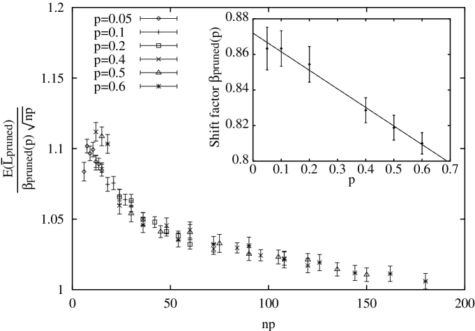
Figure 3: The master curve for the pruned tour length divided by $\beta_{\mbox{pruned}}(p)\sqrt{np}$. The data follows a smooth curve for $n>30$, and the shift factors follow a linear relationship, suggesting that $\frac{E\left(\bar{L}_{\mbox{pruned}}\right)}{\sqrt{np}(0.872-0.105p)}=f(np)$.  Three points with $n=30$ can be seen to fit less well (here and also in fig. 4),  showing breakdown of the master curve at small $n$.

Figure 3 shows a master curve for the expected pruned tour length divided by $\sqrt{np}$. The shift factors have a linear fit and the data are consistent with

$$\frac{E(\bar{L}_{\text{pruned}})}{\sqrt{np}(a-bp)}=f(np)$$ (23)

for $n\gg 1$, where $a=0.872\pm 0.002$, $b=0.105\pm 0.005$ and $f(np)\rightarrow 1$ for large $np$. The shift factors indicate that the PTSP strategy can be no more than $\frac{0.872}{0.767}-1=14\left(\pm 1\right)$ worse than the re-optimization strategy.

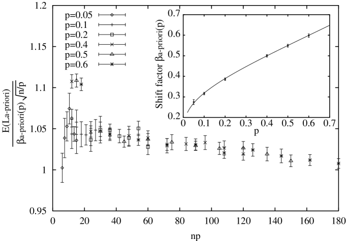
Figure 4: The master curve for the a priori tour length divided by $\sqrt{\frac{n}{p}}\beta_{\mbox{a priori}}(p)$. The shift factors, inset, are expected to tend towards a constant for $p\rightarrow 0$. The slight, but significant, deviation from linear suggests that this might not be the case.

The master curve for the a priori tour length is shown in fig. 4. Our scaling arguments predict that the shift factors $\beta_{\text{a priori}}(p)$ should tend towards a constant for $p\rightarrow 0$. However, data are fit very well by the relation

$$\beta_{\text{a priori}}(p)=\frac{1}{1.25-0.82ln(p)}$$ (24)

which would tend to zero as $p\rightarrow 0$ in conflict with our scaling arguments. To resolve this dilemma we need to probe very small $p$.

V The Limiting Case $p\rightarrow 0$

We are interested in finding whether $\beta_{\text{a priori}}(p)$ tends towards a constant as $p\rightarrow 0$. To do this using the above approach is difficult, since we need a large number of cities to produce reliable data for this regime. Extraction of this behaviour can however be achieved by comparing simulations for different values of $n$, but fixed $np$. We accomplish this by insisting that each instance has 4 cities on the pruned tour. 4 city tours are chosen since they are the smallest for which it matters in which order the cities are visited. This can be viewed as an efficient way to simulate (approximately) the PTSP strategy with $p=\frac{4}{n}$.

Since we are considering the PTSP at fixed $np$, if $\beta_{\text{a priori}}(p)$ tends towards a (non-zero) constant as $p\rightarrow 0$ then we expect $E\left(L_{\text{a priori}}^{\text{4 city}}\right)/n$ to tend towards a constant as $p\rightarrow 0$. Simulations in this regime were performed for $N=12-210$,  with $100$ different random city configurations used for $N<30$, $20$ configurations for $N\leq 90$ and $10$ configurations for $N\geq 120$. Figure 5 shows a linear-log plot of $\frac{n}{2E\left(L_{\text{a priori}}^{\text{4 city}}\right)}$ against $\ln(n/4)\cong\ln(1/p)$. For small $n$ these results reasonably match the direct measurements of $\beta_{\text{a priori}}(p)$, shown for comparison. However,  for surprisingly large $n\sim 100$ which is beyond the range of our $\beta_{\text{a priori}}(p)$ data, our earlier proposal of scaling behaviour is vindicated by $E\left(L_{\text{a priori}}^{\text{4 city}}\right)/n$ approaching a constant value. In summary we have

$$E(L_{\text{a priori}})=\sqrt{\frac{n}{p}}\beta_{\text{a priori}}(p)$$ (25)

where

$$\beta_{\text{a priori}}(p)\left\{\begin{array}[]{ll}=\frac{1}{1.25-0.82\,ln(p)}&\;\;\;\;\;p>0.03\\ =\beta_{0}&\;\;\;\;\;p<0.03.\end{array}\right.$$ (26)

VI Notes on Algorithm Implementation

We applied stochastic annealing to the PTSP using a combination of the 2-opt and 1-shift move-setslin1 established for the TSP. Both move-sets work similarly to that which would be expected for the deterministic case. The expected pruned tour length change for the move was estimated by averaging the change in the tour length for a number of instances. For a given instance it is not necessary to decide whether every city is present, but only the set of cities closest to the move which determine the change in the pruned tour length (see figure 6). For the PTSP, the location of the nearest cities on the pruned tour to the move is determined from a simple Poisson distribution.

When using stochastic optimization, the only variable over which we have control is the sample size (the number of instances) $r$, whereas the effective temperature $\frac{\sigma}{\sqrt{r}}$ also entails the standard deviation $\sigma$ of the pruned length change over instances. As shown in figure 7, annealing by controlling $r$ alone exhibits a relatively sharp transition in the expected pruned tour length. The rapid transition appears to ‘freeze in’ limitations in the tours found (analogous to defects in a physical low temperature phase). By comparison we obtain a much smoother change when $\frac{\sigma}{\sqrt{r}}$ is controlled.

The sharpness of the transition under control by $r$ is caused by the fact that $\sigma$ may vary from move to move, and is on average lower when the expected pruned tour length is less. The jump in the pruned tour length is accompanied by a jump in $\sigma$ and hence the temperature. We suggest that quite generally controlling $\frac{\sigma}{\sqrt{r}}$ gives a better cooling schedule than focussing on $r$ alone.

VII Conclusion

We have shown that earlier incompatible ideas about the form of PTSP tours especially at small $p$bertsimas1 ; bertsimas4 ; bartholdi are resolved by a new crossover scaling interpretation.  The crossover scale corresponds to a group of cities such that of order one will typically have to be visited;  below this scale the (optimsed) a priori PTSP tours resemble a local sort whereas they are TSP-like on scales larger than the crossover. Our computational results for the pruned tour length are summarised by eq. 23 and clearly support the crossover scaling.

Computationally the a priori tour length is more subtle than the pruned tour length,  although it does ultimately conform to expectations from crossover scaling. We introduced 4-city tours to probe the behaviour of a priori tour length down to very small $p$. As summarised by eq. 25,  we find a wide pre-asymptotic regime until  recovering the expected crossover scaling only for $p<0.03$.  Understanding these anomalies in the a priori tour length,  and confirming them analytically, is left as a future challenge.

We have shown stochastic annealing to be a robust and effective stochastic optimization technique,  taking the PTSP as a representative difficult stochastic optimization problem.  In this case it enabled us to obtain representative results out to unprecedented problem sizes,  which in turn supported a whole new view of how the tours behave.  Of relevance to wider applications of stochastic optimmisation,  we have seen that smoother annealing can be obtained by directly controlling the effective temperature$\frac{\sigma}{\sqrt{r}}$fink1 rather than simply the bare depth of sampling $r$ alone.

NEB would like to thank BP Amoco & EPSRC for the support of a CASE award during this research.

The Length of a TSP Tour for small numbers of cities

Numerical estimates of the length of a TSP tour for $n\leq 10$ are given below

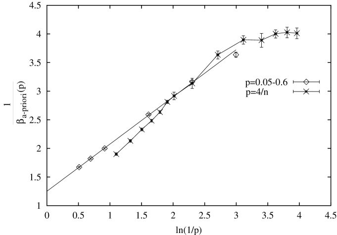
Figure 5: Reciprocal shift factors for a-priori tours (diamonds) compared to estimates from 4 city tours (crosses), $\frac{1}{\beta_{a-priori}(p)}\simeq\frac{n}{2E\left(L_{\text{a priori}}^{\text{4 city}}\right)}$. The 4 city tour data is optimized when each of the instances have 4 cities on the pruned tour. The direct measurements do not appear to saturate within the accessible range of $p$. The crosses show matching behaviour, with saturation at larger $n$ corresponding to inaccessible $p$, suggesting that $E(L_{\mbox{a priori}})=\beta_{0}\sqrt{\frac{n}{p}}$ for small $p$.

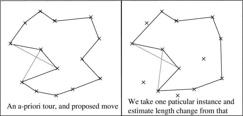
Figure 6: When estimating the expected length change due to a move, we randomly generate instances. Only the cities that are nearest to the move are needed to calculate the change in the pruned tour length.

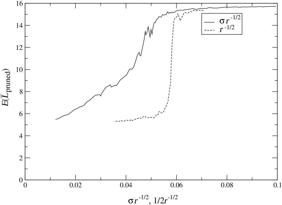
Figure 7: The expected pruned tour length for annealings when $r$ and $1/T=\frac{\sqrt{r}}{\sigma}$ are increased monotonically. The sharp drop in the pruned tour length is seen when only $r$ is controlled, demonstrating that this “freezes in” imperfections in the tour.  The system was annealed at each value of the temperature and value of $r$ for 50,000 Monte Carlo steps with $n=300$ and $p=0.1$.

Number of cities $n$	Number of instances $I$	Average tour length	$\sigma/\sqrt{I-1}$
2	100000	1.043	0.002
3	100000	1.564	0.002
4	5000	1.889	0.006
5	5000	2.123	0.006
6	5000	2.311	0.005
7	5000	2.472	0.005
8	5000	2.616	0.005
9	5000	2.740	0.005
10	5000	2.862	0.005

Table 1: The length of the optimal TSP tour for $n$ cities.

References

- (1) R. C. Ball, T. M. Fink, and N. E. Bowler, submitted to Physical Review Letters, available at http://arXiv.org/abs/cond-mat/0301179 (unpublished).
- (2) T. W. Jonsbraten, Journal of the operational research society 49, 811 (1998).
- (3) H. Robbins and S. Munro, The annals of mathematical statistics 22, 400 (1951).
- (4) A. Benveniste, M. Métivier, and P. Priouret, Adaptive algorithms and stochastic approximation (Springer-Verlag, New York, 1990).
- (5) H. J. Kushner and F. J. Vásquez, SIAM Journal on Control and Optimization 34, 712 (1996).
- (6) P. L’Ecuyer and G. Yin, SIAM Journal on Optimization 8 No. 1, 217 (1998).
- (7) H. J. Kushner, SIAM Journal on Applied Mathematics 47, 169 (1987).
- (8) W. B. Gong, Y. C. Ho, and W. Zhai, in Proceedings of the 31st IEEE conference on decision and control (IEEE, PO Box 1331, Piscataway, NJ, 1992), pp. 795–802.
- (9) D. Yan and H. Mukai, SIAM journal on control and optimization 30 No. 3, 594 (1992).
- (10) L. P. Devroye, IEEE Transactions on Information Theory 24, 142 (1978).
- (11) S. Yakowitz and E. Lugosi, SIAM Journal on Scientific and Statistical Computing 11, 702 (1990).
- (12) S. Andradóttir, SIAM Journal on Optimization 6 No. 2, 513 (1996).
- (13) J. Haddock and J. Mittenthal, Computers and Industrial Engineering 22 No. 4, 387 (1992).
- (14) A. A. Bulgak and J. L. Sanders, in Proceedings of the 1988 Winter Simulation Conference (IEEE, PO Box 1331, Piscataway, NJ, 1988), pp. 684–690.
- (15) M. H. Alrefaei and S. Andradóttir, Management Science 45 No. 5, 748 (1999).
- (16) T. M. A. Khamis, M. A. Ahmed, and V. K. Tuan, European Journal of Operational Research 116 No. 3, 530 (1999).
- (17) W. J. Gutjahr and G. C. Pflug, Journal of global optimization 8, 1 (1996).
- (18) S. B. Gelfand and S. K. Mitter, J. Optimization Theory and Applications 62, 49 (1989).
- (19) S. Rees and R. C. Ball, J. Phys. A 20, 1239 (1987).
- (20) J. D. Nulton and P. Salamon, Phys. Rev. A 37 No. 4, 1351 (1988).
- (21) P. Salamon, J. D. Nulton, J. R. Harland, J. Pedersen, G. Ruppiener, and L. Liao, Computer Physics Communications 49, 423 (1988).
- (22) D. J. Bertsimas, P. Jaillet, and A. R. Odoni, Operations Research 38 No. 6, 1019 (1990).
- (23) J. Beardwood, J. H. Halton, and J. M. Hammersley, Proceedings of the Cambridge Philosophical Society 55, 299 (1959).
- (24) J. M. Steele, Annals of Probability 9, 365 (1981).
- (25) J. Lee and M. Y. Choi, Phys. Rev. E 50, R651 (1994).
- (26) P. Jaillet, Ph.D. thesis, M.I.T., 1985.
- (27) P. Jaillet, Operations research 36, 929 (1988).
- (28) D. J. Bertsimas and L. H. Howell, Eur. J. of Operational Research 65, 68 (1993).
- (29) G. Laporte, F. V. Louveaux, and H. Mercure, Operations research 42 No. 3, 543 (1994).
- (30) D. J. Bertsimas, Ph.D. thesis, M.I.T., 1988.
- (31) F. A. Rossi and I. Gavioli, in Advanced school on stochastics in combinatorial optimization, edited by G. Andreatta, F. Mason, and P. Serafini (World Scientific, Singapore, 1987), pp. 214–227.
- (32) D. J. Bertsimas, P. Chervi, and M. Peterson, Transportation science 29 No. 4, 342 (1995).
- (33) J. J. Bartholdi and L. K. Blatzman, Operations Research Lett. 1, 121 (1982).
- (34) S. Lin, Bell Systems Technological Journal 44, 2245 (1965).