Application of time-dependent density functional theory to electron-vibration coupling in benzene

Abstract

Optical properties of symmetry-forbidden $\pi$-$\pi^{*}$  transitions in benzene are calculated with the time-dependent density functional theory (TDDFT), using an adiabatic LDA functional. Quantities calculated are the envelopes of the Franck-Condon factors of the vibrationally promoted transitions and the associated oscillator strengths. The strengths, which span three orders of magnitude, are reproduced to better than a factor of two by the theory. Comparable agreement is found for the Franck-Condon widths. We conclude that rather detailed information can be obtained with the TDDFT and it may be worthwhile to explore other density functionals.

The time-dependent density functional theory (TDDFT) has proven to be a surprisingly successful theory of excitations and particularly the optical absorption strength function. The theory is now being widely applied in both chemistry and in condensed matter physics. The literature in quantum chemistry is cited in a recent study on the electronic excitations in benzene [1]. Benzene is an interesting molecule for testing approximations because its spectra have been very well characterized, both electronic and vibrational. In this note we will apply the TDDFT to coupling between vibrational and electronic excitations. In our previous studies, we have investigated many different electronic structure questions using a rather simple version of the density functional theory, the local density approximation (LDA). Our emphasis has been to study the overall predictive power of a fixed functional rather than to try to find the best functional for each properties. The approximation scheme we consider is straightforward and uses the same computer programs as for calculating purely electronic excitations. We treat the electronic dynamics in the adiabatic approximation, taking the same energy function for the dynamic equation as is used in the static structure calculation. In our view, this is the only consistent scheme available that guarantees conservation of the oscillator sum rule. The electron-vibration coupling is treated in a vertical approximation, so only information at frozen nuclear coordinates is required.

We consider only spin-singlet states in this work and drop the spin designation in labeling the states. Empirically, the lowest states derive from the $\pi$-$\pi^{*}$  manifold, exciting an electron from the two-fold degenerate $e_{1g}$ HOMO orbital to the two-fold degenerate $e_{2u}$ orbital. The four states consist of a strongly absorbing two-fold degenerate $E_{1u}$ excitation and two other states, $B_{1u}$ and $B_{2u}$, for which symmetry forbids any transition strength. This basic spectrum is shown in Fig. 1, comparing also with our TDDFT calculation, the TDDFT calculation of ref. [1], and the CI theory of ref. [2].

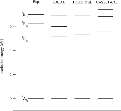
Figure 1: Electronic excitations of benzene in the $\pi$-$\pi^{*}$  manifold. Besides the experimental data and the present TDDFT, we show the TDDFT of ref. [1] and the CI calculation of ref. [2]

It is seen that the TDDFT gives an excellent account of the energies. In fact the TDDFT gives a good description of the higher frequency absorption including $\sigma$-$\sigma^{*}$ transitions as well [3]. The detailed optical properties of the three transitions have been studied gas phase absorption [4, 5]. The strong transition is the $E_{1u}$ with $f=0.9-0.95$. The $B_{1u}$ mode is seen as a shoulder on the strong $E_{1u}$ peak. Its total transition strength is about a factor of 10 lower than the strong state; ref. [4] quotes a value $f=0.09$. The $B_{2u}$ transition is very weak and is seen as a partially resolved set of vibrational transitions with a total strength about $f\approx 1.3\times 10^{-3}$[4]. The strength associated with the most prominent resolved states is $0.6\times 10^{-3}$[5].

The vibrational couplings of the $B$ states has been recently studied using the CASSCF method and analytic expressions for the linear coupling to vibrations[6], and we shall compare with their results. The TDDFT includes correlation effects in a different way, and has some well-known advantages such as the automatic conservation of required sum rules. Also, as mentioned earlier, the present method does not require any reprogramming.

For our treatment of the vibrational motion, we assume that the the vibrations are harmonic in the electronic ground state. The Hamiltonian may be defined

$${\cal H}=-\sum_{i}^{3N}{\hbar^{2}\over 2M_{i}m}{\partial^{2}\over\partial q_{i}^{2}}+\frac{1}{2}\sum_{ij}^{3N}F_{ij}q_{i}q_{j}.$$ (1)

where $q_{i}$ are the 36 Cartesian displacement coordinates of the 12 atomic centers, $m$ is the atomic mass unit, $M_{i}$ is the mass of the atom in daltons, and $F_{ij}$ is the matrix of force constants. The matrix ${\bf M}^{-1/2}{\bf F}{\bf M}^{-1/2}$ (M is the diagonal matrix of masses $M_{i}$) is diagonalized by an orthogonal transformation ${\bf U}$ to obtain the normal modes $Q_{k}$ and the eigenfrequencies $\omega_{k}=2\pi\nu_{k}$. The Cartesian displacements are obtained directly from the rows of the transformation matrix ${\bf U}$, $q_{i}=M^{-1/2}_{i}\sum_{k}U_{ik}Q_{k}$. The translational and rotational motions will also be contained in the transformation matrix ${\bf U}$ as zero frequency modes. The probability distribution of the zero point motion is then given simply by

$$P({\vec{Q}})\sim\exp(-\sum_{k}Q_{k}^{2}/2Q_{0k}^{2}).$$ (2)

where

$$Q_{0k}=\sqrt{{\hbar\over 2m\omega_{k}}}={4.1\hbox{[\AA]}\over\sqrt{n_{cm}}}$$

is the r.m.s. amplitude of the zero-point motion. The last equality expresses the formula in common units with $n_{cm}=c/\nu$ the energy of the vibration in wavenumbers [cm^-1].

The optical absorption strength function in the presence of the zero point motion is determined by the convolution the probability distribution of displacements with the strength calculated as a function of displacement,

$$f=\int d^{N}Q_{k}P({\vec{Q}})f({\vec{Q}}).$$ (3)

We thus need the absorption strength as a function of the normal mode coordinates $Q_{k}$. In the case of a forbidden transition promoted by the vibration $k$, the coupling is linear for small displacements and the transition strength will be quadratic in $Q_{k}$,

$$f(Q_{k})=f_{0k}{Q_{k}^{2}\over Q_{0k}^{2}}+...$$ (4)

We verify below that this functional dependence is satisfied for the couplings of interest in benzene. Then the convolution over the ground state probability distribution gives simply $f=f_{0k}$.

We also consider widths of the transitions due to the Franck-Condon factors of multiply excited vibrations. This is calculated by replacing $f$ with the strength function $S(E,Q)=f(Q)\delta(E-E(Q))$ in eq. 3. Assuming that the excitation energy is linear in $Q$,

$$E(Q_{k})\approx E_{0}+K_{k}Q_{k}/Q_{0k}+...$$

the Gaussian probability distribution $P$ gives a Gaussian envelope for the Franck-Condon factors,

$$P(E)\sim\exp(-(E-E_{0})^{2}/2K_{k}^{2}).$$ (5)

For the numerical studies reported here, we constructed the transformation matrix ${\bf U}$ using the empirical force field of Goodman and Ozkabak [7], which fits the observed frequencies extremely well. Ab initio calculations of the force field have also reached a high level of accuracy [9]. However, as mentioned earlier, we do not make our own DFT calculations of the force constants because our goal is the dynamic behavior of the electrons. The frequencies and symmetries of the normal modes are listed in Table 1, taken from ref. [7]. The most important modes for the induced transition strengths are the $E_{2g}$ and the $B_{2g}$ modes. The $E_{2g}$ vibrations couple the strong electronic excitation to the other states in the $\pi$-$\pi^{*}$  manifold. The $B_{1g}$ can induce out-of-plane dipole strength for these excitations. The theoretical widths of the excitations are largely due to mode 1, which is an $A_{1g}$ radial oscillation mode that favors carbon displacements. In Fig. 2 we show the Cartesian displacements associated with the two strongest $E_{2g}$ modes with respect to carbon displacements.

Figure 2: Cartesian displacements of the vibrational modes 6a (left) and 8a (right). These modes have symmetry $E_{2g}$ and give the most important couplings for our purposes. The r.m.s. displacement of the atoms are magnified by a factor 40, i.e. $Q_{k}=40Q_{0k}$ with respect to the scale for the equilibrium positions.

The present TDDFT calculations were performed making use of the same representation of the Kohn-Sham operator as in our previous study of the full energy distribution in optical absorption [3]. The wave functions are represented on a coordinate-space mesh as has been introduced in condensed matter physics [ch??]. However, the algorithm in the present program is a new one [10] that uses the conjugate gradient method to extract individual states rather that the direct real-time propagation of the wave function. While the real-time method is very efficient for calculating the global strength function, it is less suited for locating individual eigenstates when they are weakly excited by the dipole operator. In both methods, the electronic ground state for a given nuclear geometry is first computed with the Kohn-Sham equation,

$$-{\nabla^{2}\over 2m}\phi_{i}+{\delta{\cal V}\over\delta n}\phi_{i}=\epsilon_{i}\phi_{i}.$$

We use a simple LDA energy density functional [12] for the electron-electron interaction in ${\cal V}$ and a pseudopotential approximation [13, 14] to treat the interaction of the valence electrons with the ions. The important numerical parameters in the calculation are the the mesh spacing, taken as $\Delta x=0.3$ Å, and the volume in which the wave functions are calculated, which we take as a sphere of radius 7 Å. With these parameters, orbital energies are converged to better than 0.05 eV.

Figure 3: Dependence of the oscillator strength of the ${}^{1}B_{2u}\leftarrow^{1}A_{1g}$ transition on the vibrational coordinate for the 8a mode.

Figure 4: Dependence of the ${}^{1}B_{1u}\leftarrow^{1}A_{1g}$ transition energy on the vibrational coordinate for the mode 1.

Next the TDDFT equations are solved in an representation similar to the RPA equations,

$$-{\nabla^{2}\over 2m}\phi_{i}^{\pm}+{\delta{\cal V}\over\delta n}\phi_{i}^{\pm}-\epsilon_{i}\phi_{i}+{\delta^{2}{\cal V}\over\delta n^{2}}\delta n\phi_{i}=(\epsilon_{i}\pm\omega)\phi_{i}^{\pm}.$$

Here the transition density $\delta n$ and normalization are given by

$$\delta n=\sum_{i}\phi_{i}(\phi_{i}^{+}+\phi_{i}^{-}),\hbox{~{}~{}~{}}\langle\phi_{i}^{+}|\phi_{i}^{+}\rangle-\langle\phi_{i}^{-}|\phi_{i}^{-}\rangle=1.$$

The equations are solved by the conjugate gradient method for the generalized eigenvalue problem [11]. In Fig. 4 we show the dependence of transition strengths $f$ and excitation energies $\omega$ on the coordinates of two of the normal modes. We see that the conditions for applying eq. (4) and (5) are reasonably well satisfied. We may then extract the transition strength $f_{0k}$ and the width $K_{k}$ by fitting the $Q_{k}$-dependence of these quantities. The results for the symmetry-allowed vibrations are shown in shown in Table 2.

We first discuss the widths. The empirical values were obtained by making a three-term Gaussian fit to the absorption data of ref. [15]. The only vibrations that contribute in lowest order are the two $A_{1g}$ breathing modes. The vibrations affect all three transitions identically; mode 1 has the larger amplitude of displacement of the carbon atoms and gives the greater contribution. The results agree rather well with the empirical widths. The magnitude of the widths and its independence of the electronic state can be understood in very simple terms with the Hueckel model. This is to be expected, since the excitation energy of the electronic states is mainly due to the orbital energy difference, and that is describe quite well by the Hueckel model. For benzene, the energy difference is related to the hopping matrix element $\beta$ by $E_{LUMO}-E_{HOMO}=2\beta.$. Allowing changes in the nuclear coordinates, the hopping matrix element will depend on the distance between neighboring atoms $d$; this may be parameterized by the form

$$\beta(d)=\beta_{0}\left({d_{0}\over d}\right)^{\alpha}.$$

Then the HOMO-LUMO gap fluctuates due to the breathing mode vibrations with widths given by

$$\Delta E=2\beta_{0}\alpha{\Delta r\over r}$$

where $r$ is the radial distance of the carbons from the center and $\Delta r$ is at $Q_{k}=Q_{0k}$ in an $A_{1g}$ mode. From fitting orbital energies in various conjugated carbon systems one may extract values $\alpha\approx 2.7$ and $\beta_{0}=2.5$ eV[3]. Inserting these values in the above equation, one obtains 0.145 eV for the widths associated with mode 1, quite close to the values obtained by TDDFT. We have included in the table also the r.m.s. widths of the Franck-Condon factors obtained by the CASSCF theory, which gives quite similar results. One thing should be remarked on the comparison with experiment. While the theory gives practically identical widths for all three states, the experimental strength is significantly narrower for the the $E_{1u}$ excitation, and this seems to not be understandable in the TDDFT.

Next we examine the transition strengths of the $B$-transitions induced by the zero-point vibational motion. In the middle table of Table 2 we show the contributions by the six active vibrational modes. The main contribution for the $B_{2u}$ transition comes from mode 6. This is also found in the CASSCF theory, and is how the observed spectrum was interpreted in [5]. In the case of the $B_{1u}$ excitation, the TDDFT predicts that the coupling of mode 8 is dominant. Experimentally, the situation is unclear because the vibrational spectrum of the excited state is strongly perturbed. Ref. [5] assigns both mode 6 and mode 8 vibrational involvement. Irrespective of the spectrum of the vibrational modes in the excited state, the total transition strength is given by the same convolution of the ground state vibrational wave function. As in the case of the widths, the induced $B_{1u}$ transition strength can be understood roughly with the tight-binding model. The charge densities are displaced in the vibration, giving the $B_{1u}$ configuration an induced dipole moment just from the atomic geometry. The Hueckel Hamiltonian of the orbital energy is also affected by the changed separations between carbons, and that cause a violation of the $B_{1u}$ symmetry. Finally, the Coulomb interaction, which is mainly responsible for the splitting of the three electronic states, is affected by the changed separations. Of these three mechanisms, only the effect of the symmetry-violation in the Hueckel Hamiltonian is important, and mode 8 crries the largest flutuation in $d$. Taking the same $d$-dependence as before, the strength obtained in the tight-binding model is 0.05, rather close to the TDDFT result. The tight-binding model cannot be used to estimate the very weak $B_{2u}$ transition because the charge density on the atoms is identically zero.

The lower table gives the empirical transition strengths [4] and comparison to theory. The agreement between theory and experiment is quite good for all states. For the weakest transition, the $B_{1u}$, the TDDFT gives a transition strength 25% higher than the empirical For the case of the $B_{1u}$ transition, the TDDFT prediction is within 35% of the measured value. We also show the previously reported value for the $E_{1u}$ which is within 20%. We consider this remarkable success of the TDDFT considering that the strengths that range over three orders of magnitude.

In conclusion, we have shown that the TDDFT gives a semiquantitative account of the effect of zero-point vibrational motion on the optical absorption spectrum in benzene. In this respect this extends the possible domain of utility from the region of infrared absorption, where it is known that the TDDFT gives a description of transition strengths accurate to a factor of two or so[16]. We are encouraged by these results to apply the TDDFT to other problems involving the electron-vibrational coupling. Perhaps it should be mentioned that not all excitation properties are reproduced so well in the TDDFT. In particular, one can not expect accurate numbers for HOMO-LUMO gap of insulators [18] and the optical rotatory power of chiral molecules [19]. Of course, there may be better energy functionals for studying particular properties, and it might be interesting to examine theories including gradient terms in the functional.

We acknowledge stimulating discussions with G. Roepke. This work was supported by the Department of Energy under Grant DE-FG06-90ER40561.

mode	species	$\bar{\nu}_{\rm obs}\;[{\rm cm}^{-1}]$	mode	species	$\bar{\nu}_{\rm obs}\;[{\rm cm}^{-1}]$
1	$A_{1g}$	993.1	9	$E_{2g}$	1177.8
2	$A_{1g}$	3073.9	18	$E_{1u}$	1038.3
3	$A_{2g}$	1350	19	$E_{1u}$	1484.0
12	$B_{1u}$	1010	20	$E_{1u}$	3064.4
13	$B_{1u}$	3057	11	$A_{2u}$	674.0
14	$B_{2u}$	1309.4	4	$B_{2g}$	707
15	$B_{2u}$	1149.7	5	$B_{2g}$	990
6	$E_{2g}$	608.1	10	$E_{1g}$	847.1
7	$E_{2g}$	3056.7	16	$E_{2u}$	398
8	$E_{2g}$	1601.0	17	$E_{2u}$	967

Table 1: The 20 normal modes of vibration of benzene, numbered according to Wilson [17], with their symmetry and observed frequency. The data of this table are taken from [7] where other references can also be found.

Width	$A_{1g}$ vibrations			CASSCF	Exp.
$K_{k}$ (ev)	1	2	Tot.
${}^{1}B_{2u}$	0.12	0.03	0.15	0.14	0.18
${}^{1}B_{1u}$	0.12	0.03	0.15	0.14	0.17
${}^{1}E_{1u}$	0.12	0.03	0.15		0.125

$f_{0k}/10^{-3}$	$B_{2g}$ vib.		$E_{2g}$ vibrations
TDDFT	4	5	6	7	8	9	Total
${}^{1}B_{2u}$	-	-	1.4	0.2	-	-	1.6
${}^{1}B_{1u}$	-	1.6	0.4	-	44.	13.	59

$f/10^{-3}$	TDDFT	CASSCF	Exp.
${}^{1}B_{2u}$	1.6	0.5	1.3
${}^{1}B_{1u}$	59	75	90
${}^{1}E_{1u}$	1100		900-950

Table 2: Vibrational coupling properties in benzene molecule. The upper table shows the predicted r.m.s. widths associated with the breathing mode vibrations. The total is compared to the CASSCF calculation of ref. [6] and to experiment (see text). In the middle table, the predicted transition strength associated with the various vibrations are given, with blank entries having values smaller than $10^{-4}$. In the lower table, the predicted total transition strength is compared with the CASSCF theory and to experiment [4].

References

- [1] H. Heinze, A. Goerling, and N. Roesch, J. Chem. Phys. 113 2088 (2000).
- [2] J. Mauricio O. Matos, B. O. Roos, and P-Å Malmqvist, J. Chem. Phys. 86, 3 (1987).
- [3] K. Yabana, and G. F. Bertsch, Int. J. Quant. Chem. 75, 55 (1999).
- [4] E. Pantos, J. Philis, A Bolovinos, Jour. Mol. Spectro. 72 36 (1978).
- [5] A. Hiraya and K. Shobatake, J. Chem. Phys. 94 7700 (1991).
- [6] A. Bernhardsson, et al., J. Chem. Phys. 112 2798 (2000).
- [7] L. Goodman, A. G. Ozkabak, and S. N. Thakur, J. Phys. Chem. 95, 9044 (1991).
- [8] J. Chelikowsky, et al., Phys. Rev. 50 11355 (1994).
- [9] J. M.L. Martin, P. R. Taylor, and T. J. Lee, Chem. Phys. Lett. 275, 414 (1997) (and refs. therein).
- [10] K. Yabana, to be published.
- [11] W.W. Bradbury and R. Fletcher, Num. Math. 9 259 (1966).
- [12] J. Perdew and A. Zunger, Phys. Rev. B23 5048 (1981).
- [13] N. Troullier and J.L. Martins, Phys. Rev. B43 1993 (1991).
- [14] L. Kleinman and D. Bylander, Phys. Rev. Lett. 48 1425 (1982).
- [15] H.-H. Perkampus, UV Atlas of organic compounds, (Vol. 1, Butterworth Verlag Chemie, 1968).
- [16] G.F. Bertsch, A. Smith, and K. Yabana, Phys. Rev. B52 7876 (1995).
- [17] E. B. Wilson Jr., J. C. Decius, and Paul C. Cross, Molecular Vibrations, (McGraw-Hill, New York, 1955).
- [18] L. Hedin, J. Phys. Condens. Matter 11 R489 (1999).
- [19] K. Yabana and G.F. Bertsch, Phys. Rev. A60 1271 (1999).