Abstract

Quantum Gravity is quite elusive at the experimental level; thus a lot of interest has been raised by recent searches for quantum gravity effects in the propagation of light from distant sources, like gamma ray bursters and active galactic nuclei, and also in earth-based interferometers, like those used for gravitational wave detection. Here we describe a simple heuristic picture of the quantum fluctuations of the gravitational field that we have proposed recently, and show how to use it to estimate quantum gravity effects in interferometers.

1 Introduction

The propagation of light in random or fluctuating media has long been used as a probe of their statistical properties [1]. This holds true also for exotic media like the background of gravitational waves in the space between the earth and some faraway light source [2, 3, 4] (see figure 1).

Recently several authors have proposed searches for quantum gravity effects in the propagation of light over cosmological distances or in earth-based interferometers; for instance, according to Ellis, Mavromatos and Nanopoulos [5], the vacuum of quantum gravity should be dispersive and this should show up as an energy-dependent spread in the arrival times of energetic photons from distant sources like gamma-ray bursters, active galactic nuclei, and gamma-ray pulsars. This opens up interesting observational opportunities for experimentalists (see, e.g. [6, 7]), but requires either a violation of Lorentz invariance or of the equivalence principle [8].

The proposal [5] is based on the latest developments of $D$-brane theory, and it is yet another picture of the “space-time foam” first proposed by Wheeler in 1957 [9], and later considered by other authors such as Hawking [10].

Here we propose a heuristic treatment of these background fluctuations, which is based on the direct use of the uncertainty principle for energy and time, with additional assumptions on the dynamic and statistical behaviour of the resulting quantum fluctuations. Afterwards we use this model to evaluate the spectral properties of the fluctuations of the energy density and of the gravitational potential, and to derive the behaviour of light in a generic two-arm interferometer.

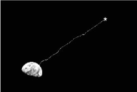
Figure 1: In addition to atmospheric scintillation we expect scintillation effects due to the background of gravitational waves that affect starlight as it travels to the earth. The light emitted by a star does not travel in a straight line, but is scattered by this background: therefore it displays angular displacement and the time of arrival fluctuates randomly.

 

P. Bergmann [2] originally suggested to search for low-frequency components of gravitational waves by attempting to detect fluctuations in the intensity of light, but actually most searches for this effect have been carried out looking for fluctuations in the arrival times of pulses from millisecond pulsars and other such sources. See [3] for the details of how one such search is performed, and [4] for a recent review.

2 Fluctuations of the
gravitational energy density

We consider now a single quantum fluctuation of the vacuum energy density and assume that it is uniformly spread over a spherical region, then the total energy associated with the fluctuation is

$$E=\frac{{4\pi R_{0}^{3}}}{{3}}\rho,$$ (1)

where $R_{0}$ is the radius of the bubble. We assume that the bubble expands at the speed of light, so that $R_{0}=ct$, where $t$ is the time of creation of the bubble, and that it satisfies the time-energy uncertainty principle at all times, so that $E\approx\hbar t$, and therefore we find

$$\rho\approx\frac{{3\hbar}}{{4\pi c^{3}t^{4}}}.$$ (2)

It is also important to note that the expanding bubbles are just a representation of the light cones in $3$-space, therefore they are Lorentz invariant, i.e., they would look the same in any other Lorentz-boosted reference frame. A rough form of Lorentz invariance is thus present in our model, whose causal structure is compatible with a relativistic model of spacetime, and these fluctuations satisfy the requirement, first discussed by Zeldovich [12], that the quantum vacuum must indeed be Lorentz invariant.

Now let $n\left({\vec{x},t}\right)$ be the number density of the fluctuations that occur in spacetime, i.e., $n\left({\vec{x},t}\right)dVdt$ fluctuations are created in a small space-time volume $dVdt$ at position $\vec{x}$ and time $t$, and assume that $n\left({\vec{x},t}\right)dVdt$ is a Poisson variate with average $n_{0}dVdt$ and variance $n_{0}dVdt$ (see fig. 2); then the average density observed at $\left({\vec{x}_{0},t}\right)$ and due to the fluctuations created at a distance r and at an earlier time $t^{\prime}$ is

$$d^{2}\rho=\frac{{3\hbar n_{0}}}{{c^{3}\left({t-t_{0}}\right)}}r^{2}drdt.$$ (3)

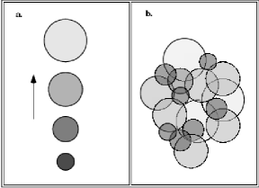
Figure 2: a. We picture the fluctuations of the gravitational energy density as “bubbles” that expand at the speed of light, and are uniformly filled with a decreasing energy density that satisfies at all times the time-energy uncertainty principle; b. an observer sees the whole of space seething with bubbles, whose number density in a given space-time volume follows a simple Poisson statistics. More pictures and simulations of these fluctuations can be found on the web [11].

 

Then the total energy density observed at $\left({\vec{x}_{0},t}\right)$ and due to all the prior fluctuations in the light-cone of the observer is given by

$$\rho_{\mathrm{tot}}\left({t}\right)\approx\int_{r_{\mathrm{min}}}^{r_{\mathrm{max}}}{dr\int_{-T_{0}}^{t-r/c}{dt_{0}\frac{{3\hbar n_{0}}}{{c^{3}\left({t-t_{0}}\right)}}r^{2}}}\approx\hbar n_{0}\ln\frac{{r_{\mathrm{max}}}}{{r_{\mathrm{min}}}},$$ (4)

where $T_{0}$ is the age of the Universe, and $r_{\mathrm{min}}$, $r_{\mathrm{max}}$ are the minimum and the maximum distance from the observer. Furthermore in (4) we have dropped the $\vec{x}$ dependence, because we assume translational invariance. The maximum distance can be taken to be the present radius of the Universe $r_{\mathrm{max}}\approx{{c}\mathord{\left/{\vphantom{{c}{H}}}\right.\kern-1.2pt}{H}}$, while the minimum radius corresponds to the smallest bubble that can possibly be observed, that is that bubble that emerges from a “mini black hole” stage and turns into a “normal” fluctuation, so that $r_{\mathrm{min}}$ is just the Schwartzschild radius of the fluctuation:

$$r_{\mathrm{min}}=\frac{{2G}}{{c^{2}}}\cdot\frac{{E}}{{c^{2}}}\approx\frac{{2G}}{{c^{2}}}\cdot\frac{{\hbar}}{{c^{2}t}}=\frac{{2G\hbar}}{{c^{3}r_{\mathrm{min}}}}.$$ (5)

We solve eq. (5) and find

$$r_{\mathrm{min}}=\sqrt{\frac{{2G\hbar}}{{c^{3}}}},$$ (6)

which is just the Planck length. Thus eq. (4) gives an average density

$$\rho_{\mathrm{tot}}\approx\frac{{1}}{{2}}\hbar n_{0}\ln\frac{{c^{5}}}{{2G\hbar H^{2}}}\quad.$$ (7)

It is worthwhile to notice that a minimum and a maximum scale show up naturally in the calculations, and that the total energy density (7) is seamlessly related to both the micro and the macrostructure of the Universe.

The same formalism can be used to estimate the variance of the energy density fluctuations, and proceeding as before one finds

$$\sigma_{\rho}^{2}=\frac{{9\hbar^{2}cn_{0}}}{{28\pi}}\int_{r_{\mathrm{min}}}^{r_{\mathrm{max}}}{\frac{{dr}}{{r^{5}}}}=\frac{{9\hbar^{2}cn_{0}}}{{112\pi}}\left({\frac{{1}}{{r_{\mathrm{min}}^{4}}}-\frac{{1}}{{r_{\mathrm{max}}^{4}}}}\right)\approx\frac{{9c^{7}n_{0}}}{{448G^{2}\pi}}.$$ (8)

It is also important to notice that the average energy density (7) contributes to the effective cosmological constant [13]:

$$\Delta\Lambda\left({t}\right)=\frac{{8\pi}}{{c^{4}}}G\rho_{\mathrm{tot}}\approx\frac{{8\pi}}{{c^{4}}}G\hbar n_{0}\ln\frac{{c}}{{\ell_{P}H\left({t}\right)}};$$ (9)

recent observations favour a nonzero and positive cosmological constant [14, 15] such that $\Omega_{\Lambda}\approx 0.7$ and $\Lambda=3\Omega_{\Lambda}{{H^{2}}\mathord{\left/{\vphantom{{H^{2}}{c^{2}}}}\right.\kern-1.2pt}{c^{2}}}$; this means that we can use (9) to estimate the order of magnitude of the free parameter $n_{0}$, if we assume that most of the effective cosmological constant is due to the fluctuations considered here:

$$n_{0}\approx\frac{{3\Omega_{\Lambda}H^{2}c^{2}}}{{4\pi G\hbar\ln\left({{{c^{5}}\mathord{\left/{\vphantom{{c^{5}}{2G\hbar H^{2}}}}\right.\kern-1.2pt}{2G\hbar H^{2}}}}\right)}}\approx 3\cdot 10^{22}\,\mathrm{m}^{-3}\mathrm{s}^{-1}.$$ (10)

3 Fluctuations of the gravitational potential

Since we assume that fluctuations spread with the speed of light, there can be no gravitational potential outside the bubble, because for an external observer there is no way to know that it exists, while inside the bubble we assume that the gravitational potential is just the (Newtonian) potential of a sphere of uniform energy density $\rho$:

$$\Phi\left({r}\right)=\cases{\displaystyle-\frac{4\pi G\rho}{3c^{2}}\left(\frac{3}{2}R_{0}^{2}-\frac{1}{2}r^{2}\right)\qquad&if $\quad r<R_{0}$\cr\cr 0&if $\quad r>R_{0}$}.$$ (11)

Integrating as in the case of the energy density one finds:

$$\Phi_{\mathrm{tot}}\approx-\frac{{16\pi G\hbar n_{0}}}{{3c^{2}}}r_{\mathrm{max}}^{2}\approx-\frac{{16\pi G\hbar n_{0}}}{{3cH}}$$ (12)

and

$$\sigma_{\Phi}^{2}=\frac{{68\pi G^{2}\hbar^{2}n_{0}}}{{35c^{3}}}\ln\frac{{r_{\mathrm{max}}}}{{r_{\mathrm{min}}}}.$$ (13)

4 Correlation functions

A somewhat more complicated integration yields the correlation function of the gravitational potential:

$$\left\langle{\Delta\Phi\left({\vec{x}_{1},t_{1}}\right)\Delta\Phi\left({\vec{x}_{2},t_{2}}\right)}\right\rangle=\left({\frac{{G\hbar c}}{{2c^{2}}}}\right)^{2}n_{0}\int\limits_{S}d^{3}x\int\limits_{t<t^{\star}}dt\left({3-\frac{{r_{1}^{2}}}{{c^{2}\left({t_{1}-t}\right)^{2}}}}\right)\times$$

$$\qquad\times\left(\frac{1}{c^{2}\left(t_{1}-t\right)^{2}}\right)\left({3-\frac{{r_{2}^{2}}}{{c^{2}\left({t_{2}-t}\right)^{2}}}}\right)\left({\frac{{1}}{{c^{2}\left({t_{2}-t}\right)^{2}}}}\right),$$ (14)

where the shorthand notation $r_{1,2}=\left|{\vec{x}_{1,2}-\vec{x}}\right|$ has been used,

$$t^{\star}=\min\left(t_{1}-r_{1}/c,t_{2}-r_{2}/c\right)$$

and S is the range of acceptable values of $\vec{x}_{1,2}$ — i.e., values such that $r_{\mathrm{min}}<r_{1,2}<r_{\mathrm{max}}$.

The expression (14) can be calculated for different special cases, e.g., the time correlation function at a given space point is

$$R\left({\tau}\right)=\left\langle{\Delta\Phi\left({\vec{x},0}\right)\Delta\Phi\left({\vec{x},\tau}\right)}\right\rangle\approx\frac{{68}}{{35}}\frac{{G^{2}\hbar^{2}\pi}}{{c^{3}}}n_{0}\ln\frac{{r_{\mathrm{max}}+c\tau}}{{r_{\mathrm{min}}+c\tau}}$$ (15)

and then, using the Wiener-Kintchine theorem, one finds

$$\left\langle{\left|{\Delta\Phi\left({f}\right)}\right|^{2}}\right\rangle=\int_{-\infty}^{-\infty}{R\left({\tau}\right)\mathrm{e}^{-2\pi\mathrm{i}f\tau}d\tau}\approx\frac{{34}}{{35}}\frac{{G^{2}\hbar^{2}n_{0}\pi}}{{c^{3}}}\cdot\frac{{1}}{{f}}.$$ (16)

5 Irradiance fluctuations
in a two-arm interferometer

In the weak field approximation the frequency of light is linearly related to the gravitational potential

$$\nu\left({\vec{x},t}\right)\approx\nu_{0}\left({1-\frac{{\Phi\left({\vec{x},t}\right)}}{{c^{2}}}}\right);$$ (17)

therefore, using the correlation function (14), one finds that the time correlation function for the irradiance fluctuations in a two-arm interferometer is

$$R_{I}\left({\tau}\right) = \left\langle{\Delta I\left({t}\right)\Delta I\left({t+\tau}\right)}\right\rangle$$ (18)

$$= \frac{{4I_{1}I_{2}\nu_{0}^{2}sin^{2}\varphi_{0}}}{{c^{6}}}\int\!\!\!\int\limits_{L_{1},L_{2}}d\ell_{1}d\ell_{2}\times$$

$$\qquad\times\left\langle{\Phi\left[{\vec{x}\left({\frac{{\ell_{1}}}{{c}}}\right),\frac{{\ell_{1}}}{{c}}}\right]\Phi\left[{\vec{x}\left({\frac{{\ell_{2}}}{{c}}+\tau}\right),\frac{{\ell_{2}}}{{c}}+\tau}\right]}\right\rangle,$$

where $\ell_{1,2}$ is the position along the path $L_{1,2}$, $\nu_{0}$ is the frequency of light in a zero-potential region, $I_{1,2}$ is the irradiance of light along each path, and $\varphi_{0}$ is the average phase difference.

We plan to complete the calculation of the time correlation function (18) for specific interferometer designs in the near future.

References

- [1] Sheng P (ed.) Scattering and Localization of Classical Waves in Random Media, Singapore, World Scientific, 1990
- [2] Bergmann P (1971) Phys. Rev. Lett. 26 1398
- [3] Romani R W and Taylor J H (1983) Astrophys. J. 265 L35
- [4] Giovannini M “Stochastic GW Backgrounds and Ground Based Detectors” in CAPP-2000, AIP Conference Proceedings (to appear)
- [5] Ellis J, Mavromatos N E and Nanopoulos D V (2000) Gen. Rel. Grav. 32 127
- [6] Biller S et al. (1999) Phys. Rev. Lett. 83 2108
- [7] Schaefer B E (1999) Phys. Rev. Lett. 82 4964
- [8] Mavromatos N E gr-qc/0009045
- [9] Wheeler J A (1957) Ann. Phys. 2 604
- [10] Hawking S W (1996) Phys. Rev. D53 3099
- [11] http://www.fisica.uniud.it/milotti/stf/index.html
- [12] Zeldovich Ya B (1968) Sov. Phys. Uspekhi 11 381
- [13] Weinberg S (1989) Rev. Mod. Phys. 61 1
- [14] Schmidt B et al. (1998) Astrophys. J. 507 46
- [15] Perlmutter S et al. (1999) Astrophys. J. 517 565