Wannier-Stark states of a quantum particle in 2D lattices

Abstract

A simple method of calculating the Wannier-Stark resonances in 2D lattices is suggested. Using this method we calculate the complex Wannier-Stark spectrum for a non-separable 2D potential realized in optical lattices and analyze its general structure. The dependence of the lifetime of Wannier-Stark states on the direction of the static field (relative to the crystallographic axis of the lattice) is briefly discussed.

I Introduction

The quantum states of a particle in a periodic potential plus homogeneous field (known nowadays as the Wannier-Stark states, WS-states in what follows) are one of the long-standing problems of single-particle quantum mechanics. The beginning of the study of this problem dates back to the paper by Bloch of 1929, followed by contributions of Zener, Landau, Wannier, Zak and many others history . In the late eighties the problem got a new impact by the invention of semiconductor superlattices. The unambiguous observation of the WS-spectrum in a semiconductor superlattice mendez ended a long theoretical debate about the nature of WS-states, and now it is commonly accepted that they are the resonance states of the system. Besides, WS-states were recently studied in a system of cold atoms in an optical lattice atoms and some other (quasi) one-dimensional systems.

Although WS-states are resonances, i.e. metastable states, in the theoretical analysis of related problems they were usually approximated by stationary states (one-band, tight-binding, and similar approximations). Beyond the one-band approximation, WS-states in the semiconductor and optical lattices were studied in recent papers preprint and papers by using the scattering matrix approach of Ref. PRL1 (see also Ref. JOB2 for details). This approach actually solves the one-dimensional Wannier-Stark problem and supplies exhaustive information about 1D WS-states. In the present letter we extend the method of Ref. PRL1 ; JOB2 to the case of two-dimensional lattices. For the first time we find the complex spectrum of 2D WS-states and analyze its general structure.

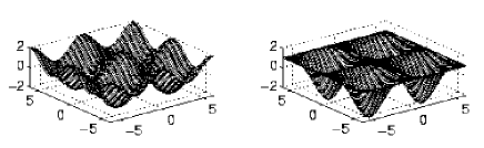
Figure 1: Potential energy (2) for $\epsilon=0$ (a) and $\epsilon=1$ (b).

To be concrete, we choose the following system:

$$H={\bf p}^{2}/2+V({\bf r})+{\bf F}\cdot{\bf r}\;,\qquad{\bf r}=(x,y)\;,$$ (1)

$$V({\bf r})=\cos x+\cos y-\epsilon\cos x\cos y\;,$$ (2)

where $0\leq\epsilon\leq 1$ hbar . Two limiting cases $\epsilon=0$ and $\epsilon=1$ correspond to an ‘egg crate’ potential, for which the system is separable, and a ‘quantum well’ potential, where the coupling between two degrees of freedom is maximal (see Fig. 1). Let us also note that the choice $\epsilon=1$ corresponds to a 2D optical potential created by two standing laser waves crossing at right angle. Thus the results presented below can be directly applied to the system of cold atoms in a 2D optical lattice.

II 2D Wannier-Bloch spectrum

We briefly recall the key points of the 1D theory. The spectrum of the Bloch particle in the presence of a static field consists of several sets of equidistant levels

$${\cal E}_{\alpha,l}=E_{\alpha}+2\pi Fl-{\rm i}\Gamma_{\alpha}/2\;,$$ (3)

known as Wannier-Stark ladders of resonances. In Eq. (3), $2\pi$ stands for the lattice period, $F$ is the amplitude of the static force, $l=0,\pm 1,\dots$ is the site index and the index $\alpha=0,1,\ldots$ labels different ladders. The lifetime of WS-states $\Psi_{\alpha,l}(x)$ is defined by the resonance width $\Gamma_{\alpha}$ as $\tau_{\alpha}=\hbar/\Gamma_{\alpha}$. Typically, the lifetime $\tau_{\alpha}$ rapidly decreases with increasing index $\alpha$. Because of this only the first few WS-ladders are of physical importance.

Along with the WS-states $\Psi_{\alpha,l}(x)$, one can also introduce Wannier-Bloch states (WB-states) by

$$\psi_{\alpha,k}(x)=\sum_{l}\Psi_{\alpha,l}(x)\exp({\rm i}2\pi kl)\;.$$ (4)

As follows from the definition (4), the continuous evolution of WB-states obeys the equation $\psi_{\alpha,k}(x,t)=\exp(-{\rm i}{\cal E}_{\alpha}t/\hbar)\psi_{\alpha,k-Ft/\hbar}(x)$, where ${\cal E}_{\alpha}=E_{\alpha}-{\rm i}\Gamma_{\alpha}/2$. Thus, WB-states can be alternatively defined as the eigenfunction of the evolution operator over the Bloch period $T_{B}=\hbar/F$ niu2 . (Note that the eigenvalues of the evolution operator form degenerate bands ${\cal E}_{\alpha}(k)={\cal E}_{\alpha}$). Additionally, to ensure that $\psi_{\alpha,k}(x)$ are resonance states of the system, the eigenvalue equation for the evolution operator should be accomplished by the specific non-hermitian boundary condition. It was proven in Ref. JOB2 that the required boundary conditions are imposed by the truncation of the evolution operator matrix in the momentum representation.

We proceed with the two-dimensional case. As mentioned above, WB-states in a 1D lattice can be defined as the non-hermitian eigenstates of the evolution operator over one Bloch period. In the 2D problem there are two different Bloch periods associated with the two components of the static field. Therefore the notion of the WB-states can be introduced only in the case of commensurate periods, i.e., in the case of ‘rational’ direction of the field ($q,r$ are coprime integers):

$$F_{x}=\frac{qF}{(r^{2}+q^{2})^{1/2}}\;,\quad F_{y}=\frac{rF}{(r^{2}+q^{2})^{1/2}}\;.$$ (5)

Provided condition (5) is satisfied, we define 2D WB-states as the non-hermitian eigenfunctions of the system evolution operator over the common Bloch period $T_{B}=(r^{2}+q^{2})^{1/2}\hbar/F$. Using the Kramers-Henneberger transformation, which is just the gauge which transforms the static term into the vector potential, the evolution operator can be presented in the form

$$\widehat{U}(T_{B})={\rm e}^{-{\rm i}qx}\,{\rm e}^{-{\rm i}ry}\,\widehat{\exp}\left(-\frac{{\rm i}}{\hbar}\int_{0}^{T_{B}}{\rm d}t\,\tilde{H}(t)\right)\,,$$ (6)

$$\tilde{H}(t)=\frac{(\hat{p}_{x}-F_{x}t)^{2}}{2}+\frac{(\hat{p}_{y}-F_{y}t)^{2}}{2}+V(x,y)\,,$$ (7)

which reveals its translational invariance (the hat over the exponent sign denotes time ordering). Alternatively, we can rotate the coordinates so that the direction of the field coincides with the $x^{\prime}$-axis:

$$x^{\prime}=\frac{qx+ry}{(r^{2}+q^{2})^{1/2}}\;,\quad y^{\prime}=\frac{qy-rx}{(r^{2}+q^{2})^{1/2}}\;.$$ (8)

Transformation (8) introduces a new lattice period $a=2\pi(r^{2}+q^{2})^{1/2}$ and reduces the size of the original Brillouin zone $s=r^{2}+q^{2}$ times. Associated with the new lattice period is a new Bloch time $T_{a}=(r^{2}+q^{2})^{-1/2}\,\hbar/F$, which is $s$ times shorter than the original Bloch time $T_{B}$. Using $\hat{p}^{\prime}_{x}=-{\rm i}\hbar\partial/\partial x^{\prime}$ and $\hat{p}^{\prime}_{y}=-{\rm i}\hbar\partial/\partial y^{\prime}$, the time evolution operator over the new Bloch time $T_{a}$ in the rotated coordinates has the form

$$\widehat{U}^{\prime}(T_{a})={\rm e}^{-{\rm i}2\pi x^{\prime}/a}\,\widehat{\exp}\left(-\frac{{\rm i}}{\hbar}\int_{0}^{T_{a}}{\rm d}t\,\tilde{H}^{\prime}(t)\right)\,,$$ (9)

$$\tilde{H}^{\prime}(t)=\frac{(\hat{p}_{x}^{\prime}-Ft)^{2}}{2}+\frac{\hat{p}_{y}^{\prime}}{2}+V(x^{\prime},y^{\prime})\,.$$ (10)

Then, presenting the wave function as

$$\psi({\bf r^{\prime}})={\rm e}^{i{\bf k^{\prime}r^{\prime}}}\sum_{\bf n^{\prime}}c_{\bf n^{\prime}}\langle{\bf r^{\prime}}|{\bf n^{\prime}}\rangle\;,\quad\langle{\bf r^{\prime}}|{\bf n^{\prime}}\rangle=\frac{1}{a}\,{\rm e}^{{\rm i}2\pi{\bf n^{\prime}\cdot r^{\prime}}/a}\;,$$ (11)

we get the matrix equation

$$\sum_{\bf m^{\prime}}U^{\prime({\bf k^{\prime}})}_{{\bf n^{\prime}}{\bf m^{\prime}}}c_{\bf m^{\prime}}={\rm e}^{-{\rm i}{\cal E}T_{a}/\hbar}c_{\bf n^{\prime}}\;,$$ (12)

where $U^{\prime({\bf k^{\prime}})}_{{\bf n^{\prime}}{\bf m^{\prime}}}$ denotes the $k^{\prime}$-dependent matrix elements of the operator (9):

$$U^{\prime({\bf k^{\prime}})}_{{\bf n^{\prime}}{\bf m^{\prime}}}=\langle{\bf n^{\prime}}|{\rm e}^{-{\rm i}{\bf k^{\prime}\cdot r^{\prime}}}\,\widehat{U}^{\prime}(T_{a})\,{\rm e}^{{\rm i}{\bf k^{\prime}\cdot r^{\prime}}}|{\bf m^{\prime}}\rangle\;.$$ (13)

Similar to the 1D case, the truncation of the infinite unitary matrix (13),

$$|n^{\prime}_{x}|,|m^{\prime}_{x}|\leq N\rightarrow\infty\;,\quad|n^{\prime}_{y}|,|m^{\prime}_{y}|\leq M\rightarrow\infty\;,$$ (14)

which is presumed in the numerical calculations, automatically imposes the non-hermitian boundary condition along the $x^{\prime}$-direction. (Truncation of the matrix over the index $n^{\prime}_{y}$, $m^{\prime}_{y}$ does not change the hermitian boundary condition along the $y^{\prime}$-direction.) Then the eigenvalues ${\cal E}$ obtained by numerical diagonalization of the truncated matrix correspond to the quantum resonances.

In the transformed coordinates, the unit cell with area $a^{2}=(2\pi)^{2}s$ contains $s$ different sublattices, and each of them supports its own WB-states. The sublattices are related by primitive translations of the unrotated lattice, and correspondingly the energies of their WB-states differ by multiples of $aF/s$. Furthermore, as function of the quasimomentum, the energies ${\cal E}={\cal E}_{\beta}^{(i)}(k^{\prime}_{x},k^{\prime}_{y})$ (here $\beta=0,1,\ldots$ is the ‘Bloch band’ index and $i=1,\ldots,s$ is the sublattice index) do not depend on $k^{\prime}_{x}$. This follows from the fact that a change of $k^{\prime}_{x}$ in Eq. (13) can be compensated by shifting the time origin in Eq. (9). For the $y^{\prime}$-degree of freedom the Bloch theorem can be applied, and therefore ${\cal E}_{\beta}^{(i)}(k^{\prime}_{x},k^{\prime}_{y})$ is a periodic function of $k^{\prime}_{y}$ with generally nonzero amplitude $\Delta{\cal E}_{\beta}$. Thus, assuming a rational direction of the field, in each fundamental energy interval $aF$, the static field induces $s=r^{2}+q^{2}$ identical sub-bands, separated by the energy interval $aF/s$. Simultaneously, the size of the Brillouin zone is reduced by a factor $s$. This result resembles the one obtained for a 1D lattice affected by a time-periodic perturbation niu or that for a 2D lattice in a magnetic field azbel . In these cases – provided the condition of comensurability between the Bloch period and the period of the driving force or the condition of ‘rationality’ for the magnetic flux through a unit cell, respectively, is fulfilled – the (quasi)energy spectrum of the system has a similar structure.

We conclude this section with a remark concerning the numerical procedure. Although the reduced Brillouin zone approach described above is the most consistent, we found it more convenient to diagonalize the evolution operator without preliminary rotation of the coordinate. In other words, in order to find the WB-spectrum, we solve the eigenvalue equation (12) with the truncated matrix constructed on the basis of the operator (6). As a result of the diagonalization, one obtains eigenvalues ${\cal E}_{\beta}(k_{x},k_{y})$ with quasimomentum ${\bf k}=(k_{x},k_{y})$ defined in the original Brillouin zone. Because the WB-bands are uniform along the direction of the field, ${\cal E}_{\beta}(k_{x},k_{y})$ is a periodic function of both $k_{x}$ and $k_{y}$ with periods $1/r$ and $1/q$ respectively. The energies obtained in this way can then be used to construct the complete WB-spectrum ${\cal E}_{\beta}^{(i)}(k^{\prime}_{x},k^{\prime}_{y})$, $i=1,\ldots,s$. In the next section we present results of a numerical calculation of the dispersion relation ${\cal E}_{\beta}(k_{x},k_{y})$ for the periodic potential (2) and moderate values of the static field ${\bf F}=(F_{x},F_{y})$, $|{\bf F}|=F=const$.

III Numerical results

It is instructive to begin with the separable case $\epsilon=0$. In this case, 2D WB-states are given by the product of 1D states and 2D WB-energies are just the sum of 1D energies. In what follows we restrict ourselves to analyzing only the ground band. First we consider the real part of the spectrum $E_{0}={\rm Re}({\cal E}_{0})$.

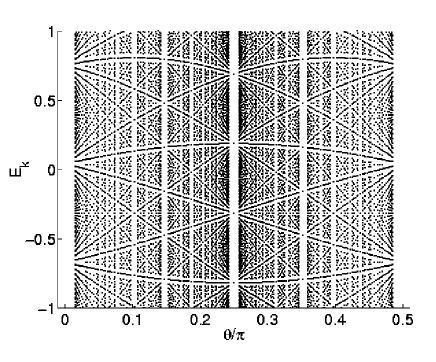
Figure 2: Position of the ground WB-band repeated by the subband energy interval $2\pi F(r^{2}+q^{2})^{-1/2}$ as a function of the field direction $\theta=\arctan(r/q)$ (parameters $\hbar=2$, $F=0.08\sqrt{2}$, $\epsilon=0$, integers $q,r\leq 21$).

It was shown in the previous section that for rational directions of the field the ground WB-subbands repeat with energy splitting $aF/s$. As an example, Fig. 2 shows the relative positions of these subbands as a function of the angle $\theta=\arctan(r/q)$ for $\hbar=2$ and $F=0.08\sqrt{2}$. We recall that in the considered case of a separable potential the bands have zero width for any $\theta\neq 0,\pi/2$.

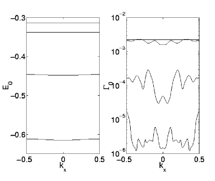
Figure 3: Real (left) and imaginary (right) parts of the dispersion relation ${\cal E}_{\beta}(k_{x},k_{y})$ for the ground WB-states and different values of the potential parameter $\epsilon=0$, $0.1$,$0.5$, and $1$ (from top to bottom). The system parameters are $\hbar=2$, $F_{x}=F_{y}=0.08$, and $k_{y}=0$.

The main difference between separable and non-separable potentials is that the subbands $E^{(i)}_{0}({\bf k})$ have a finite width in the latter case. This is illustrated by Fig. 3(a) which shows the dispersion relation $E_{0}(k_{x},k_{y}=0)$ for the potential (2) with (from top to bottom) $\epsilon=0$, $0.1$, $0.5$, and $1$. The direction of the field is $\theta=\pi/4$, i.e. $r=q=1$. The amplitude of the static field and the value of the scaled Planck constant are the same as in Fig. 2. It is seen in Fig. 3(a) that the WB-bands gain a finite width as $\epsilon$ is increased. We also calculated the dispersion relation $E_{0}(k_{x},k_{y}=0)$ for different angles $\theta=\arctan(r/q)$, with $r,q\leq 6$. It was found that the band widths $\Delta E_{0}=\Delta E_{0}(r,q)$ are typically much smaller than the mean energy separation between the subbands. Thus, for practical purpose, one can neglect the band width for the real part of the spectrum. (An exception is the case $\theta=0,\pi/2$ where the width of the WB-bands approximately coincides with the width of the Bloch band in the absence of the static field.) Neglecting the width of the bands they were found to form a structure similar to that shown in Fig. 2.

We proceed with the analysis of the decay rate of the WB-states, which is determined by the imaginary part of the complex energy, $\Gamma_{0}=-2{\rm Im}({\cal E}_{0})$. In the case of a separable potential the dependence $\Gamma_{0}=\Gamma_{0}(F,\theta)$ is obviously given by the equation

$$\Gamma_{0}(F,\theta)=\Gamma^{\prime}_{0}(F\cos\theta)+\Gamma^{\prime}_{0}(F\sin\theta)\;,$$ (15)

where $\Gamma^{\prime}_{0}(F^{\prime})$ stands for the width of 1D WS-resonances. For the parameters used ($\hbar=2$ and $F=0.08\sqrt{2}$) the dependence (15) is shown in Fig. 4 by a solid line. The maximum around $\theta=\pi/2$ originates from a peak-like behavior of $\Gamma^{\prime}_{0}(F^{\prime})$ and is explained by the phenomenon of 1D resonant tunneling JOB2 .

For a non-separable potential and rational direction of the field the decay rate depends on the quasimomentum. For the particular case $\theta=\pi/4$ this dependence is depicted in Fig. 3(b). We would like to note the complicated behavior of $\Gamma_{0}({\bf k})$. The oscillating character of the decay rate is an open problem for the present day. Because the decay rate depends on the quasimomentum it might be convenient to introduce the notion of $\bar{\Gamma}_{0}$, where the average is taken over the reduced Brillouin zone. The dots in Fig. 4 show the values of $\bar{\Gamma}_{0}$ for some rational direction of the field and two different values of $\epsilon$. It is seen that for a small $\epsilon=0.1$ the ratio $\Delta\Gamma_{0}/\bar{\Gamma}_{0}$ is small and the obtained dependence $\bar{\Gamma}_{0}=\bar{\Gamma}_{0}(r,q)$ essentially reproduces that of the separable case. However, this is not valid for $\epsilon=1$, where the decay rate varies wildly. Thus, in the case of strong coupling between two degrees of freedom the description of WS-state by a mean decay rate is insufficient.

IV Conclusion

We studied Wannier resonances in a 2D system, mainly discussing the complex energy spectrum of the Wannier-Bloch states. However, because the latter are related to the Wannier-Stark states by a Fourier transformation, the obtained results can be easily reformulated in terms of the Wannier-Stark resonances. Then the following is valid. (i) Neglecting the asymptotic tail, WS-states are localized functions along the direction of the field. (This follows from the degeneracy of WB-bands along the field direction.) (ii) For any rational direction of the field [see Eq. (5)] WS-states are Bloch waves in the transverse direction. (iii) For a non-separable potential the corresponding energy bands have a finite width. (iv) For the real part of the spectrum, the band widths are small and can be well neglected for $r,q>1$.

We also found a nontrivial dependence of the resonance width (inverse lifetime of WS-states) on the direction of the field. Because the value of the resonance width defines the decay of the probability, a complicated behavior of the survival probability is expected when the direction of the field is varied. The detailed study of the probability dynamics is reserved for future publication.

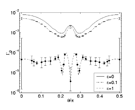
Figure 4: Decay rate of the ground WB-states as a function of the field direction $\theta$ in the case of separable potential ($\epsilon=0$, solid curve). The dashed and dashed-dotted lines are an interpolation to arbitrary $\theta$ of the mean decay rate calculated for some rational directions of the field (dots) for $\epsilon=0.1$ and $\epsilon=1$, respectively. The maximum and minimum values of the decay rate for these angles are indicated by the ‘error’ bars.

References

- (1) Also at L. V. Kirensky Institute of Physics, 660036 Krasnoyarsk, Russia.
- (2) F. Bloch, Z. Phys. 52, (1929) 555; G. Zener, Proc. R. Soc. London, Ser. A 137, 523 (1934); L. D. Landau, Phys. Z. Sov. 1, 46 (1932); G. H. Wannier, Phys. Rev. 117, 432 (1960); A. Rabinovitch and J. Zak, Phys. Rev. B 4, 2358 (1971).
- (3) E. E. Mendez, F. Agullo-Rueda, and J. M. Hong, Phys. Rev. Lett. 60, 2426 (1988); E. E. Mendez and G. Bastard, Phys. Today 46, 34 (1993).
- (4) M. Raizen, C. Solomon, Qian Niu, Physics Today, July 1997, p.30.
- (5) M. Glück, A. R. Kolovsky, H. J. Korsch and F. Zimmer (unpublished)
- (6) M. Glück, A. R. Kolovsky, H. J. Korsch, Phys. Rev. Lett. 83, 891 (1999); Phys. Rev. A 61, 061402(R) (2000); J. Opt. B: Quantum Semiclass. Opt. 2, 612 (2000).
- (7) M. Glück, A. R. Kolovsky, H. J. Korsch, Phys. Rev. Lett. 82, 1534 (1999); Phys. Rev. E 60, 247 (1999).
- (8) M. Glück, A. R. Kolovsky, H. J. Korsch, J. Opt. B: Quantum Semiclass. Opt. 2, 694 (2000).
- (9) In the tight-binding approximation the evolution operator and its eigenfunctions were considered by Q. Niu, PRB 40, 3625 (1989).
- (10) Through the paper we use dimensionless variables where the amplitude of the static field and the scaled Planck constant are the independent parameters of the system. Alternatively, one can set and introduce the notion of the scaled amplitude for the potential (2).
- (11) X.-G. Zhao, R. Jahnke, and Q. Niu, Phys. Lett. A 202, 297 (1995).
- (12) M. Ya. Azbel, Zh. Eks. Teor. Fiz. 46, 929 (1964) [Sov. Phys. ZETP 19, 634 (1964)]; D. R. Hofstadter, PRB 14, 2239 (1976).