The decay of plane wave pulses with complex structure in a nonlinear dissipative medium
Abstract
Nonlinear plane acoustic waves propagating through a fluid are studied using Burgers’ equation with finite viscosity. The evolution of a simple N-pulse with regular and random initial amplitude and of pulses with monochromatic and noise carrier is considered. In the latter case the initial pulses are characterized by two length scales. The length scale of the modulation function is much greater than the period or the length scale of the carrier. With increasing time the initial pulses are deformed and shocks appear. The finite viscosity leads to a finite shock width, which does not depend on the fine structure of the initial pulse and is fully determined by the shock position in the zero viscosity limit. The other effect of nonzero viscosity is the shift of the shock position from the position at zero viscosity. This shift, as well as the linear time, at which the nonlinear stage of evolution changes to the linear stage, depends on the fine structure of the initial pulse. It is also shown that the nonlinearity of the medium leads to generation of a nonzero mean field from an initial random field with zero mean value. The relative fluctuation of the field is investigated both at the nonlinear and the linear stage.
| Radiophysics Dept., University of Nizhny Novgorod | |
| 23, Gagarin Ave., Nizhny Novgorod 603600, RUSSIA | |
| e-mail: gurb@rf.unn.runnet.ru | |
| Department of Mechanics, | |
| Royal Institute of Technology, | |
| S–100 44 Stockholm, SWEDEN | |
| e-mail: benflo@mech.kth.se, | |
| phone: Int+46 8 7907156, fax: Int+46 8 7969850 |
1 Introduction
The propagation of finite amplitude sound waves is of fundamental interest in nonlinear acoustics. In the simplest model of propagation in fluids these waves are described by the well-known Burgers’ equation (plane waves) [1, 2] or modifications of Burgers’ equation, which are called generalized Burgers’ equations (cylindrical and spherical waves) [3, 4, 5]. In studies of nonlinear wave propagation an important problem is to find the waveform of the asymptotic wave at long time after the preparation of the initial wave or at long distance from the source emitting the wave. In the first case the asymptotic wave is called the old-age wave and is an asymptotic solution of an initial value problem of some wave equation and in the latter case the asymptotic wave is a solution of a boundary wave problem. The asymptotic wave is damped both by absorption and by shock wave dissipation and the asymptotic wave is therefore, for plane waves, described by the linear diffusion equation. Because the linear diffusion equation describes the attenuation of high frequency waves, the asymptotic behaviour is determined by the spectrum of the waves of low frequencies. This spectrum is the result of the distortion of the wave at the nonlinear stage.
The decay of a wave to the old-age waveform is very different for periodic signals and pulse perturbations. For the periodic signal the old-age waveform is an exponentially decaying harmonic wave. The pulse perturbation has continuous spectrum and the amplitude of the pulse decays according to a power law.
For sinusoidal and N-wave initial perturbations the old-age solutions have been studied in several papers for plane, cylindrical and spherical waves with use of both analytical and numerical methods [6, 7, 8, 9, 10, 11, 12, 13, 14, 15]. The dependence of the amplitude constant of the old-age waveform on the parameters of the initial perturbations has been found.
The aim of the present paper is to investigate the asymptotic behaviour of complex pulses, such as modulated or random waves. Plane waves are studied, which means that we will use the original form of Burgers’ equation [1]. Burgers’ equation has an exact solution, which is found by reducing it to the linear diffusion equation by mean of the Hopf-Cole transformation [16, 17]. Because of the existence of an exact solution it is relatively easy to find the old-age waveform developing from simple initial perturbations like periodic signals and N-waves in the plane wave case. However, for signals with complex structure it is far from trivial to find their evolution even for plane waves [18, 19, 20]. For a regular signal with fractal structure [18, 20] an unusual sequence of stages of evolution may appear: the nonlinear stage may succeed the linear stage. At the nonlinear stage this wave may decrease more slowly than a periodic wave or a simple pulse.
Still more complicated behaviour is shown by a random signal. The solution of Burgers’ equation with random initial conditions is often called Burgers turbulence. Numerous papers are devoted to investigations of this problem [22, 23, 24, 25, 26, 27]. In the case of vanishing viscosity the continuous random initial field is transformed into a sequence of straight lines with some slope and with random locations of the shocks separating them. Due to the merging of the shocks the internal scale of the turbulence increases and the random wave decreases more slowly than the periodic signal. The decay rate depends on the behaviour of the initial energy spectrum of low frequency [21, 26] and is also sensitive to the statistics of the potential of the initial velocity field [22, 26, 27]. The asymptotic behaviour of the field in the case of finite viscosity also depends strongly on the statistical properties of the initial field. In the case where there are large scale components in the initial spectrum the nonlinear stage never transforms to the linear regime of evolution [21]. In the opposite case the final evolution depends on the tail of the initial probability distribution [23].
In the present paper we consider the evolution of complex pulses which are characterized by two scales: - the inner scale of the carrier, - the scale of the modulation, and the condition . For such signals the generation of a low-frequency component or a non-zero mean field takes place. The case of vanishing viscosity has been investigated [29, 31]. It has been shown that, after multiple merging of the shocks, the inner structure disappears and finally a finite pulse ends up with an N-wave. This N-wave is fully described by the positions of its zero and shocks, which are determined by the potential of the initial velocity : . It has also been shown that, for a pulse with random carrier, the fluctuations of the positions of the zero and the shocks are relatively small for .
In the present paper we will consider the influence of finite viscosity on the nonlinear stage of the evolution of the pulse and investigate its old-age behaviour. The paper is organized as follows.
In section 2, on the base of the Hopf-Cole solution, the asymptotic behaviour of the pulse at the nonlinear and the old-age stages is analyzed in general terms without assuming the detailed structure of the initial pulse.
In section 3 the evolution of simple N-waves with regular and random amplitude is discussed.
Section 4 deals with pulses with monochromatic carrier and section 5 with pulses with noise carrier. It is shown that the parameters of the asymptotic waveform depend weakly on the fine structure of the initial pulse, but that the old-age behaviour is very sensitive to the properties of the carrier.
2 Solution of Burgers’ equation and its large time asymptotics
Our starting-point is the Burgers’ equation
| (1) |
which governs the propagation of plane acoustic waves in nonlinear dissipative media. Here is the velocity of fluid and is the fluid viscosity. Burgers’ equation (1) has the Hopf-Cole solution [16, 17]
| (2) |
where is the solution for the linear diffusion equation
| (3) |
Here is the Green function of the linear diffusion equation
| (4) |
and is the initial condition for this equation
| (5) |
which corresponds to the initial condition
| (6) |
The main goal of the present paper is the investigation of the old-age behaviour of the localized pulses. But first we discuss shortly the asymptotic evolution of nonlocalized waves. Consider a group of perturbation with the bounded initial potential assuming that is a periodic signal with a period or homogeneous noise with rather fast decreasing probability distribution of the potential . For such a perturbation in (3) we separate a constant component :
| (7) |
Inserting (7) into (3) we see that does not depend on time, since the -integral of is unity. Here is a field with zero mean value (on the period or statistically for noise). As times goes on, the viscous dissipation and oscillation (inhomogenity) smoothing causes the amplitude (variance) of the field to become less. At times when it amounts to the solution (2) is equal to
| (8) |
As satisfies the linear diffusion equation, then also at these times fulfils the linear equation. This testifies precisely to the fact that the evolution of the velocity field enters the linear stage. The accumulated nonlinear effects are described in this solution by the nonlinear integral relation between the initial velocity field and the fields , (5,6), and are characterized by the value .
Here is the characteristic change in amplitude of , and is the initial Reynolds number.
From (8) it is easy to get the well known result, that for the initial harmonic waves asymptotically has also harmonics form, but with the amplitude not depending on the initial amplitude [2, 3].
At large initial Reynolds number the homogeneous Gaussian field at the nonlinear stage transforms into series of sawtooth waves with strong nongaussian statistical properties [21, 25]. Nevertheless at very large time, when the relation (8) is valid, the distribution of the random field with statistically homogeneous initial potential converges weakly to the distribution of the homogeneous Gaussian random field with zero mean value, and universal covariance function [23]. But the amplitude of this function is nonlinearly related to the initial covariance function of the field and increases proportionally with increasing of initial Reynolds number [21, 23].
Let us consider the opposite situation when the initial perturbation is localized in some region. We assume also that initial potential vanishes very fast for , so we have
| (9) |
where can be considered as the length of initial pulse. The condition (9) is identical to the assumption that the integral over the initial pulse is zero.
It should be stressed that if the integral over the initial pulse is , then the initial perturbation transforms to the unipolar pulse with area asymptotically. For the form of this pulse is close to the triangular with the width of shock much smaller than the length of the pulse . For such a pulse and does not depend on time. Thus the nonlinear stage of the evolution prevails for all times.
Let us now consider the time asymptotic behaviour of initially localized pulse which satisfies (9). If we rewrite (3) as
| (10) |
then we can see that because of (9) the integrand at right hand side of (10) is zero outside the region . It is seen from (4) that the length scale of Green’s function is
| (11) |
If the length scale of is called , and the following condition
| (12) |
is valid, then Green’s function can be considered as constant in the interval where the integrand at the right hand side of (10) is significantly different from zero. Thus we obtain from (10) using (5)
| (13) |
Here , , is the value of , in the neighborhood of which the integrand in (10) gives the essential contribution in the integral. In (13) we introduce the notation
| (14) |
We assume . From (3),(13),(14) an approximate solution is obtained
| (15) |
If the initial pulse is centered around , and the large scale of the field is much greater then , then we can put and obtain
| (16) |
instead of (15). For large initial Reynolds number , where is the maximum of , the constant (14) may be rewritten as the product of the maximum of the integrand and some length:
| (17) |
Using the definition of Green’s function (4) and (17) we can rewrite (16) in the form
| (18) |
In the limit of vanishing viscosity () we get from (18) the well known solution for N-wave
| (19) |
where is the position of the shock
| (20) |
At this stage the form and the energy of the pulse
| (21) |
are determined only by the value of maximum of initial potential and does not depend on the fine structure of the pulse. This limiting case () for the pulses with complex inner structure was investigated in the paper [31].
For large but finite Reynolds number the solution (18), completed with a solution valid at near and exhibiting the shock structure, is valid only at finite time. For finite values and sufficiently small we still have
| (22) |
Then for
| (23) |
| (24) |
we obtain the increasing part (in ) of the N-wave solution (19). On the other hand, for , fixed, we find that fades away exponentionally.
For , arbitrary finite, we have
| (25) |
and the solution (16) can be approximated as
| (26) |
Using (4) we can rewrite the condition of the validity of the solution (26) as
| (27) |
Because (24) gives a solution of the linear diffusion equation, the condition (27) defines the linear stage of the pulse evolution. On this stage the pulse energy is
| (28) |
Thus at the linear stage of evolution of the pulse has a universal form (26) and is determined only by the constant , which is defined by the initial perturbation by the relation (14). The case can be understood by comparing the definition of according to the equations (14) and (5) with the formulas (30) - (33) in ref. [19]. By this comparison it is clearthat the case corresponds to the absence of the Fourier component with in the terminology of ref. [19]. The Fourier component with is absent here already for . The case excludes the N-wave solution (19).
Below we will consider three cases of initial perturbation, assuming that the initial potential may be written in the form
| (29) |
where has the scale . First we consider the simplest case when is constant, either deterministic or random value. Here we discuss the main properties of the wellknown solution (see ref. [30]) for the N-wave. The cases of monochromatic and noise carrier will be considered in Sections 4 and 5. In these cases we assume that the scale of the carrier satisfies the condition and then
| (30) |
3 The decay of a simple pulse with random initial amplitude
3.1 The evolution of a regular N-wave
We discuss the evolution of a one scale pulse, whose potential has the structure in (29):
| (31) |
Here is a constant and is a dimensionless function with the scale :
| (32) |
In particular we will consider the cases where the initial perturbation (31), (32) is exact in the interval and outside this interval. We first assume and find from (6) that the initial velocity pulse is an N-wave:
| (33) |
From (5) we then obtain
| (34) |
From (34) we find that for this special case the length scale of , first introduced in (11), is (the square root of the inverted coefficient of in (34))
| (35) |
The calculation of , from which we obtain by use of (2), can now be done using (10) with insertion of (34) and (4):
| (36) |
The definition of the error function is:
| (37) |
The asymptotic behavior of the error function for large arguments is
| (38) |
Using (38) we find from (36) for , finite, :
| (39) |
On the other hand, for we have for finite and , and (the last inequality is necessary for the cancellation of the last two error functions in (36)):
| (40) |
For , finite and we can neglect the second term at the righthand side of (40). Taking with finite in (39) or (40) we obtain using (2):
| (41) |
where is the shock coordinate
| (42) |
However, for growing -values the sharp discontinuity of the N-wave solution (41) is broadened and we can calculate a shockwidth which depends on a small but finite value of . Using (40) in (2) and assuming that
| (43) |
we obtain
| (44) |
Using (14) and (32) we find for the present case in (17) and
| (45) |
and thus, using (4), we see that the result (44) is a special case of (16).
From the expression (44) we will now find the width of the shock. If we define the position of the shock as the coordinate where the wave amplitude has decreased to half its maximal value, we find from (23) the following expression for :
| (46) |
Evaluating the expression (44) for in the neighborhood of the shock, or more precisely, for
| (47) |
we find
| (48) |
where the shockwidth is given as
| (49) |
In order to decide which of the two waveforms (41) and (48) is most appropriate we compare the expressions for (42) and (46). From these formulas we see directly that the shock velocity () decreases faster for growing with nonzero viscosity. The zero viscosity expression (42) can be used as long as the correction to the N-wave shock position is much greater in (42) than in (46), which means
| (50) |
where the nonlinear time is defined as
| (51) |
In the notation , stands for the kind of pulse and stands for ”nonlinear”.
The energy of a pulse is defined as the integral over the pulse length of the square of the fluid velocity. We will calculate the energies of some of the pulses studied above. For the N-wave (41) we obtain
| (52) |
Thus for and (50) still valid we see from (52) that behaves like (21) and thus depends on the initial scale only in the next order of , i.e. .
The energy of the wave under the condition but (50) no longer valid is obtained from (44). We obtain
| (53) |
After transformation of the integral in (53) we obtain
| (54) |
where is given in (45). We need the formula ([32], formula (2.3.13.27))
| (55) |
where is given by the power series
| (56) |
Using (55), with and , in (54) an energy expression, valid for and (cf. (50)) , is obtained:
| (57) |
From (57) the energy of the wave in the linear region is obtained by keeping only the power zero in the series for :
| (58) |
which is a special case of (28) with given by (45). After introduction of the ”linear” time , the validity condition of (58) is written:
| (59) |
For the negative the pulse decays much faster than for . For at the initial pulse transforms into so called S-wave [2, 31], and the energy becomes
| (60) |
which is independent of the initial amplitude of the pulse. Of course the reason why the energy of the S-wave decreases faster with than the energy of the N-wave is that the length of the N-wave increases with growing in contrast to the S-wave.
At large Reynolds number the constant (14) which determines the linear stage of evolution is
| (61) |
and much smaller than for positive with the same Reynolds number. The region of validity of linear regime is obtained from (25) and (61) as
| (62) |
Thus for the pulses with negative the linear stage begins much earlier than for the pulses with positive , for which the linear time (59) increases exponentionally with the Reynolds number .
Nevertheless, we can see on this simple example the main nontrivial properties of the old-age behavior of the pulses in the case of large Reynolds number.
In the limit of vanishing viscosity () the energy of the pulse (21),(52) and the shape of the pulse (19),(20),(41) do not depend on the length of asymptotically for . They are determined only by the maximum of initial potential (in our case – of the area of triangular pulse of initial pulse ). Nevertheless, at the linear stage the energy depends not only of , but is also proportional to (53). We can remark that the energy of initial pulse is proportional to .
The other property that we stress is that the amplitude (17),(45) of the wave at the old-age stage depends exponentially on the amplitude of the initial pulse. For small wave numbers the Fourier component of the pulse depends linearly on : . At the linear stage the slope of the Fourier component does not depend on time: . At the nonlinear stage the growing of the slope until the very large linear time (59) leads to an exponentionally large value (in ) of at the linear stage (cf.(45)).
3.2 The decay of an N-wave with random amplitude
Let us discuss the evolution of N-wave (33) with random initial amplitude. We assume that the amplitude in (31) has a gaussian probability distribution function with a zero mean value
| (63) |
From (33) it is easy to see that mean initial field is zero, and relative fluctuation of the energy (52) at is
| (64) |
In the previous section it was shown that there is strong difference between the decay of the pulse with positive and negative amplitude . If we introduce – the mean energy of pulse with positive amplitude (N-wave), and – the mean energy of pulse with negative amplitude (S-wave), then at time
| (65) |
from (52), (60) and (63) we have
| (66) |
This fast decrease of pulses with negative will lead to the generation of a field with positive mean value from an initial field with zero mean value .
At time (65) we can neglect the influence of the negative pulse on the mean field and use the expressions (19),(20) for the velocity. In different realizations we will have the N-wave with the same slope and random position of the shocks.
Let us introduce the cumulative probability of the random amplitude
| (67) |
| (68) |
From (68) we obtain for the mean velocity and its variance the following expressions:
| (69) |
| (70) |
For the Gaussian distribution of (63) we have from (67), (69)
| (71) |
| (72) |
where is the error function (37).
At small the mean field is half the regular field with , due to the fact that only in that half of realizations, in which , we have a relatively slowly decaying N-wave. The mean field (71) has not a clear stressed shock front and has a very fast decaying tail at :
| (73) |
It is easy to see that both mean field and variance have self-similar behaviour
| (74) |
where , are given as:
| (75) |
Due to the self-similarity the relative integral fluctuation of the field
| (76) |
does not depend on and is of the order of unity.
The situation radically changes on the linear stage when the field is described by the equation (26). At this stage we have the self-similar evolution of the field
| (77) |
where is defined as
| (78) |
and is a random amplitude (45) with nonzero mean value. For the gaussian distribution of in (29) we have from (14)
| (79) |
Here we introduce the effective Reynolds number
| (80) |
From (79) we see that mean value does not depend on the fine structure of the carrier and is always positive. The positive mean value is a result of generation of mean field at the nonlinear stage. Here we consider the case of large Reynolds number, where we can use the asymptotic expression for (45). The n-th moment of will be expressed through the probability distribution function (p.d.f.) of (63):
| (81) |
Using the steepest descent method for we have from (63), (81)
| (82) |
Thus we have very fast growing of the momentum with increasing . From (77) one can see that at the linear stage both mean field and variance are self-similar, and that the relative integral fluctuation does not depend on . But in contrast to the nonlinear stage (76), in the linear stage the relative integral fluctuation of the field is extremely large for large Reynolds number:
| (83) |
We have similar behaviour also for the relative fluctuation of the energy (64). At the nonlinear stage at we have from (21), (63), (64)
| (84) |
Thus at the nonlinear stage does not depend on the initial scale and the variance of the p.d.f. of amplitude .
4 The evolution of a pulse with monochromatic carrier
In this section we consider the evolution of a pulse with monochromatic carrier
| (86) |
Here , and we assume that the length scale of the modulation function is much greater then the period of the carrier (). Below we consider two large parameters and . For different ratios of these parameters we have different regimes of wave evolution.
The pure monochromatic signal is characterized by the nonlinear time (”” stands for ”signal”) and the linear time [21]. At () the monochromatic wave transforms into the sawtooth wave with the slope . The shock amplitude , as well as the energy of the wave , does not depend on the initial amplitude. The shockwidth
| (87) |
increases with time, and is, at , of the same order as a period. For we have the linear regime of evolution, where the wave form is sinusoidal again with exponentionally decaying amplitude .
For a pulse with monochromatic carrier a large-scale component is generated. The interaction of the high frequency component with the large-scale wave will change the evolution of the carrier.
4.1 The nonlinear stage of evolution at large Reynolds number
Below we give a short summary of pulse evolution at based on the paper [31], and discuss the influence of finite dissipation on the evolution of large scale and high frequency carrier.
The nonlinear effect leads to the generation of the large-scale component , and at this component obtains the stationary form
| (88) |
which is equal to the form of simple pulse with the same initial potential . The evolution of the large-scale component is characterized by the nonlinear time (51), and (88) is valid for . At time
| (89) |
the energy of large-scale and small-scale components are of the same order. At the evolution of the large-scale component is equal to the evolution of a simple pulse with .
For the evolution of the large-scale component is described by the expressions (41), (42), (52). At , in the limit , the evolution of the large-scale component is determined by only one parameter of the initial perturbation.
At the amplitudes of the shocks of the small-scale components do not depend on the initial amplitude: , but due to the interaction with large-scale component they have nonzero velocity (88), where is the initial position of the shock. The distance between the shocks increases with time as
| (90) |
The collision of the shocks of small-scale components moving with constant velocity of fine structure with shocks of the large-scale structure (42) leads to decrease of the number of shocks (see fig. 3 from [31]). The last collision occurs at time , and after this time a pure N-wave remains.
At finite Reynolds number the width of the shocks of the large-scale component increases with time (87). The linear spreading of small structure leads to the increase of the distance between the shocks (90). Comparing (87) with (90) we find that, if the initial Reynolds number satisfies the condition
| (91) |
then the nonlinear structure of shocks will be conserved. This is because the relative shock width is
| (92) |
In the opposite case, under the condition
| (93) |
the nonlinear structure will dissipate before the nonlinear distortion of large-scale component begins.
The evolution of the large-scale component at finite Reynolds number will be described by the same equations as the evolution of a simple wave (47) - (49). Only the position of the shocks will be determined by some other equation (23), where depends on the fine structure of the initial pulse. This dependence leads to the sensitivity of the old-age behaviour on the fine structure of the initial pulse.
4.2 Old-age linear stage evolution of pulse with monochromatic carrier
The final linear stage of evolution is described by the equation (26), where the constant (14) is now given by
| (94) |
At large Reynolds number the constant may be written in the form (17). In fact for the large Reynolds number the main contribution in the integral in (94) comes from the neighborhood of points . An evaluation of by the steepest descent method then gives
| (95) |
From (95) we see that the prefactor in (17) strongly depends on the ratio of two large numbers: the Reynolds number and the number . When the relation (91) is valid, then only the first term in (95) is significant, and from (17), (95) we have
| (96) |
In the case of moderate Reynolds number, when the condition (93) is valid, we have from (17,95)
| (97) |
The results above should be compared with expression (45) of for the simple pulse for which we have . One can see that the modulation leads to faster transformation of the wave into the linear regime of evolution and consequently to decrease of the amplitude of the wave () at the old-age stage.
5 The evolution of a pulse with noise carrier
In this section we will study the evolution of a pulse with noise carrier (30). We assume that the potential is homogeneous gaussian noise with rapidly decreasing covariance function
| (98) |
In the limit of vanishing viscosity the continuous homogeneous field transforms into sequence of sawtooth pulses with equal slope and with random position of shocks. Due to the collision and merging of the shocks, their number decreases and the characteristic scale of random field increases. This effect makes all the statistical properties of the field self-similar and they are determined by only one scale , which can be interpreted as characteristic distance between the zeroes of or between the shocks [21, 25, 26].
The evolution of the integral scale in time due to merging of the shocks ([21], see eq. 4.15, p. 170)
| (99) |
depends on only two integral characteristics of the initial homogeneous field
| (100) |
Here is the correlation length of the initial potential. Due to the merging of the shocks the energy density of the random wave decreases slower then the energy of harmonic perturbation.
In case of the finite Reynolds number the thickness of the shock in the sawtooth wave originating from a monochromatic wave is given in (87). We have the same expression for a random wave as well, where is the random amplitude of the shock. For the estimations we can assume .
The ratio between the integral scale and internal scale is the effective Reynolds number :
| (101) |
where and (”” stands for ”noise”) are defined as
| (102) |
Thus the effective Reynolds number logarithmically slowly decreases with time, and the linear stage of evolution starts at very large time , . At this time the nonlinear effects become unimportant and the noise enters into the linear mode where its damping is mainly determined by linear dissipation. On the base of the solution (8), as it was shown in [21], the energy decays as
| (103) |
At the linear stage the distribution of the random field converges to the distribution of the homogeneous Gaussian field with zero mean velocity and variance according to (103) [23].
The evolution of the pulse with noise carrier in the limit of vanishing viscosity was considered in the paper [31]. It was shown that an initial perturbation transforms to an N-wave. In the case, when the scale of the carrier is much smaller then scale of modulation function , it was shown that the fluctuation of the shock positions is relatively small.
Below we consider the properties of the pulse with noise carrier at the nonlinear stage for finite Reynolds number and the old-age behaviour of the pulse.
5.1 Nonlinear stage of evolution of pulse with noise carrier
In the case of vanishing viscosity we can introduce two characteristic times: the nonlinear time for noise carrier evolution and nonlinear time for modulation evolution . At the initial wave transforms into the sequence of sawtooth pulses, with the integral scale and the energy density depending slowly on the coordinate [31]. At this stage the nonlinearity leads to partial depression of modulation and to generation of the mean field [31]. Due to the merging of the shocks their number decrease, and at the initial pulse with noise carrier transforms into an N-wave with random positions of zero and shocks. The position of the N-wave zero is localized in an narrow region near the center of the initial pulse [31]. The position of the shocks are determined by the equation (20), where is the value of absolute maximum of the initial potential (29). It was shown that the cumulated probability has the form [31]
| (104) |
Here is the mean number of intersections of level by the initial potential in the interval (9), is a characteristic scale of the modulation function (32) , is an integral scale of the Gaussian homogeneous carrier potential and is its variance (100).
The mean velocity , with given by (68) and its variance are described by equations (69), (70), where now the cumulative probability is determined by equation (104), and not by the error function in (71). It is easy to see from (74) that both mean field and variance have self-similar behaviour. From (69) , (70), (104) we have (cf. (74))
| (105) |
| (106) |
where , and is a large parameter, proportional to the number of correlation lengths on the whole extension of the pulse:
| (107) |
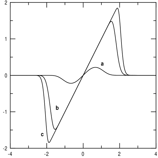
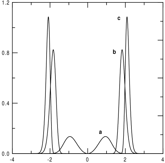
Contrary to the case of the simple initial pulse (75), in the case of pulse with noise carrier the mean field and its variance have two different scales for (see figs. 1 and 2). The two scales in the ”b” and ”c” curves in the figures are the width of the shock and the length of the pulse. In the ”a” curves only the length of the pulse remains. For the function at . The function increases rather fast to in the narrow region .
Thus for the mean field has the N-wave similar structure with the dimensionless shock position
| (108) |
The relative width of the shock of the mean field is
| (109) |
In the neighborhood of the shock position we can introduce a new variable z:
| (110) |
and from (106) we see that the shape of the front is described by double exponential distribution
| (111) |
The variance is different from zero in a narrow region (109) near the shock position and for the relative integral fluctuation of the field (76) we have from (105), (106)
| (112) |
A finite Reynolds number leads to a finite width of the shock. The shock structure in each realization is described by the expressions (48), (49). The shifting of the shock position from the zero viscosity limit is given in (23). At the nonlinear stage we can neglect this shifting. Then in each realization we have self-similar evolution of the pulse, and the relative width of the shock does not depend on time. While for () the maximum of the initial potential is localized in the narrow region near ([31] formulas (107), (113)), we can estimate the relative width of shock front as
| (113) |
Comparing (113) with (109) we see that the influence of finite viscosity on the mean field is unimportant if
| (114) |
In the opposite case, for extremely large ratio , the width of the mean field will be determined by the viscosity.
The displacements of shock position (23) from the vanishing viscosity position leads finally to the depressing of nonlinear effects. For (cf.(27)) we have the linear stage of evolution. While for the random perturbation we have a large fluctuation of , the cumulative action of nonlinearity, which is proportional to , leads to strong fluctuation of the field at the linear stage.
5.2 Old-age linear stage of evolution of a pulse with noise carrier
At the old-age stage, when the evolution of the pulse is described by linear solution (26) all the properties of the wave are determined by the constant , given in (14). The potential (29) is a random Gaussian function. The mean value of is given by the equation (79), and does not depend on the fine structure of the carrier. For we have from (82)
| (115) |
Let us first consider the case of relatively large Reynolds number, when the integral (14) may be calculated using the steepest descent method, and only the contribution of the absolute maximum is important:
| (116) |
Here is the value of absolute maximum of , and is the second derivative of the potential at this point. To find the statistical properties of we need to know the joint probability distribution of and . From (98) it is easy to find the correlation coefficient for and : . If we consider the conditional probability distribution function , we then obtain for the conditional mean value and variance :
| (117) |
While increases exponentionally with only the maximum gives a significant contribution to the average characteristics of . Thus in (116) we can substitute (117) instead of , and so we have
| (118) |
From (104) we have for the probability distribution function of the absolute maximum of the initial potential :
| (119) |
This function is localized near
| (120) |
and has a tail for :
| (121) |
For the calculation of the moments of we can use the steepest descent method using the tail of the probability distribution function (121):
| (122) |
We have the main contribution for the n-th moment (122) at the point . Comparing with given in (120) we see that the inequality (114) is necessary for (122) to be valid.
Comparing (122) with the relation (82) for the moment of for a simple pulse we see that for the small-scale noise carrier the moments depend on the integral scale of the carrier.
The relative integral fluctuation of the field (76) on this stage is expressed for two first moments of as
| (123) |
and when the condition (114) is valid it is very large in contrast to the nonlinear stage (112), where . For the noise carrier with the scale the relative integral fluctuation is the small factor times the fluctuation of the simple pulse with random Gaussian amplitude (83).
The calculation of may be done directly on the base of the integral (14), and for large Reynolds number we have the same equation (123). For we have relatively small fluctuation of , and with increasing of the probability distribution of approaches slowly the normal distribution (normalization). This normalization is similar to the normalization of the homogeneous field at the old-age stage [23]. But while the moment increases exponentionally with , we have weak convergence to the normal distribution of like in [23].
6 Discussion and conclusion
We have investigated the evolution of pulses with complex structure in nonlinear media, described by Burgers’ equation. The investigation for vanishing viscosity was done in our paper [31]. There it was shown that the asymptotic form of an arbitrary initial pulse with zero area is an N-wave. It was also shown that the shock positions of the N-wave are determined by only one parameter of the initial perturbation - the value of the absolute maximum of the initial potential (). It was also shown in the paper [31] that for the noise carrier the fluctuations of the shock positions are relatively small if the carrier length scale is much smaller than the modulation length scale .
In the present paper we have considered the evolution of pulses with complex structure at large but finite Reynolds number. On the base of the Hopf-Cole solution it is shown that the finite viscosity leads to a finite shock width , which does not depend on the fine structure of the initial pulse and is fully determined by the shock position in the zero viscosity limit. The other effect is the shift of the shock position from the zero viscosity limit position. This shift depends on the fine structure of the initial pulse, and as a consequence the time , at which the nonlinear stage of evolution changes to the linear stage, is determined not only by the value of the maximum of the initial potential but also by the fine structure of the pulse. Because the amplitude of the pulse at the linear old-age stage is determined by the time , the old-age amplitude is also sensitive to the inner structure of the pulse.
In this paper the evolution of a simple N-pulse with regular and random initial amplitude and of pulses with monochromatic and noise carrier is considered. It is shown that the nonlinearity of the medium leads to the generation of a non-zero mean field from an initial random field with zero mean value. It is also shown that, at the nonlinear stage, the relative fluctuation of the field and its energy is of unit order for simple pulses and small for pulses with complex inner structure (). However, at the old-age linear stage this fluctuation increases exponentially with increasing initial Reynolds number.
Acknowledgements
This work was supported by a grant from the Royal Swedish Academy of Sciences, by the grant INTAS No 97-11134 and by the RFBR grant No 99-02- 18354. Sergey Gurbatov thanks the staff of the Department of Mechanics (KTH) and other friends in Sweden for their warm hospitality.
References
- [1] J.M. Burgers: The Nonlinear diffusion equation. D. Reidel, Dordrecht, 1974.
- [2] G.B. Whitham: Linear and nonlinear waves. Wiley, New York, 1974.
- [3] O. Rudenko, S. Soluyan: Theoretical foundations of nonlinear acoustics. Plenum, New-York, 1997.
- [4] D.G. Crighton: Model equations of nonlinear acoustics. J. Fluid Mech. 11 (1979) 11–33.
- [5] P.L. Sachdev: Nonlinear Diffusive Waves: Cambridge University Press 1987.
- [6] D.G. Crighton, J.F. Scott: Asymptotic solutions of model equations in nonlinear acoustics. Phil. Trans. R. Soc. Lond. A292 (1979) 101–134.
- [7] J.F. Scott: Uniform asymptotics for spherical and cylindrical nonlinear acoustic waves generated by a sinusoidal source: Proc. R. Soc. Lond. A375 (1981) 211–230.
- [8] B. O. Enflo: Asymptotic behavior of the N-wave solution of Burgers’ generalized equation for cylindrical acoustic waves: J. Acoust. Soc. Am. 70 (1981) 1421–1423.
- [9] B. O. Enflo: Saturation of a nonlinear cylindrical sound wave generated by a sinusoidal source. J. Acoust. Soc. Am. 77 (1985) 54–60.
- [10] P.L. Sachdev, V.G. Tikekar, K.R.C. Nair: Evolution and decay of spherical and cylindrical N-waves. J. Fluid Mech. 172 (1986) 347–371.
- [11] P.L. Sachdev, K.R.C. Nair: Evolution and decay of spherical and cylindrical acoustic waves generated by a sinusoidal source. J. Fluid Mech. 204 (1989) 389–404.
- [12] P.W. Hammerton, D.G. Crighton: Old-age behaviour of cylindrical and spherical nonlinear waves: numerical and asymptotical results. Proc. R. Soc. Lond. A422 (1989) 387–405.
- [13] B.O. Enflo: Some analytic results on nonlinear acoustic wave propagation in diffusive media. Radiofizika 36 (1993) 665–686.
- [14] B.O. Enflo: Saturation of nonlinear spherical and cylindrical sound waves. J. Acoust. Soc. Am. 99 (1996) 1960–1964.
- [15] B.O. Enflo: On the connection between the asymptotic waveform and the fading tail of an initial N-wave in nonlinear acoustics: Acustica - Acta Acustica 84 (1998) 401–413.
- [16] J.D. Cole: On a quasi-linear parabolic equation occurring in aerodynamics. Quart. Appl. Math. 9 (1951) 225–236.
- [17] E. Hopf: The partial differential equation . Comm. Pure Appl. Mech. 3 (1950) 201–230.
- [18] S.N. Gurbatov, D.B. Crighton: The nonlinear decay of complex signals in dissipative media. Chaos 5(3) (1995) 524–530.
- [19] O. Brander, J. Hedenfalk: A new formulation of the general solution to Burgers’ equation. Wave Motion 28 (1998) 319–332.
- [20] J.R. Angilella, J.C. Vassilicos, Spectral, diffusive and spiral fields, Physica D (1998), in press.
- [21] S.N. Gurbatov, A.N. Malakhov, A.I. Saichev: Nonlinear random waves and turbulence in nondispersive media: waves, rays, particles. Manchester University Press, Manchester, 1991.
- [22] S.E. Esipov: Energy decay in Burgers turbulence and interface growth : the problem of random initial conditions II: Phys. Rev. E 49 (1994) 2070–2081.
- [23] S. Albeverio, A.A. Molchanov, D. Surgailis: Stratified structure of the universe and Burgers’ equation – a probabilistic approach. Prob. Theory Relat. Fields 100 (1994) 457–484.
- [24] J.P. Bouchaud, M. Mézard, G. Parisi: Scaling and intermittency in Burgers turbulence. Phys. Rev. E 52 (1995) 3656–3674.
- [25] S.A. Molchanov, D. Surgailis, W.A. Woyczynski: Hyperbolic asymptotics in Burgers’ turbulence and extremal processes. Comm. Math. Phys. 168 (1995) 209–226.
- [26] S.N. Gurbatov, S.I. Simdyankin, E. Aurell, U. Frisch, G. Toth: On the decay of Burgers turbulence. J. Fluid Mech, 344 (1997) 339–374.
- [27] G.M. Molchan: Burgers equation with self-similar Gaussian initial data: tail probabilities. J. of Stat. Phys. 88 (1997) 1139–1150.
- [28] J.P. Bouchaud, M. Mézard, Universality classes for extreme-value statistics. Journal of Physics A - Mathematical and General 30 (1997) 7997–8015.
- [29] S.N. Gurbatov, I.Y. Demin: Transformation of strong acoustic noise pulses. Akust. Zh. 28(5) (1982) 634-640. [Eng. translation: Sov. Phys. acoustics 28(5) 375–379.]
- [30] P.L. Sachdev, K.T. Joseph, K.R.C. Nair: Exact N-wave solutions for the non-planar Burgers’ equation. Proc. R. Soc. Lond. A445 (1994) 501-517.
- [31] S.N. Gurbatov, B.O. Enflo, G.V. Pasmanik: The decay of pulses with complex structure according to Burgers’ equation. Acustica - Acta Acustica 85 (1999) 181-196.
- [32] A.P. Prudnikov, Yu.A. Brychkov, O.I. Marichev: Integrals and series, Vol. 1: Elementary functions. Gordon and Breach, Glasgow, 1988.