Measurements of the instantaneous velocity difference and local velocity with a fiber-optic coupler

Abstract

New optical arrangements with two single-mode input fibers and a fiber-optic coupler are devised to measure the instantaneous velocity difference and local velocity. The fibers and the coupler are polarization-preserving to guarantee a high signal-to-noise ratio. When the two input fibers are used to collect the scattered light with the same momentum transfer vector but from two spatially separated regions in a flow, the obtained signals interfere when combined via the fiber-optic coupler. The resultant light received by a photomultiplier tube contains a cross-beat frequency proportional to the velocity difference between the two measuring points. If the two input fibers are used to collect the scattered light from a common scattering region but with two different momentum transfer vectors, the resultant light then contains a self-beat frequency proportional to the local velocity at the measuring point. The experiment shows that both the cross-beat and self-beat signals are large and the standard laser Doppler signal processor can be used to measure the velocity difference and local velocity in real time. The new technique will have various applications in the general area of fluid dynamics.

OCIS codes: 120.7250, 060.2420, 060.1810, 030.7060.

I Introduction

Measurements of the velocity difference or the relative velocity, $\delta{\bf v}({\bf\ell})={\bf v}({\bf x}+{\bf\ell})-{\bf v}({\bf x})$, between two spatial points separated by a distance $\ell$ have important applications in fluid dynamics. For example, in the study of turbulent flows one is interested in the scaling behavior of $\delta{\bf v}(\ell)$ over varying distance $\ell$, when $\ell$ is in the inertial range, in which the kinetic energy cascades at a constant rate without dissipation.[1, 2] If the separation $\ell$ is smaller than the Kolmogorov dissipation length,[1, 2] the measured $\delta{\bf v}(\ell)$ becomes proportional to the velocity gradient $\partial v/\partial r\simeq\delta{\bf v}(\ell)/\ell$ (assuming $\ell$ is known), a useful quantity which is needed to determine the energy dissipation and flow vorticity. In many experimental studies of fluid turbulence, one measures the local velocity as a function of time and then uses Taylor’s frozen turbulence assumption to convert the measured temporal variations into the spatial fluctuations of the velocity field.[3] The frozen turbulence assumption is valid only when the mean velocity becomes much larger than the velocity fluctuations. For isotropic turbulent flows with a small mean velocity, direct measurement of $\delta{\bf v}(\ell)$ is needed.

Over the past several years, the present authors and their collaborators have exploited the technique of homodyne photon correlation spectroscopy (HPCS) to measure $\delta{\bf v}(\ell)$.[4, 5] With the HPCS scheme, small particles seeded in a flowing fluid are used to scatter the incident laser light. The scattered light intensity $I(t)$, which fluctuates because of the motion of the seed particles, contains Doppler beat frequencies of all particle pairs in the scattering volume. For each particle pair separated by a distance $\ell$ (along the beam propagation direction), their beat frequency is $\Delta\omega_{2}={\bf q}\cdot\delta{\bf v}(\ell)$, where $\bf q$ is the momentum transfer vector. The magnitude of $\bf q$ is given by $q=(4\pi n/\lambda)\sin(\theta/2)$, where $\theta$ is the scattering angle, $n$ is the refractive index of the fluid, and $\lambda$ is the wavelength of the incident light. Experimentally, the Doppler beat frequency $\Delta\omega_{2}$ is measured by the intensity auto-correlation function,[6]

$$g(\tau)=\frac{\langle I(t+\tau)I(t)\rangle}{\langle I(t)\rangle^{2}}=1+bG(\tau),$$ (1)

where $b$ ($\leq 1$) is an instrumental constant and henceforth we set $b=1$. The angle brackets represent a time average over $t$.

It has been shown that $G(\tau)$ in Eq. (1) has the form[7]

$$G(\tau)=\int_{0}^{L}dr~{}h(r)\int_{-\infty}^{+\infty}d\delta v~{}P(\delta v,r)\cos(q\delta v\tau),$$ (2)

where $\delta v$ is the component of $\delta{\bf v}$ in the direction of $\bf{q}$, $P(\delta v,r)$ is the probability density function (PDF) of $\delta v(r)$, and $h(r)dr$ is the number fraction of particle pairs with separation $r$ in the scattering volume. Equation (2) states that the light scattered by each pair of particles contributes a phase factor $\cos(q\tau\delta{\bf v})$ (because of the Doppler beat) to the correlation function $G(\tau)$, and $G(\tau)$ is an incoherent sum of these ensemble averaged phase factors over all the particle pairs in the scattering volume. In many previous experiments,[7, 8, 9, 10] the length $L$ of the scattering volume viewed by a photodetector was controlled by the width $S$ of a slit in the collecting optics.

While it is indeed a powerful tool for the study of turbulent flows, the HPCS technique has two limitations in its collecting optics and signal processing. First, a weighted average over $r$ is required for $G(\tau)$ because the photodetector receives light from particle pairs having a range of separations ($0<r<L$). As a result, the measured $G(\tau)$ contains information about $\delta{\bf v}(\ell)$ over various length scales up to $L$. With the single slit arrangement, the range of $L$ which can be varied in the experiment is limited. The lower cut-off for $L$ is controlled by the laser beam radius $\sigma$. The upper cut-off for $L$ is determined by the coherence distance (or coherence area) at the detecting surface of the photo-detector, over which the scattered electric fields are strongly correlated in space.[6] When the slit width $S$ becomes too large, the photodetector sees many temporally fluctuating speckles (or coherence areas), and consequently fluctuations in the scattered intensity $I(t)$ will be averaged out over the range of $q$-values spanned by the detecting area.

Recently, we made a new optical arrangement for HPCS, with which the weighted average over $r$ in Eq. (2) is no longer needed and the upper limit for $L$ can be extended to the coherence length of the laser. In the experiment,[5] two single mode, polarization-maintaining (PM) fibers are used to collect light with the same polarization and momentum transfer vector $\bf q$ but from two spatially separated regions in a flow. These regions are illuminated by a single coherent laser beam, so that the collected signals interfere when combined using a fiber-optic coupler, before being directed to a photodetector. With this arrangement, the measured $G(\tau)$ becomes proportional to the Fourier cosine transform of the PDF $P(\delta v,r)$.

The second limitation of HPCS is related to signal processing. The correlation method is very effective in picking up small fluctuating signals, but the resulting correlation function $G(\tau)$ is a time-averaged quantity. Therefore, the correlation method is not applicable to unstable flows. Furthermore, information about the odd moments of $P(\delta v,r)$ is lost, because the measured $G(\tau)$ is a Fourier cosine transform of $P(\delta v,r)$.

In this paper, we present a further improvement for HPCS, which is free of the two limitations discussed above. By combining the new fiber-optic method with the laser Doppler velocimetry (LDV) electronics, we are able to measure the instantaneous velocity difference $\delta{\bf v}(\ell,t)$ and local velocity ${\bf v}({\bf x},t)$ at a high sampling rate. With this technique, the statistics of $\delta{\bf v}(\ell,t)$ and ${\bf v}({\bf x},t)$ are obtained directly from the time series data. The new method of measuring ${\bf v}({\bf x},t)$ offers several advantages over the standard LDV. The remainder of the paper is organized as follows. In Section 2 we describe the experimental methods and setup. Experimental results are presented and analyzed in Section 3. Finally, the work is summarized in Section 4.

II Experimental Methods

A Measurement of the velocity difference

Figure 1 shows the optical arrangement and the flow cells used in the experiment. A similar setup has been described elsewhere,[5] and here we mention only some key points.

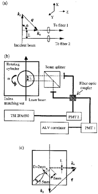
FIG. 1.: (a) Scattering geometry for the velocity difference measurement. $\bf k_{i}$, incident wave vector; $\bf k_{s}$, scattered wave vector; and ${\bf q}={\bf k_{s}}-{\bf k_{i}}$. (b) Experimental setup for the velocity difference measurement in rigid body rotation. (c) Flow cell and optical arrangement for a jet flow.

As shown in Fig. 1(b), an incident beam from a Nd:YVO₄ laser with a power range of 0.5-2W and a wavelength of $\lambda$=532 nm is directed to a flow cell by a lens. With the aid of a large beam splitting cube, two single-mode, polarization-maintaining (PM) fibers collect the scattered light from two different spots along the laser beam with a separation $L$. The two PM fibers are connected to a fiber-optic coupler (purchased from OZ Optics[11]), which combines the light from the two input fibers and split the resultant light evenly into two output fibers. A graded index lens is placed at each end of the fiber to collimate the light entering (or exiting from) the fiber core. Each input fiber is mounted on a micrometer-controlled translation stage and the distance $L$ can be adjusted in a range of 0-25 mm in steps of 0.01 mm. The output fibers of the optical coupler are connected to two photomultiplier tubes (PMT1 and PMT2). PMT1 is operated in the digital mode and its output signal is fed to a digital correlator (ALV-5000). PMT2 is operated in the analogue mode and its output signal is fed to a LDV signal processor (TSI IFA655). An oscilloscope connected to PMT2 directly views the analogue signals. A low-noise preamplifier (Stanford Research SR560) further amplifies the analogue output of PMT2 before it goes to the LDV signal processor.

As shown in Fig. 1(a), the electric fields detected by each input fiber sum in the coupler and consequently interfere. In the experiment, we obtain the beat frequency, $\Delta\omega_{2}={\bf q}\cdot{\bf v}_{1}-{\bf q}\cdot{\bf v}_{2}={\bf q}\cdot\delta{\bf v}(L)$, in two different ways. One way is to measure the intensity auto-correlation function $g(\tau)$ in Eq. (1). With the ALV correlator, it takes $\sim 1$ minute to collect the data with an adequate signal-to-noise ratio. The other way is to use the LDV signal processor to measure the instantaneous beat frequency $\Delta\omega_{2}$, giving velocity differences in real time. The LDV signal processor is essentially a very fast correlator and thus requires the beat signal to be large enough so that no signal averaging is needed. In the experiment to be discussed below, we use both methods to analyze the beat signals and compare the results.

It has been shown that the correlation function $g(\tau)$ has the form:[5]

$$g(\tau) = 1+\frac{I_{1}^{2}+I_{2}^{2}}{(I_{1}+I_{2})^{2}}G_{s}(\tau)+\frac{2I_{1}I_{2}}{(I_{1}+I_{2})^{2}}G_{c}(\tau)$$ (3)

$$= 1+b_{s}G_{s}(\tau)+b_{c}G_{c}(\tau),$$ (4)

where $I_{1}$ and $I_{2}$ are the light intensities from the two input fibers. When $I_{1}=I_{2}$, one finds $b_{s}=b_{c}=0.5$. If one of the input fibers is blocked (i.e., $I_{2}=0$), we have $g(\tau)=1+G_{s}(\tau)$, where $G_{s}(\tau)$ is the self-beat correlation function for a single fiber. When the separation L between the two input fibers is much larger than the spot size viewed by each fiber, the cross-beat correlation function $G_{c}(\tau)$ takes the form

$$G_{c}(\tau)\simeq G_{s}(\tau)\int_{-\infty}^{+\infty}d\delta v~{}P(\delta v)\cos(q\delta v(L)\tau).$$ (5)

Two flow cells are used in the experiment. The first one is a cylindrical cuvette having an inner diameter of 2.45 cm and a height of 5 cm. The cuvette is top mounted on a geared motor, which produces smooth rotation with an angular velocity $\omega=2.5~{}rad/s$. The cell is filled with 1,2-propylene glycol, whose viscosity is 40 times larger than that of water. The whole cell is immersed in a large square index-matching vat, which is also filled with 1,2-propylene glycol. The flow field inside the cell is a simple rigid body rotation. With the scattering geometry shown in Fig. 1(b), the beat frequency is given by $\Delta\omega_{2}=k_{s}\omega L$ with $k_{s}=2\pi n/\lambda$. The sample cell is seeded with a small amount of polystyrene latex spheres. For the correlation measurements, we use small seed particles of $1.0~{}\mu m$ in diameter. By using the small seed particles, one can have more particles in the scattering volume even at low seeding densities. This will reduce the amplitude of the number fluctuations caused by a change in the number of particles in each scattering volume. The particle number fluctuations can produce incoherent amplitude fluctuations to the scattered light and thus introduce an extra (additive) decay to $g(\tau)$.[16] Large particles $4.75~{}\mu m$ in diameter are used to produce higher scattering intensity for instantaneous Doppler burst detection. Because the densities of the latex particles and the fluid are closely matched, the particles follow the local flow well and they do not settle much.

The second flow cell shown in Fig. 1(c) is used to generate a jet flow in a $9cm\times 9cm$ square vat filled with quiescent water. The circular nozzle has an outlet 2 mm in diameter and the tube diameter before the contraction is 5.5 mm. The nozzle is immersed in the square vat and a small pump is used to generate a jet flow at a constant flow rate $0.39~{}cm^{3}/s$. The mean velocity at the nozzle exit is $12.4~{}cm/s$ and the corresponding Reynolds number is Re=248. This value of Re is approximately three times larger than the turbulent transition Reynolds number, $Re_{c}\simeq 80$, for a round jet.[12] Because of the large area contraction (7.6:1), the bulk part of the velocity profile at the nozzle exit is flat. This uniform velocity profile vanishes quickly, and a Gaussian-like velocity profile is developed in the downstream region, 2-20 diameters away from the nozzle exit.[13] As shown in Fig. 1(c), the direction of the momentum transfer vector $\bf q$ (and hence the measured velocity difference) is parallel to the jet flow direction, but the separation L is at an angle of $45^{o}$ to that direction.

B Measurement of the local velocity

In the measurement of the velocity difference, we use two input fibers to collect the scattered light with the same $\bf q$ (i.e. at the same scattering angle) but from two spatially separated regions in the flow. We now show that with a different optical arrangement, the fiber-optic method can also be used to measure the instantaneous local velocity ${\bf v}({\bf x},t)$. Instead of collecting light from two spatially separated regions with the same $\bf q$, we use the two input fibers to collect light from a common scattering volume in the flow but with two different momentum transfer vectors $\bf q_{1}$ and $\bf q_{2}$ (i.e. at two different scattering angles). Figure 2(a) shows the schematic diagram of the scattering geometry. The collected signals at the two scattering angles are combined by a fiber-optic coupler, and the resultant light is modulated at the Doppler beat frequency:[14] $\Delta\omega_{1}={\bf q_{1}}\cdot{\bf v}-{\bf q_{2}}\cdot{\bf v}=\Delta{\bf q}\cdot{\bf v}({\bf x})$, where $\Delta{\bf q}=\bf q_{1}-\bf q_{2}$. The magnitude of $\Delta{\bf q}$ is given by $\Delta q=(4\pi n/\lambda)\sin(\alpha/2)$, with $\alpha$ being the acceptance angle between the two fibers.

The principle of using the scattered light at two different scattering angles to measure the local velocity has been demonstrated many years ago.[14] What is new here is the use of the fiber-optic coupler for optical mixing. The fiber-optic technique simplifies the standard LDV optics considerably. As shown in Fig. 2(b), in the standard LDV arrangement the two incident laser beams form interference fringes at the focal point. When a seed particle traverses the focal region, the light scattered by the particle is modulated by the interference fringes with a frequency,[15] $\Delta\omega_{1}={\bf q_{1}}\cdot{\bf v}-{\bf q_{2}}\cdot{\bf v}=\Delta{\bf q}\cdot{\bf v}({\bf x})$. The magnitude of $\Delta{\bf q}$ has the same expression $\Delta q=(4\pi n/\lambda)\sin(\alpha/2)$ as shown in the above, but $\alpha$ now becomes the angle between the two incident laser beams. The main difference between the standard LDV and the new fiber-optic method is that the former employs two incident laser beams and a receiving fiber [Fig. 2(b)], while the latter uses only one incident laser beam and two optical fibers to measure each velocity component [Fig. 2(a)]. Consequently, the beat frequency $\Delta\omega_{1}$ in Fig. 2(a) is independent of the direction ($\bf k_{i}$) of the incident laser beam, whereas in Fig. 2(b) it is independent of the direction ($\bf k_{s}$) of the receiving fiber.

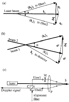
FIG. 2.: (a) One-beam scattering geometry for the local velocity measurement. $\bf k_{i}$, incident wave vector; $({\bf k_{s}})_{1}$ and $({\bf k_{s}})_{2}$, two scattered wave vectors; ${\bf q}_{1}=({\bf k_{s}})_{1}-{\bf k_{i}}$; ${\bf q}_{2}=({\bf k_{s}})_{2}-{\bf k_{i}}$; $\Delta{\bf q}={\bf q}_{2}-{\bf q}_{1}$. (b) Two-beam scattering geometry for the local velocity measurement. $({\bf k_{i}})_{1}$ and $({\bf k_{i}})_{2}$, two incident wave vectors; $\bf k_{s}$, scattered wave vector; ${\bf q}_{1}={\bf k_{s}}-({\bf k_{i}})_{1}$; ${\bf q}_{2}={\bf k_{s}}-({\bf k_{i}})_{2}$; $\Delta{\bf q}={\bf q}_{2}-{\bf q}_{1}$. (c) Schematic diagram of a one-beam probe for the local velocity measurement. S, measuring point; P, lens; M, frequency modulator; C, fiber-optic coupler.

With the one-beam scheme, one can design various optical probes for the local velocity measurement. Figure 2(c) shows an example, which would replace the commercial LDV probe by reversing the roles of the transmitter and receiver. The two input fibers aim at the same measuring point S through a lens P, which also collects the back-scattered light from S. The frequency modulator M shifts the frequency of the light collected by the input fiber 1, before it is combined via the fiber-optic coupler C with the light collected by the input fiber 2. The resultant light from an output fiber of the coupler contains the beat frequency $\Delta\omega_{1}$ and is fed to a photodetector. Because the measured $\Delta\omega_{1}$ is always a positive number, one cannot tell the sign of the local velocity when zero velocity corresponds to a zero beat frequency. The frequency shift by the modulator M causes the interference fringes to move in one direction (normal to the fringes) and thus introduces an extra shift frequency to the measured beat frequency. This allows us to measure very small velocities and to determine the sign of the measured local velocity relative to the direction of the fringe motion (which is known).[15] The other output fiber of the coupler can be used as an alignment fiber, when it is connected to a small He-Ne laser. With the reversed He-Ne light coming out of the input fibers, one can directly observe the scattering volume viewed by each input fiber and align the fibers in such a way that only the scattered light from the same measuring point S is collected.

The one-beam probe has several advantages over the usual two-beam probes. To measure two orthogonal velocity components in the plane perpendicular to the incident laser beam, one only needs to add an extra pair of optical fibers and a coupler and arrange them in the plane perpendicular to that shown in Fig. 2(c) (i.e., rotate the two-fiber plane shown in Fig. 2(c) by $90^{o}$). With this arrangement, the four input fibers collect the scattered light from the same scattering volume but in two orthogonal scattering planes. Because only one laser beam is needed for optical mixing, a small single-frequency diode laser, rather than a large argon ion laser, is sufficient for the coherent light source. In addition, the one-beam arrangement does not need any optics for color and beam separations and thus can reduce the manufacturing cost considerably. With the one-beam scheme, one can make small invasive or non-invasive probes consisting of only three thin fibers. One can also make a self-sustained probe containing all necessary optical fibers, couplers, photodetectors, and a signle-frequency diode laser.

III Results and Discussion

A Velocity difference measurements

We first discuss the measurements of the velocity difference in rigid body rotation. Figure 3(a) shows a sample oscilloscope trace of the analogue output from PMT2 when the separation L=1.0 mm. The signal is amplified 1250 times and band-pass-filtered with a frequency range of 1-10 kHz. This oscilloscope trace strongly resembles the burst signals in the standard LDV. The only difference is that the signal shown in Fig. 3(a) results from the beating of two moving particles separated by a distance L. Figure 3(a) thus demonstrates that the beat signal between the two moving particles is large enough that a standard LDV signal processor can be used to measure the instantaneous velocity difference $\delta v(\ell,t)$ in real time.

Figure 3(b) shows the measured beat frequency $\Delta\omega_{2}$ as a function of separation L. The circles are obtained from the oscilloscope trace and the triangles are obtained from the intensity correlation function $g(\tau)$. The two measurements agree well with each other. The solid line is the linear fit $\Delta\omega_{2}=41.78L~{}(10^{3}~{}rad/s)$, which is in good agreement with the theoretical calculation $\Delta\omega_{2}=k_{s}\omega L=42.28L~{}(10^{3}~{}rad/s)$. This result also agrees with the previous measurements by Du et al.[5] Because $\Delta\omega_{2}$ increases with L, one needs to increase the laser intensity at large values of L in order to resolve $\Delta\omega_{2}$. The average photon count rate should be at least twice the measured beat frequency.

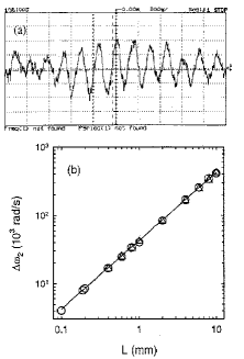
FIG. 3.: (a) Oscilloscope trace of a typical beat burst between two moving particles separated by a distance L=1.0 mm. The signal is obtained in rigid body rotation. (b) Measured beat frequency $\Delta\omega_{2}$ as a function of separation L. The circles are obtained from the oscilloscope trace and the triangles are obtained from the intensity correlation function $g(\tau)$. The solid line shows a linear fit to the data points.

We now discuss the time series measurements of $\delta v(L,t)$ in a jet flow using the LDV signal processor. The jet flow has significant velocity fluctuations as compared with the laminar rigid body rotation. The measuring point is in the developing region of the jet flow, 3 diameters away from the nozzle exit and is slightly off the centerline of the jet flow. Figure 4 shows the measured histogram $P(\delta v)$ of the velocity difference $\delta v(L,t)$ in the jet flow, when the separation L is fixed at L=0.5 mm (circles) and L=0.8 mm (squares), respectively. It is seen that the measured $P(\delta v)$ has a dominant peak and its position changes with L. Because $\delta v(L,t)$ increases with L, the peak position moves to the right for the larger value of L. The solid curve in Fig. 4 is a Gaussian fit to the data points with L=0.5 mm. The obtained mean value of $\delta v(L,t)$ is $\langle\delta v\rangle=1.87~{}cm/s$ and the standard deviation $\sigma=0.171~{}cm/s$. At L=0.8 mm, the measured $P(\delta v)$ peaks at the value $\langle\delta v\rangle=2.73~{}cm/s$.

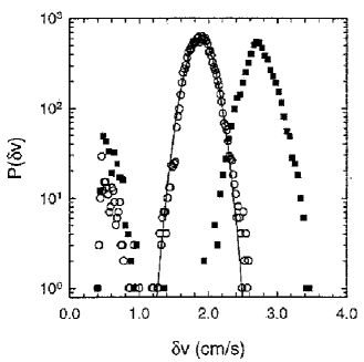
FIG. 4.: Measured histogram $P(\delta v)$ of the velocity difference $\delta v(L,t)$ in the jet flow. The values of L are: L=0.5 mm (circles) and 0.8 mm (squares). The solid curve is a Gaussian fit to the circles.

In the above discussion, we have assumed that each input fiber sees only one particle at a given time and the beat signal comes from two moving particles separated by a distance L. In fact, when the seeding density is high, each input fiber may see more than one particle at a given time. The scattered light from these particles can also beat and generate a self-beat frequency proportional to $\delta v(\ell_{0})$, where $\ell_{0}\simeq 0.15~{}mm$ is the laser spot size viewed by each input fiber.[5] The self-beating gives rise to a small peak on the left side of the measured $P(\delta v)$. Note that the peak position is independent of L, because $\delta v(\ell_{0})$ is determined only by $\ell_{0}$, which is the same for both measurements. It is seen from Fig. 4 that the cross-beating is dominant over the self-beating under the current experimental condition.

The intensity correlation function $g(\tau)$ is also used to analyze the beat signal. In the experiment, we measure the histogram $P(\delta v)$ and $g(\tau)$ simultaneously, so that Eq. (5) can be examined in details. Figure 5 shows the measured $g(\tau)-1$ (circles) as a function of delay time $\tau$ at L=0.5 mm. The squares are the self-beat correlation function $G_{s}(\tau)$ obtained when one of the input fibers is blocked. As shown in Fig. 4, the measured $P(\delta v)$ has a Gaussian form and thus the integration in Eq. (5) can be carried out. The final form of $g(\tau)$ becomes

$$g(\tau)=1+G_{s}(\tau)\left[b_{s}+b_{c}\cos[q\langle\delta v\rangle\tau]e^{-(q\sigma\tau)^{2}/2}\right].$$ (6)

The solid curve in Fig. 5 is a plot of Eq. (6) with $b_{s}=0.5$ and $b_{c}=0.13$. The values of $\langle\delta v\rangle$ and $\sigma$ used in the plot are obtained from the Gaussian fit shown in Fig. 4. It is seen that the calculation is in good agreement with the measured $g(\tau)$.

The fitted value $b_{s}=0.5$ agrees with the expected value at $I_{1}=I_{2}$. The value of $b_{c}$ would be 0.5 if the collected signals from the two input fibers were fully coherent and the fiber-optic coupler mixed them perfectly. The fact that the fitted value of $b_{c}$ is smaller than 0.5 indicates that the collected signals are not fully correlated. This is caused partially by the fact that in the present experiment the scattered light suffers relatively large number fluctuations resulting from a changing number of particles in the scattering volume. These number fluctuations produce incoherent amplitude fluctuations to the scattered light and thus introduce an extra (additive) decay to $g(\tau)$.[16] Because the beam crossing time (proportional to the beam diameter) is much longer than the Doppler beat time $1/\Delta\omega_{2}$ (proportional to the wavelength of the scattered light), the slow decay due to the number fluctuations can be readily identified in the measured $g(\tau)$. This decay has an amplitude 0.4 and has been subtracted out from the measured $g(\tau)$ shown in Fig. 5.

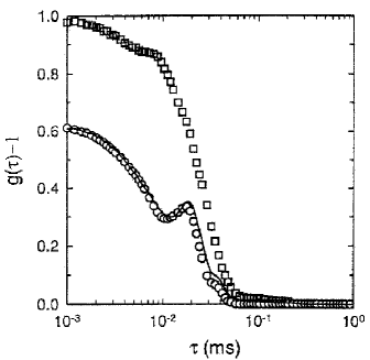
FIG. 5.: Measured intensity correlation function $g(\tau)-1$ as a function of delay time $\tau$ at L=0.5 mm (open circles). The squares are obtained when one of the input fibers is blocked. The solid curve is a plot of Eq. (5).

It is shown in Eq. (6) that to accurately measure the mean velocity difference $\langle\delta v\rangle$, the beat frequency $\Delta\omega_{2}=q\langle\delta v\rangle$ must be larger than the decay rate $\Gamma_{s}\simeq q\delta v(\ell_{0})$ for $G_{s}(\tau)$ and also larger than the decay rate $\Gamma_{c}\simeq q\sigma$ resulting from the fluctuations of the velocity difference. From the measurements shown in Figs. 4 and 5, we find $\Gamma_{s}\simeq 1.33\times 10^{5}~{}s^{-1}$ and $\Gamma_{c}\simeq 3.8\times 10^{4}~{}s^{-1}$, which are indeed smaller than the beat frequency $\Delta\omega_{2}\simeq 4.15\times 10^{5}~{}s^{-1}$. Because $g(\tau)$ contains a product of $G_{s}(\tau)$ and $\exp[-(q\sigma\tau)^{2}/2]$ [see Eq. (6)], its decay is determined by the faster decaying function. It is seen from Fig. 5 that the decay of $g(\tau)$ is controlled by $G_{s}(\tau)$, which decays faster than $\exp[-(q\sigma\tau)^{2}/2]$. It should be noted that in the measurements shown in Fig. 4, the beat signals are analogue ones and we have used a band-pass filter together with a LDV signal analyzer to resolve the beat frequency. Consequently, many low-frequency self-beat signals are filtered out. This low-frequency cut-off is apparent in Fig. 4. The measurements of $g(\tau)$, on the other hand, are carried out in the photon counting mode, and therefore the measured $g(\tau)$ is sensitive to all the self-beat signals as well as the cross beat signals. With a simple counting of particle pairs, we find that the probability for cross beating is only twice larger than that for the self-beating.

B Local velocity measurements

We now discuss the local velocity measurements using the new optical arrangement shown in Fig. 2(a). The velocity measurements are conducted on a freely suspended flowing soap film driven by gravity. Details about the apparatus has been described elsewhere,[17, 18, 19] and here we mention only some key points. $2\%$ solution of detergent and water is introduced at a constant rate between two long vertical nylon wires, which are held apart by small hooks. The width of the channel (i.e., the distance between the two nylon wires) is 6.2 cm over a distance of 120 cm. The measuring point is midway between the vertical wires. The soap solution is fed, through a valve, onto an apex at the top of the channel. The film speed $\bar{v}$, ranging from 0.5 to 3 m/s, can be adjusted using the valve. The soap film is approximately 2-6 $\mu m$ in thickness and is seeded with micron-sized latex particles, which scatter light from a collimated laser beam. The light source is an argon-ion laser having a total power of 1W. The incident laser beam is oriented perpendicular to the soap film and the scattered light is collected in the forward direction.

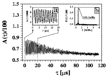
FIG. 6.: Measured intensity autocorrelation function $A(\tau)$ as a function of delay time $\tau$ with the measuring time T=30 ms. The inset (a) shows an enlarged portion of $A(\tau)$ for small values of $\tau$ up to $\tau=20~{}\mu s$. The inset (b) shows the frequency power spectrum $P(f)$ of the measured $A(\tau)$.

To measure the rapidly changing beat frequency $\Delta\omega_{1}$, we build a fast digital correlator board for PC.[20] With a fast sampling rate $f_{s}$, the plug-in correlator board records the time-varying intensity I(t) (number of TTL pulses from the photomultiplier tube per sample time) over a short period of time T and then calculates the (unnormalized) intensity autocorrelation function, $A(\tau)=\langle I(t+\tau)I(t)\rangle$. Figure 6 shows an example of the measured $A(\tau)$ as a function of delay time $\tau$ with T = 30 ms and $f_{s}=14.32$ MHz. Because the burst signal I(t) is a periodic function of t, the measured $A(\tau)$ becomes an oscillatory function of $\tau$. The frequency of the oscillation apparent in the inset (a) is the beat frequency $\Delta\omega_{1}$. The amplitude of the oscillation decays at large $\tau$. The inset (b) shows the power spectrum $P(f)$ of the measured $A(\tau)$; it reveals a dominant peak at 755.1 kHz. The power spectrum is obtained using a fast Fourier transform (FFT) program.[21]

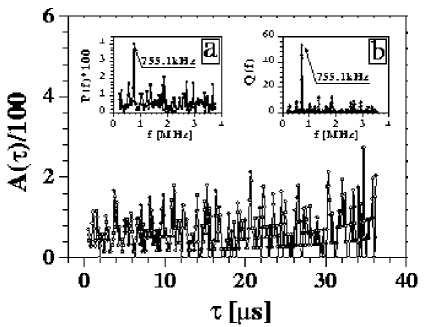
FIG. 7.: Measured intensity autocorrelation function $A(\tau)$ as a function of delay time $\tau$ with the measuring time T=50 $\mu s$. The inset (a) shows the frequency power spectrum $P(f)$ obtained by FFT. The inset (b) shows the frequency spectrum $Q(f)$ obtained by the Scargle-Lomb method.

To increase the sampling rate of the velocity measurements, one needs to keep the measuring time T for each $A(\tau)$ as short as possible. The signal-to-noise ratio for $A(\tau)$ decreases with shorter measuring time T and with lower mean photon count rate, which was $\sim 1$ MHz in the present experiment. It is found that the shortest useful measuring time $T_{c}$ is roughly $50~{}\mu s$. For this value of T, $A(\tau)$ is quite noisy and the corresponding peak in $P(f)$ becomes less pronounced [see Fig. 7 and inset (a)]. It is worth mentioning that if one only wants to know the periodicity of a function, rather than its actual power at different frequencies, the Scargle-Lomb method[22] is a better alternative to FFT. This method, which does not require evenly spaced sampling, compares the measured data with known periodic signals using the least-square fitting procedure and determines the relevant frequencies by the goodness of the fit $Q(f)$. It can even utilize the uneven sampling to further increase the Nyquist frequency. As shown in Fig. 7(b), the Scargle-Lomb method can still clearly identify the periodicity of the signal, even when the power spectrum $P(f)$ [Fig. 7(a)] becomes less reliable. The total time required for the measurement of the characteristic frequency is less than 1 ms. Using the correlator board together with an average speed PC (300 MHz), we are able to conduct accurate measurements of the local velocity with a sampling rate up to 1 kHz.

IV Summary

We have developed new optical arrangements with two single-mode input fibers and a fiber-optic coupler to measure the local velocity ${\bf v}({\bf x})$ and the velocity difference, $\delta{\bf v}({\bf\ell})={\bf v}({\bf x}+{\bf\ell})-{\bf v}({\bf x})$, between two spatial points separated by a distance $\ell$. The fibers and the coupler are polarization preserving to guarantee a high signal-to-noise ratio. To measure the velocity difference $\delta{\bf v}({\bf\ell})$, the two input fibers are used to collect the scattered light with the same momentum transfer vector $\bf q$ but from two spatially separated regions in a flow. These regions are illuminated by a single coherent laser beam, so that the collected signals interfere when combined via the fiber-optic coupler. The resultant light received by a photomultiplier tube therefore contains the beat frequency $\Delta\omega_{2}={\bf q}\cdot\delta{\bf v}(\ell)$. We analyzed the beat signals using two different devices and compared the results. First, the intensity auto-correlation function $g(\tau)$ was measured using a digital correlator. Secondly, a standard LDV signal processor was used to determine the instantaneous beat frequency $\Delta\omega_{2}$. With this device, $\delta{\bf v}({\bf\ell,t})$ can be obtained in real time. The technique can be further developed to measure one component of the local flow vorticity vector ${\vec{\omega}}({\bf x},t)={\bf\nabla}\times{\bf v}({\bf x},t)$.[23]

To measure the instantaneous local velocity itself, one needs only to reorient the two fibers so that they point to the same scattering volume. With this optical arrangement, we have three alternatives to measure a velocity component. They employ (i) an analog photodetector and a standard LDV signal processor (burst detector), (ii) a commercial photon correlator, such as that made by ALV, and finally (iii) a home-made digital correlator. This latter device completes a velocity measurement in less than 1 ms and is orders of magnitude cheaper than the other two alternatives. The new fiber-optic method has several advantages over the standard LDV and can be used widely in the general area of fluid dynamics. Because only one laser beam is needed to obtain two velocity components, a compact single-frequency diode laser can replace a large multi-frequency argon-ion laser. By eliminating the color and beam separation units in the standard LDV, the one-beam scheme is less costly to implement. With more optical fiber pairs and couplers, one can carry out multi-point and multi-component velocity measurements in various turbulent flows.

REFERENCES

- [1] U. Frisch, Turbulence: the legacy of A. N. Kolmogorov (Cambridge University Press, Cambridge, UK, 1995).
- [2] K. R. Sreenivasan, “Fluid turbulence,” Rev. Mod. Phys, 71, S383-395 (1999).
- [3] G. I. Taylor, “The spectrum of turbulence,”Pro. R. Soc. London A, 164, 476-490 (1938).
- [4] T. Narayanan, C. Cheung, P. Tong, W. I. Goldburg, and X.-L. Wu, “Measurement of the velocity difference by photon correlation spectroscopy: an improved scheme,”Applied Optics, 36, 7639-7644 (1997).
- [5] Yixue Du, B. J. Ackerson, and P. Tong, “Velocity difference measurement with a fiber-optic coupler,” J. Opt. Soc. Am. A. 15, 2433-2439 (1998).
- [6] B. J. Berne and R. Pecora, Dynamic light scattering (Wiley, New York, 1976).
- [7] P. Tong, W. I. Goldburg, C. K. Chan, and A. Sirivat, “Turbulent transition by photon correlation spectroscopy,” Phys. Rev. A, 37, 2125-2133 (1988).
- [8] H. K. Pak, W. I. Goldburg, and A. Sirivat, “Measuring the probability distribution of the relative velocities in grid-generated turbulence,”Phys. Rev. Lett. 68, 938-941 (1992).
- [9] P. Tong and Y. Shen, “Relative velocity fluctuations in turbulent Rayleigh-Bénard convection,” Phys. Rev. Lett. 69, 2066-2069 (1992).
- [10] H. Kellay, X.-l. Wu, and W. I. Goldburg, “Experiments with turbulent soap films,”Phys. Rev. Lett. 74, 3975-3978 (1995).
- [11] Oz Optics Ltd, 219 Westbrook Road, Carp ON Canada, K0A 1L0 (http://ozoptics.com).
- [12] J. W. Daily and D. R. F. Harleman, Fluid Dynamics, p.421 (Addison-Wesley, Reading, MA, 1966).
- [13] F. M. White, Viscous Fluid Flow, p.470 (McGrn-Hill, New York, 1991).
- [14] F. Durst and J. H. Whitelaw, “Optimization of optical anemometers,” Proc. of Royal Soc. A. 324, 157-181 (1971).
- [15] L. E. Drain, The laser Doppler technique (John Wiley Sons, New York, 1980).
- [16] P. Tong, K. -Q. Xia, and B. J. Ackerson, “Incoherent cross-correlation spectroscopy,”J. Chem. Phys. 98, 9256-9264 (1993).
- [17] M. A. Rutgers, X. L. Wu, R. Bagavatula, A. A. Peterson, and W. I. Gouldburg, “Two-dimensional velocity profiles and laminar boundary layers in flowing soap films,”Phys. Fluids 8, 2847 (1997).
- [18] W. I. Goldburg, A. Belmonte, X. L. Wu, and I. Zusman, “Flowing soap films: a laboratory for studying two-dimensional hydrodynamics,”Physica A 254, 231-247 (1998).
- [19] V. K. Horváth, R. Crassman, W. I. Goldburg, and X. L. Wu, “Hysteresis at low Reynolds number: Onset of two-dimensional vortex shedding”, Phys. Rev. E 61, R4702-4705 (2000) cond-mat/9903067.
- [20] For a full description of the correlator board, seehttp://karman.phyast.pitt.edu/horvath/corr/. The total cost for the correlator board is less than . The device can be duplicated for non-profit applications without permission.
- [21] see, e.g., W. H. Press, B. P. Flannery, S. A. Teukolsky, and W. T. Vetterling, Numerical Recipes, 2nd edition (Cambridge University Press, UK, 1992).
- [22] J. D. Scargle, “Studies in astronomical time series analysis III.”Astrophy. J. 343, 874-887 (1989).
- [23] S. H. Yao, P. Tong, and B. J. Ackerson, “Instantaneous vorticity measurements using fiber-optic couplers,” manuscript available from the authors.