^(a) The University of New South Wales, Sydney, Australia
^(b) Institute of Physics, The University of St Petersburg, Russia

ATOMIC ANTENNA MECHANISM IN HHG AND ATI

1 Introduction

This paper reviews recent development of the atomic antenna, a theoretical framework which describes a number of laser-induced multiphoton phenomena in atoms. The localization of atomic electrons inside an atom drastically suppresses their interaction with a laser field. For many processes this circumstance favors multistep mechanisms when at first one of atomic electrons is released from an atom by the field. After that an interaction of the ejected electron with the laser field results in absorption of energy from the field and its accumulation in the form of the electron wiggling energy and ATI energy. It is very essential that the energy absorbed by the electron can be transferred to the parent atomic core via an inelastic collision of the primarily ejected electron with the atom. The collision may trigger a number of phenomena including high harmonic generation (HHG), enhancement of above-threshold ionization (ATI), production of multiply charged ions. In this physical picture the absorption of energy from the field takes place in the region of large separations from an atom, where the electron-laser interaction dominates over the electron-core potential. This circumstance results in dramatic enhancement of the probability of multiphoton processes. Such a scenario of photoabsorption was suggested, apparently for the first time, in Ref. [1]. Later the idea was rediscovered by several authors in different contexts [2, 3, 4]. In current literature the above described sequence of events is often referred to as the rescattering, the three-step mechanism, or even the simpleman model. The term atomic antenna, suggested in Ref. [1], refers to the fact that the firstly emitted electron plays a role similar to an aerial in conventional radio devices, enhancing the absorption.

It is very important that the physical picture drawn above can be implemented not only as a model, but also as a clear and rigorous quantum formalism. In this paper we outline two convenient ways to implement the atomic antenna idea. The one originating from Ref. [1] is called the factorization technique. It was formulated in detail in Ref. [5] and recently applied to HG in Refs. [6, 7]. We discuss also another, complimentary technique, which is referred to below as the method of effective ATI channels. It is close in spirit to the approach developed previously by Lewenstein et al [8, 9] and can in turn be linked to the Corcum model [2]. From the first glance, these two schemes differ very significantly. However, we prove their identity by demonstrating that they describe the same physical idea from different points of view.

The paper is organized as follows. Section 2 describes the factorization technique which allows one to present the amplitude of the ”complicated” multiphoton process as a product of the amplitudes of much more simple, ”elementary” processes. Section 3 is devoted to the concept of effective ATI channels, which provides important insights into the physical nature of complicated multiphoton processes. We derive the effective ATI channels from the factorization technique revealing close links between the two approaches. Section 4 describes two important examples of ”elementary” processes: one of them is the photoionization, another one is the electron-atom collision in a laser field which results in the generation of the high-energy quanta. These two ”elementary” processes are vital for description of HG in the framework of the factorization technique. Sections 5, 6 are devoted to several examples illustrating numerically an accuracy of methods developed for HHG and ATI. A number of results reported in this paper are derived neglecting the Coulomb field of the residual atomic particle which influence the active atomic electron. This approach is well justified for negative ions, but needs to be modified for the processes with neutral atoms. Section 7 exposes our recent progress based on the eikonal approach which allows us to take into account the Coulomb field. The concluding Section 8 summarizes the results. The atomic units are used throughout the paper unless indicated otherwise.

2 Factorization technique

The factorization technique of Ref. [5] can be applied to a number of multiphoton processes. In this section our attention is restricted to an important example of HG which has been recently considered by the present authors [6, 7]. We concentrate on the linearly polarized laser field

$${\bf F}(t)={\bf F}\cos\omega t$$ (1)

that creates the external potential $V(t)={\bf F}(t)\cdot{\bf r}$ acting on atomic electrons. Using the second order time-dependent perturbation theory one can present the amplitude of HHG $d_{N}^{+}$ in the single-active-electron approximation in the following form

$$d_{N}^{+}=-\,\frac{i}{T}\int_{0}^{T}dt\,\int_{-\infty}^{t}dt^{\prime}\,\langle\phi_{a}(t)\,|\,\exp(i\Omega t)\,U\,G(t,t^{\prime})\,V(t^{\prime})\,|\,\phi_{a}(t^{\prime})\rangle~{}.$$ (2)

Here the brackets $\langle\,|\,|\,\rangle$ imply integration over coordinates, $T=2\pi/\omega$ is the laser period. The initial-state wave function is

$$\phi_{a}({\bf r},t)=\phi_{a}({\bf r})\exp(-iE_{a}t)$$ (3)

where $E_{a}=-\kappa^{2}/2$ is the bound state energy and $\phi_{a}({\bf r})$ is the corresponding atomic eigenfunction. The potential $U=\mbox{\boldmath$\epsilon$}\cdot{\bf r}$ accounts for production of the high harmonic with the frequency $\Omega=N\omega$ and the polarization $\epsilon$. The Green function $G(t,t^{\prime})$ describes the electron propagation in the intermediate state. The amplitude (2) takes into account only a sequence of events in which HHG follows the absorption of the necessary energy from the laser field. A number of omitted, the so called time-reversed sequences, is strongly suppressed due to multiphoton nature of the process.

Neglecting the potential of the atomic core (a possible way to lift this approximation is considered in Section 7), one can present the Green function via a complete set of the Volkov wave functions $\phi_{\bf p}({\bf r},t)$ that account for the electron dressing by the laser field

$$G({\bf r},t;{\bf r}^{\prime},t^{\prime})=\int\,\phi_{\bf p}({\bf r},t)\phi_{\bf p}^{*}({\bf r}^{\prime},t^{\prime})\,\frac{d^{3}p}{(2\pi)^{3}}~{},$$ (4)

$$\phi_{\bf p}({\bf r},t)=\exp\left\{i\left[\left({\bf p}+\frac{\bf F}{\omega}\sin\omega t\right)\cdot{\bf r}-\,\frac{1}{2}\int^{t}\left({\bf p}+\frac{\bf F}{\omega}\sin\omega\tau\right)^{2}d\tau\right]\right\}~{}.$$ (5)

The multiphoton nature of the problem makes the phases of the integrand in (2) to vary rapidly with $t$, $t^{\prime}$. This circumstance allows one to use the saddle-point approximation for integrations over the time variables. After the accurate integration over the momenta ${\bf p}$ in (4), see details in [5, 6, 7], it is possible to show that (2), (4), (5) lead to the following convenient presentation of the HHG amplitude

$$d^{+}_{N} = 2\,\sum_{m}\,d^{+}_{Nm}~{},$$ (6)

$$d^{+}_{Nm} = A_{m\,\mu_{0}}({\bf K}_{m})\,B_{N\,m\mu_{0}}({\bf K}_{m})~{}.$$ (7)

Each term in (6) is written as a product of two amplitudes of physical, fully accomplished and observable processes; no ”off-shell” entities appear. Therefore Eqs. (6), (7) clearly demonstrate the stepwise character of the process. The first step is described by the first factor $A_{m\,\mu_{0}}({\bf K}_{m})$ which is an amplitude of physical ATI process when after absorption of $m$ laser photons the active electron acquires a translational momentum ${\bf p}={\bf K}_{m}$. In the Keldysh-type approximation this amplitude can be evaluated using the saddle-point technique discussed in Section 4. The subscript $\mu_{0}$ in $A_{m\,\mu_{0}}$ specifies the contribution of one particular saddle point in $t^{\prime}$ integration, see more details in Section 4. The other factor, $B_{N\,m\mu_{0}}({\bf K}_{m})$, is a combined amplitude of the second and third steps, which are the propagation and laser assisted recombination (PLAR). It can be further factorised into the propagation factor $1/R_{m\mu_{0}}$ describing the second step and the amplitude of the third step, which is the laser assisted recombination (LAR), $C_{Nm}({\bf K}_{m})$:

$$B_{N\,m\mu_{0}}({\bf K}_{m})\simeq\frac{1}{R_{m\mu_{0}}}\,C_{Nm}({\bf K}_{m})~{}.$$ (8)

$R_{m\mu_{0}}$ is merely an approximate expression for the distance passed by the active electron in course of its laser-induced wiggling motion

$$\frac{1}{R_{m\,\mu_{0}}}=-\,\frac{\omega^{2}}{F\cos\omega t^{\prime}_{m\mu_{0}}}~{}.$$ (9)

The amplitude $C_{Nm}({\bf p})$ of the physical LAR process describes the laser assisted recombination, i.e. transition of an electron with momentum ${\bf p}$ from the continuum to the bound state. Since the continuum state is laser-dressed, the recombining electron can emit the $N$-th harmonic photon, gaining necessary extra energy from the laser field. More details on LAR amplitude are given in Section 4.

The summation in formula (6) runs over a number of photons $m$ absorbed on the first step of the process when the active electron is released. In other words one can say that the energy conservation constraint selects the discrete set of ATI channels in the laser-dressed continuum. These channels serve as intermediate states for the three-step HG process. In a given channel the electron has translational momentum ${\bf K}_{m}$ with the absolute value defined by

$$K_{m}=\sqrt{2\left(m\omega-U_{p}+E_{a}\right)}~{}.$$ (10)

Here $U_{p}\equiv F^{2}/(4\omega^{2})$ is the well-known ponderomotive potential. ATI plays a role of the first stage of HHG process only if the electron momentum has specific direction, namely ${\bf K}_{m}$ is directed along ${\bf F}$. This ensures eventual electron return to the core that makes the final step, LAR, possible as discussed in detail in Refs. [5, 6, 7].

The observable HG rates ${\cal R}_{N}$ are expressed via the amplitudes as

$${\cal R}_{N}\equiv\frac{\Omega^{3}}{2\pi c^{3}}\,\left|d_{N}^{+}\right|^{2}~{},$$ (11)

$\Omega=N\omega$ is the frequency of emitted harmonic, $c$ is the velocity of light.

Eq. (6) is the major result of this section. It presents the amplitude of the “complicated” HG process in terms of the amplitudes of “elementary” processes which are the ionization and LAR. Conceptual significance of this result is based on the fact that it supports the three-step interpretation of the HG process which, in turn, stems from the physical picture of the atomic antenna discussed in Section 1. Eq. (6) is also very convenient for numerical applications, since a knowledge on sufficiently simple elementary amplitudes enables one to calculate accurately the HG process, as discussed below in Section 5.

3 Effective channels

The summation over $m$ in Eq. (6) has a clear physical interpretation. After the first step (ionization) the released electron can be found in any ATI channel before colliding with the parent atom. After the third step all intermediate channels result in the same final electron state. Therefore the contributions of intermediate ATI level interfere, as shows the summation over $m$ in Eq. (6). The interference has several prominent manifestations including the cutoff of the HHG rates for high $N$ and their oscillations in the plateau domain, as discussed in Section 5. The number of the ATI channels which give significant contribution to the amplitude is usually large

$$\delta m\gg 1~{}.$$ (12)

This circumstance does not pose a problem for numerical applications based on Eq. (6), but may in some situations obscure the qualitative analyses. To overcome this difficulty it is desirable to carry out summation over $m$ in (6) in an analytical form. This is the major task of this Section which follows the approach of Ref. [10].

Let us verify first that the summation over $m$ in (6) can be replaced by integration over the related continuum variable

$$d^{+}_{N}=\sum_{m}d^{+}_{Nm}\simeq\int\,d^{+}_{Nm}\,dm~{}.$$ (13)

To prove the reliability of the approximation based on (13) we use the Poisson summation formula which allows one to present the amplitude of HHG in the following form

$$\sum_{m}d^{+}_{Nm}=\sum_{j}\int dm\,\exp(-2\pi ijm)\,d^{+}_{Nm}~{}.$$ (14)

The summation index $j$ in (14) may be looked at as a variable which is conjugate to the $m$ variable. Since $m\omega$ refers to the spectrum, $2\pi j/\omega$ should be identified as a time variable or, more accurately, as a number of periods of time that elapsed between the ejection of the electron from an atom and its return back. The wave function of the released electron spreads in space the more the larger $j$ is. Therefore one should anticipate that the most important contribution to (14) is given by the major term $j=0$. Same conclusion can be drawn from Eq. (13). The estimate shows that the spectral variable $m$ covers a wide region which causes the time variable $j$ to be localized. This discussion demonstrates that one can safely take the leading $j=0$ term in (14) thus supporting (13).

An advantage of integration over the variable $m$ in (13) is that it can be carried out in closed analytical form using the saddle-point method. To specify this statement let us return to Eqs. (2), (4), (5). One can deduce from them that the major dependence of the phase of the integrand of (2) on integration variables is associated with the factor $\exp(i{\cal S})$ where ${\cal S}$ is the classical action

$${\cal S}={\cal S}(t,t^{\prime},m)=\int^{t}_{t^{\prime}}d\tau\left[\frac{1}{2}\left({\bf K}_{m}+\frac{{\bf F}}{\omega}\sin\omega\tau\right)^{2}-E_{a}\right]+\Omega t~{}.$$ (15)

Since we know from Eq. (7) that the momentum variable arises in the final formulas as ${\bf K}_{m}$, we can use this momentum in (15) instead of the integration variable ${\bf p}$ that originates from (4). It should be noted that Eq. (7) where ${\bf K}_{m}$ arises was derived using accurate integration over all momenta ${\bf p}$; hence the substitution ${\bf p}\rightarrow{\bf K}_{m}$ in (15) is not an additional approximation.

Eq. (6) was obtained using the saddle points approximation for integrations over the time variables $t$, $t^{\prime}$. Positions of $m$-dependent saddle points $t_{m}$, $t^{\prime}_{m}$ are governed by the equations

$$\frac{\partial}{\partial t}\,{\cal S}(t,t^{\prime},m) = 0~{},$$ (16)

$$\frac{\partial}{\partial t^{\prime}}\,{\cal S}(t,t^{\prime},m) = 0~{},$$ (17)

in which $m$ is considered as an integer labeling the physical ATI channel. As was mentioned above, Eq. (13) opens a possibility for integration over $m$ that can also be carried out using the saddle point approximation. The positions of corresponding saddle points are governed by the following equation

$$\frac{\partial}{\partial m}\,{\cal S}(t,t^{\prime},m)=0~{},$$ (18)

where one can write the partial derivative over $m$ because the $m$-dependence of $t_{m}$ and $t^{\prime}_{m}$ does not contribute due to (16), (17). Eqs. (17), (16), (18) define two instants of time $t_{m}$, $t_{m}^{\prime}$ at which, respectively, the electron emerges from an atom and returns back to it, as well as the number of quanta $m=m_{\rm eff}$ absorbed in course of the ionization. All these three variables are, generally speaking, the complex-valued functions of the frequency $\Omega=N\omega$ of the generated harmonic. For a given $N$ there can be several solutions of Eqs. (16), (17), (18).

Integrating over $m$ in Eq. (13) by the saddle method gives the following representation for the HHG amplitude

$$d^{+}_{N}=2\,\sum_{m_{\rm eff}}\,\left(\frac{2\pi}{iS^{\prime\prime}_{m_{\rm eff}}}\right)^{1/2}\,d^{+}_{Nm_{\rm eff}}~{},$$ (19)

which is the major result of this Section. Comparing (19) with (6) one finds, along with clear similarities, several distinctions. The most substantial of them originates from different physical meaning of the summation index in these formulas. In Eq. (6) it is an integer labeling channels in the physical ATI spectrum. In contrast, in formula (19) summation runs over complex-valued $m_{\rm eff}$ set. It is natural to say that $m_{\rm eff}$ are labels of effective channels. In order to find the amplitude $d^{+}_{Nm_{\rm eff}}$ one can use representation (7) for $d^{+}_{Nm}$ and continue the amplitudes $A_{m\,\mu_{0}}({\bf K}_{m})$ and $B_{N\,m\mu_{0}}({\bf K}_{m})$ into the complex-$m$ plane which can be done if they are known sufficiently well. One more, though less important difference, is presented by an additional square root factor in (19) that arises from integration over $m$ and depends on the second derivative $S^{\prime\prime}_{m}$ of the action (15) over $m$.

The advantage of effective channel representation stems from the fact that only small number of effective channels (actually one or two) contributes, whereas the number of essential real ATI channels is quite large, as discussed above. Bearing this in mind it is worthwhile to illustrate variation of effective channels labels $m_{\rm eff}$ with $N$ by solving numerically set of equations (17), (16), (18) for some particular case [10]. Fig. 1 shows two important solutions $m_{\rm eff}(N)$ that move along trajectories in the complex-$m$ plane as $N$ varies. The overall picture comprises a characteristic cross-like pattern. For small $N$ the trajectories are close to the real axis and are well separated. They approach each other as $N$ increases and almost ”collide” at some particular critical value $N=N_{c}$. For larger $N$, $N>N_{c}$, the trajectories start to move almost perpendicular to the real-$m$ axis and rapidly acquire large imaginary parts.

                                

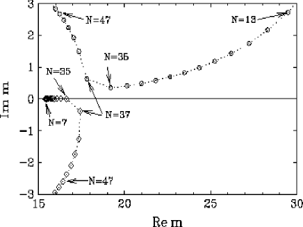
Figure 1: Trajectories of the effective channel labels $m_{\rm eff}(N)$ in the complex $m$-plane for laser frequency $\omega=0.0043$a.u., intensity $I$ = 10¹¹ W/cm² and varying harmonic order $N$ for HHG by H^- ion. Positions of two effective channel labels for odd integer $N$ are denoted respectively by circles and diamonds.

It can be demonstrated that large ${\rm Im}(m_{\rm eff})$ lead to suppression of the HHG process. Therefore the critical $N_{c}$ marks the beginning of the cutoff region for HHG. As shown in Ref. [10], approximate analytical solution of Eqs. (17), (16), (18) shows that the critical value $N_{c}$ is equal to

$$N_{c}\,\omega=|E_{a}|+3.1731\,U_{p}~{},$$ (20)

in agreement with the well known result of Refs. [3, 4, 8, 22].

In order to find simple physical interpretation for the effective channels, let us note that Eqs. (16), (17), (18) may be considered as classical equations of motion in the laser field. They define the classical trajectories along which the electron first goes away from the atom, and then returns back accumulating during this motion energy from the laser field that is necessary for HG. This physical picture agrees with the atomic antenna concept discussed in Section 1. It also comes in line with the Corcum model [2] based entirely on the classical trajectories. Even more close relation can be found with the approach of Lewenstein et al [8], which uses the saddle point method to integrate over the momenta ${\bf p}$ in formula (4).

Eqs. (6) and (19) provide two different ways to describe the atomic antenna concept, either in terms of real physical channels in the intermediate ATI spectrum, or by using the effective channels for the intermediate state. Each approach has its advantages which can be beneficial for different aspects of HHG problem. Importantly, the above discussion ensures identity of the two formulas since (19) was derived directly from (6).

4 Photoionization and recombination

Eq. (6) shows that the process of HHG is intimately related to ionization and LAR. This fact makes the latter processes very interesting from the perspective of the atomic antenna concept, in addition to their well known importance as the basic events in the laser-matter interaction. This Section describes the recent progress in the theory of these two ”elementary” phenomena.

   

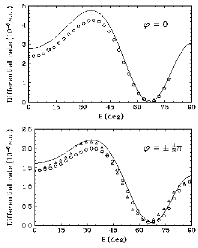
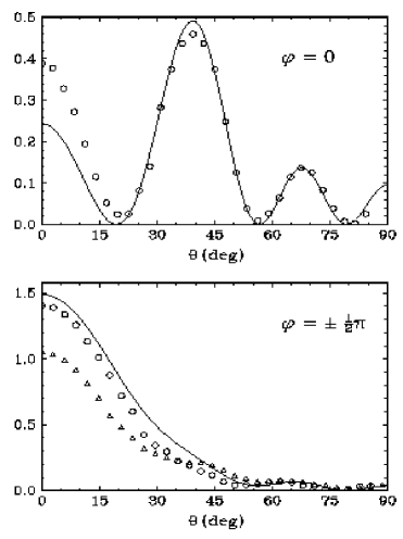
Figure 2: Detachment of H^- ion in bichromatic field with the frequencies $\omega=0.0043$ a.u. and $3\omega$ and intensities $I_{1}=10^{10}{\rm W}/{\rm cm}^{2}$ and $I_{2}=10^{9}{\rm W}/{\rm cm}^{2}$ respectively. Differential detachment rate (in units $10^{-8}$a.u.) as a function of the electron emission angle $\theta$ is shown for various values of the field phase difference $\varphi$ as indicated in the plots. Open symbols show results of calculations of [19] (in the $\varphi=\pm\frac{1}{2}\pi$ plot the open circles show the results for $\varphi=\frac{1}{2}\pi$ and open triangles these for $\varphi=-\frac{1}{2}\pi$). Solid curves show results of the adiabatic theory [18] (which coincide for $\varphi=\frac{1}{2}\pi$ and $\varphi=-\frac{1}{2}\pi$). Left - the first ATD peak, corresponding to absorption of $n=8$ photons of frequency $\omega$. Right - the third ATD peak, corresponding to absorption of $n=10$ photons of frequency $\omega$.

Consider first the multiphoton ionization. Adopting the Keldysh-type approach which neglects the field of the atomic core in the final state one can present the amplitude of the ionization in the following form

$$A_{m}({\bf p}_{m})=\frac{1}{T}\int_{0}^{T}\langle\phi_{{\bf p}_{m}}(t)\,|\,V(t)\,|\,\phi_{a}(t)\rangle~{},$$ (21)

where $\phi_{\bf p}(t)=\phi_{\bf p}({\bf r},t)$ is the Volkov wave function (5) and ${\bf p}_{m}$ satisfies the energy conservation law

$$E_{a}+m\,\omega=\frac{1}{2}\,{\bf p}_{m}^{2}+U_{p}~{}.$$ (22)

Fast variation of the phase of the integrand in (21) allows one to use the saddle-point approach for integration over the time $t$. This approximation, first proposed by Keldysh [11], was developed in detail in Refs. [12, 13, 14]. Using this scheme one presents the photoionization amplitude as

$$A_{m}({\bf p}_{m})=\sum_{\mu}A_{m\mu}({\bf p}_{m})~{},$$ (23)

where summation runs over essential saddle points labeled by subscript $\mu$. Note that in Eq. (6), relating the ionization problem with HG, it is sufficient to take into account the amplitude which arises from only one saddle point (of two) labeled as $\mu_{0}$; another saddle point gives the same contribution that produces a factor 2.

The technique described above was refined in Refs. [15, 16]. In the pioneer publications [11, 12, 13, 14] the momentum $p$ of the ionized electron was treated as a small quantity, and all essential functions were expanded in powers of $p/\kappa$. This approximation restricted the applicability of the approach, since for high channels in ATI spectrum the momentum is not small. Refs. [15, 16] demonstrated that the technique can be modified to include large electron momenta as well. Importantly, this modification retains simplicity and clear physical nature of the Keldysh approach.

One can anticipate that the Keldysh-type methods should produce reliable results for photodetachment of negative ions, where the detached electron is influenced negligibly by the Coulomb field of the residual atomic particle. Due to this reason the photodetachment was in the focus of attention of Refs. [15, 16] which compared the results of improved Keldysh approximation with a variety of numerical and experimental data available for negative ions. Refs. [17, 18] continued this study and extended it to the case of the two-color laser field. Detailed description of all results obtained in these works would bring us too far away from the main topic of this paper. However, it is important to mention that the overall accuracy of the modified Keldysh approximation proves be very high. It closely reproduces results of other, much more sophisticated methods for total probabilities of detachment as well as for spectral and angular distributions of photoelectrons both for the weak and strong field regimes (i.e., for any value of the Keldysh parameter $\gamma=\kappa\omega/F$). An example of photodetachment of the H^- in bichromatic laser field with the frequencies $\omega=0.0043$ a.u. and $3\omega$ shown in Fig. 2 illustrates this point.

Let us now turn our attention to the other relevant problem, laser-assisted photo recombination (LAR). Consider the electron-atom impact in a laser field which results in creation of a negative ion and HG. Since the system can acquire energy from the laser field due to absorption of several laser quanta, the emitted harmonics should exhibit the equidistant spectral distribution. Strange enough, this important process was not studied theoretically until two recent almost simultaneous publications [20, 21].

The amplitude of the photorecombination can be written as

$$C_{m}({\bf p})=\frac{1}{T}\int_{0}^{T}\langle\phi_{a}(t)\,|\exp(i\Omega t)\,U\,|\phi_{\bf p}(t)\rangle~{}.$$ (24)

Here $U=\mbox{\boldmath$\epsilon$}\cdot{\bf r}$ describes the potential which is responsible for the harmonic production, and $\Omega$ is the energy of the generated harmonic which satisfies the energy conservation constraint

$$\Omega=\frac{{\bf p}^{2}}{2}+U_{p}+|E_{a}|+m\,\omega~{},$$ (25)

in which $m$ is the number of laser photons absorbed during recombination. The wave function of the electron in the continuum in Eq. (24) can be described by the Volkov wave function, similarly to the Keldysh-type approach to photoionization. Comparing the amplitudes (24) and (21) one observes their close similarity. This fact allows one to develop the theory on the basis of formula (24) along the lines described above for the ionization problem. In particular, one can use the saddle-point approximation for integration over the time variable in (24).

This approach, suggested in Ref. [20], is supplemented in the cited paper by several numerical examples. One of them, shown in Fig. 3, depicts the cross section of recombination on hydrogen atom in a laser field with $\omega=0.0043$ a.u. and the intensity $I=10^{11}$ W/cm² versus the energy of the emitted high harmonic.

                      

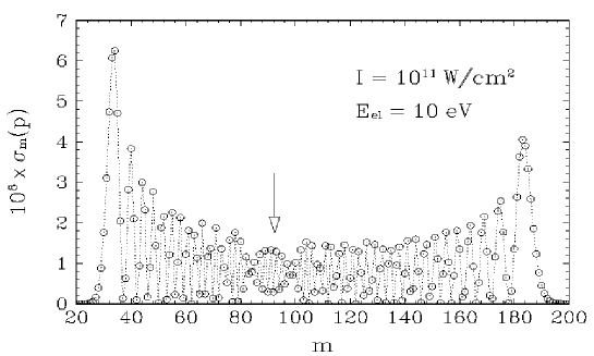
Figure 3: Cross section $\sigma_{m}(p)$ for laser-assisted recombination of the electron with the energy $E_{\rm el}=10$ eV into the bound state in H^- ion [20]. The results are shown for the laser field with the frequency $\omega=0.0043$ a.u. and the intensity $I=10^{11}$ W/cm². The symbols are joined by lines to help the eye.

Since this is the first work in the field we could not compare our results with other calculations. Bearing in mind that the recombination process has similarities with the ionization problem, where similar approach works well one can expect reliable results in the recombination problem as well.

5 Quantitative illustrations for HHG

To illustrate the applicability of the two methods, the factorization technique and the method of effective channels, consider an example of HHG by hydrogen negative ion in a laser field with $\omega=0.0043$ a.u. . Using the factorization procedure one needs first to calculate the amplitudes of ATI and LAR, which can be done by the technique discussed in Sections 4. After that employing (6) one finds the amplitude of HHG, and from (11) the HHG rates. The results are presented in Fig. 4.

It is important to note a strong interference of contributions coming from different intermediate channels $m$. In the plateau region it is responsible for an oscillatory pattern, and becomes even more important in the cutoff region, where a contribution of any single channel drastically exceeds the results of an accurate summation over a large number of channels.

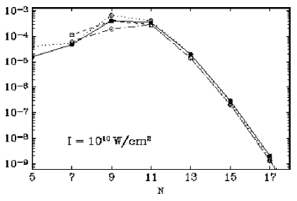
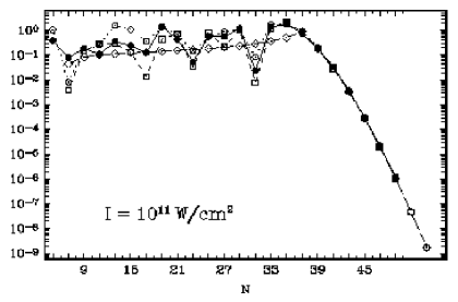
Figure 4: Harmonic generation rates (11) (in sec^-1) for H^- ion in the laser field with the frequency $\omega=0.0043$ a.u. and various values of intensity $I$ as indicated in the plots. Closed circles - results obtained by Becker et al [22], open circles - calculations [6, 7] based on factorization procedure and performing numerical summation (6) over contributions of different ATI channels, open diamonds – calculations of Ref. [20] based on the effective channels approach (19) with a single effective channel $m_{\rm eff}(N)$ taken into account (namely, the effective channels shown by diamonds in Fig. 1); open squares – same but taking into account two saddle points $m_{c}(N)$ (namely, the effective channels shown by diamonds and circles in Fig. 1). The symbols are joined by lines to help the eye.

In order to apply the technique based on the effective channels one needs to calculate the ”elementary” amplitudes for the complex-valued number $m_{\rm eff}$ of quanta absorbed on the first step of three-step process. This can be done by the approach described in Section 3, because it relies on analytical methods for calculation of these amplitudes that remain valid for a complex-valued $m$. Taking the effective channels (presented in Fig. 1 for $I$ = 10¹¹ W/cm²), calculating for them the ”elementary” amplitudes and applying formula (19), we find the rates presented in Fig. 4. If one takes into account in the summation (19) over $m_{\rm eff}$ a single effective channel, shown by diamonds in Fig. 1, then the cutoff region is nicely described, as well as the overall pattern in the plateau domain. However such one-saddle-point approximation does not reproduce structures in the $N$-dependence of HG rates. Taking into account the two effective channels, shown by diamonds and circles in Fig. 1 improves the results for the rates in the plateau domain by producing appropriate structures in the $N$-dependence. Remarkably, this two-saddle-point calculation gives correct positions of minima and maxima in the rate $N$-dependence, albeit the magnitudes of the rate variation is reproduced somewhat worse; for instance the depth of the minimum at $N=17$ is quite strongly overestimated.

Fig. 4 shows good agreement of the approaches based on the factorization technique and on the effective channels, which both are in accord with the results of Ref. [22]. This agreement holds both for multiphoton regime (left part of Fig. 4), as well as in the tunneling regime (right part of Fig. 4).

6 Above-Threshold Ionization in high channels

The methods discussed in Sections 2, 3 can be applied to a number of other multiphoton problems. To illustrate this point consider the factorization technique for ATI. The ionization amplitude $A_{n}({\bf p}_{n})$ in the Keldysh-type approximation, considered in (21), neglects interaction of the released electron with the core. Let $A^{(1)}_{n}({\bf p}_{n})$ be a correction that takes this interaction into account. In this notation the total amplitude of ATI with absorption of $n$ photons is $A^{\rm tot}_{n}({\bf p}_{n})=A_{n}({\bf p}_{n})+A^{(1)}_{n}({\bf p}_{n})$. Using the approach of Ref. [5] we find the following relation

$$A^{(1)}_{n}({\bf p}_{n})=\sum_{m}\sum_{\mu}\sum_{\sigma=\pm 1}A_{m}(\sigma{\bf K_{m}})\frac{1}{R_{m\mu}}f^{B}({\bf p}_{n},\sigma{\bf K}_{m})~{},$$ (26)

which presents the sufficiently complicated correction $A^{(1)}_{n}({\bf p}_{n})$ in terms of two ”elementary” amplitudes $A_{m}({\bf K}_{m})$ and $f^{B}({\bf p},{\bf K})$. The later one describes the electron-atom impact in the laser field in the Born approximation. This scattering can be named quasielastic, since the atom remains in the same state, but the electron momentum is changed ${\bf K}\rightarrow{\bf p}$ both in direction and absolute value. Summation over $\mu$ in formula (26) reflects the fact that the electron emission into the continuum takes place at two moments of time $t_{m\mu}$ ($\mu=1,\,2$) per laser period. The electron return to the atom is ensured only if the electron momentum is parallel (for one value of $\mu$) or antiparallel (for another $\mu$) to the field, see details in Ref. [5]. This fact is taken into account by a summation index $\sigma=\pm 1$ in (26).

Eq. (26) is obtained via application of the factorization technique to ATI. It has a transparent physical meaning. Ionization with absorption of $n$ photons needs that first $m$ quanta are absorbed by an atom removing the electron from an atom into the continuum state with momentum $\pm{\bf K}_{m}$. The collision of this electron with the atom (often referred to as rescattering) results in absorption of additional $n-m$ quanta and transition of the electron into a state with momentum ${\bf p}_{n}$. All intermediate ATI channels labeled by index $m$ contribute coherently. This physical picture of ATI agrees with the atomic antenna concept, as was first discussed in [1].

We applied (26) to calculation of Above Threshold Detachment (ATD) from H^- ion. Fig. 5 shows the results which clearly indicate that the contribution of the process (26) to the angular distributions of ATD spectra is dominating for higher ATD channels while for low channels rescattering effects are small .

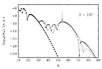
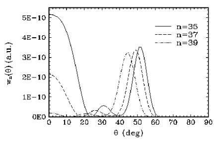
Figure 5: Differential above-threshold detachment rates $w_{n}(\theta)$. Left - the rates versus the number $n$ of absorbed photons for fixed value of electron ejection angle $\theta$. Right - same as functions of $\theta$ for fixed $n$. An H^- ion is irradiated by the laser wave with frequency $\omega=0.0043$ a.u. and intensity $I=5\times 10^{10}$W/cm². The minimum number of photons necessary for ionization is $n_{\rm min}=11$. Curves - present calculation with account of rescattering; closed circles - Keldysh-type approximation of [15]. The arrow indicates the plateau cutoff as predicted by classical theory [24].

7 Eikonal approach to the Coulomb field

The Keldysh-type approximation for laser induced ionization, as described in Section 4, discards interaction of receding photoelectrons with the atomic core. The most significant part of this interaction arises due to the Coulomb field of the core. That is why a number of numerical applications considered above is carried out for negative ions, where the core is neutral. However, for the multiphoton processes with neutral atoms, the Coulomb forces between the active electron and the residual positive ion become operative. This interaction was taken into account first in Ref. [12] in the quasistatic limit of the small Keldysh parameter $\gamma=\kappa\omega/F\ll 1$. A very simple relation was obtained between the photoionization rate $w_{C}$ for the electron bound by a potential with the Coulomb field produced by a core charge $Z$ and its counterpart $w_{\rm sr}$ for the electron with the same binding energy $\kappa^{2}/2$ but bound by short range forces:

$$w_{C}=\left(\frac{2\kappa^{2}}{F}\right)^{2Z/\kappa}w_{\rm sr}~{}.$$ (27)

This result means that for conventional conditions the presence of the Coulomb field enhances the rates by several orders of magnitude. It is remarkable that the relation (27) holds in fact for arbitrary value of the Keldysh parameter, both in the multiphoton and tunneling region, as was established in a more elaborate theory by Perelomov and Popov [14]. This result agrees well with experimental data for the total rates [23].

The theory of Perelomov and Popov is restricted to ejection of low-energy electrons. It is usually anticipated that these electrons give principal contribution to the total rates summed over all ATI channels as well as over ejection angles. The current experiments, however, are able to select an individual ATI channel even for a large number of absorbed quanta. Both energy and angular distributions of these electrons manifest some fascinating features which are the object of interest in modern experiment and theory. This fact prompts to develop a theory which, reproducing the Perelomov-Popov results for low electron energy, could also describe high-energy photoelectrons. The antenna-type phenomena considered in this paper provide an additional inspiration for this study. The ionization amplitude in Eqs. (6), (26) should be summed over the number $m$ of quanta absorbed that should be large enough. This makes the electron momentum in the intermediate ATI channels to be also large. Therefore we need to know how the Coulomb field affects the amplitudes for large momenta.

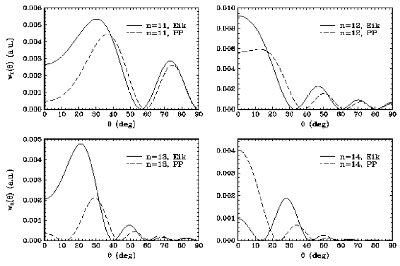
Figure 6: Angle-resolved photoionization rates $w_{n}(\theta)$ for four lowest open ATI channels labeled by a number of absorbed photons $n$ ($n=11$ corresponds to the lowest open ATI channel). Hydrogen atom is illuminated by the laser wave with frequency $\omega=2$ eV and intensity $I=10^{14}$W/cm²; solid curves - eikonal theory, dashed curves - the Perelomov-Popov theory [14] (27).

In order to address this issue we develop the eikonal approach for this problem. It presents a simplified version of the semiclassical approximation, that assumes that the Coulomb field does not produce significant distortions of classical trajectories describing electron propagation in the continuum (i.e., the electron wiggling motion in the laser field). The Coulomb field comes into the picture through its contribution to the action $\int^{t}(Z/r)dt$ calculated along the classical trajectories discussed. Within the semiclassical approximation the action plays a role of the wave function phase. It is important that the Coulomb field can produce large contribution to the action while its distortion of the trajectories can remain unsubstantial Calculating the action, one is able to construct the semiclassical wave function for the released electron, and find with its help the ionization amplitude. If we totally neglect in this scheme the Coulomb field putting $Z=0$, the eikonal wave function simplifies to be the Volkov function, and we return to the Keldysh-type approximation. An important verification of our eikonal approach provides the limit of low photoelectron energy where we reproduce the Perelomov-Popov result (27). Fig. 6 presents a quantitative example which illustrates importance of the Coulomb interaction.

8 Conclusions

Atomic antenna gives a clear physical idea how the complicated multiphoton processes are operative. Absorption of large number of quanta from the laser field needs that one of the atomic electrons is at first released from an atom. After that, propagating in the core vicinity, the electron accumulates high energy from the laser field and, returning to the atomic core, transfers this energy into other channels such as HHG, ATI or others. Importantly, this physical picture is implemented in a simple and reliable formalism. We discussed two convenient ways to present the theory. One of them, called the factorization technique, is presented by Eqs. (6), (26) for the cases of HHG and ATI. In this approach the amplitude of a complicated process is expressed via the physical amplitudes of more simple, ”elementary” processes. Another scheme, called the effective channels method, is based on Eq. (19) for HHG. The effective channels are closely related to the classical trajectories, that makes them convenient for qualitative, as well as numerical studies. We demonstrated an equivalence of the two approaches.

Applications of both formalisms need calculation of the ”elementary” amplitudes. This can be achieved by using the modified Keldysh-type approach which very accurately reproduces data for photodetachment, and, hopefully, for recombination and electron-atom scattering in the laser field as well. The Coulomb field of the atomic core can be taken into account within eikonal approximation. Reliability of the theoretical approaches is demonstrated by quantitative applications.

References

- [1] M. Yu. Kuchiev, Pis’ma Zh. Eksp. Teor. Fiz. 45, 319 (1987) [JETP Letters 45, 404 (1987)].
- [2] P. B. Corkum, Phys. Rev. Lett. 71, 1994 (1993).
- [3] J. L. Krause, K. J. Schafer, and K. C. Kulander, Phys. Rev. Lett. 68, 3535 (1992).
- [4] K. C. Kulander, K. J. Schafer, and J. L. Krause, in Super-Intense Laser-Atom Physics, Vol. 316 of NATO Advanced Study Institute, Series B: Physics, edited by B. Piraux et al (Plenum, New York, 1993), p. 95.
- [5] M. Yu. Kuchiev, J. Phys. B 28, 5093 (1995).
- [6] M. Yu. Kuchiev and V. N. Ostrovsky, J. Phys. B 32, L189 (1999).
- [7] M. Yu. Kuchiev and V. N. Ostrovsky, Phys. Rev. A 60, 3111 (1999).
- [8] M. Lewenstein, Ph. Balcou, M. Yu. Ivanov, A. L’Huillier, and P. B. Corkum, Phys. Rev. A 49, 2117 (1994).
- [9] M. Lewenstein, P. Sallièrs, and A. L’Huillier, Phys. Rev. A 52, 4747 (1995).
- [10] M. Yu. Kuchiev and V. N. Ostrovsky, http://xxx.lanl.gov/physics/0007016.
- [11] L. V. Keldysh, Zh.Éksp.Teor.Fiz.47, 1945 (1964) [Sov.Phys.JETP 20, 1307 (1965)].
- [12] A. M. Perelomov, V. S. Popov, and M. V. Terent’ev, Zh. Éksp. Teor. Fiz. 50, 1393 (1966) [Sov. Phys.-JETP 23, 924 (1966)].
- [13] A. M. Perelomov, V. S. Popov, and M. V. Terent’ev, Zh. Éksp. Teor. Fiz. 51, 309 (1966) [Sov. Phys.-JETP 24, 207 (1967)].
- [14] A. M. Perelomov and V. S. Popov, Zh. Éksp. Teor. Fiz. 52, 514 (1967) [Sov. Phys.-JETP 25, 336 (1967)].
- [15] G. F. Gribakin, M. Yu. Kuchiev, Phys. Rev. A 55, 3760 (1997).
- [16] G. F. Gribakin, M. Yu. Kuchiev, J. Phys. B 30, L657 (1997).
- [17] M. Yu. Kuchiev and V. N. Ostrovsky, J. Phys. B 31, 2525 (1998).
- [18] M. Yu. Kuchiev and V. N. Ostrovsky, Phys. Rev. A 59, 2844 (1999).
- [19] D. A. Telnov, J. Wang, and S. I. Chu, Phys. Rev. A 51, 4797 (1995).
- [20] M. Yu. Kuchiev and V. N. Ostrovsky, Phys. Rev. A 61, 033414 (2000).
- [21] A. Jaroń, J. Z. Kamińsky, and F. Ehlotzky, Phys. Rev. A 61, 023404 (2000).
- [22] W. Becker, S. Long, and J. K. McIver, Phys. Rev. A 50, 1540 (1994).
- [23] S. F. J. Larochelle, A. Talebpour, and S. L. Chin, J. Phys. B 31, 1215 (1998).
- [24] G. G. Paulus, W. Becker, W. Nicklich, and H. Walter, J. Phys. B 27, L703 (1994).