Passive Tracer Dynamics in 4 Point-Vortex Flow

Abstract

The advection of passive tracers in a system of 4 identical point vortices is studied when the motion of the vortices is chaotic. The phenomenon of vortex-pairing has been observed and statistics of the pairing time is computed. The distribution exhibits a power-law tail with exponent $\sim 3.6$ implying finite average pairing time. This exponents is in agreement with its computed analytical estimate of $3.5$. Tracer motion is studied for a chosen initial condition of the vortex system. Accessible phase space is investigated. The size of the cores around the vortices is well approximated by the minimum inter-vortex distance and stickiness to these cores is observed. We investigate the origin of stickiness which we link to the phenomenon of vortex pairing and jumps of tracers between cores. Motion within the core is considered and fluctuations are shown to scale with tracer-vortex distance $r$ as $r^{6}$. No outward or inward diffusion of tracers are observed. This investigation allows the separation of the accessible phase space in four distinct regions, each with its own specific properties: the region within the cores, the reunion of the periphery of all cores, the region where vortex motion is restricted and finally the far-field region. We speculate that the stickiness to the cores induced by vortex-pairings influences the long-time behavior of tracers and their anomalous diffusion.

1 Introduction

The understanding of the motion of a passive tracer evolving in an unsteady incompressible flow is fundamental due to its numerous applications in various fields of research. They range from pure mathematical interest to geophysical flows or chemical physics. The underlying problem is related to the Lagrangian representation of the fluid evolution. This approach uncovered the phenomenon of chaotic advection Aref84 -Crisanti92 , which refers to the chaotic nature of Lagrangian trajectories in a non chaotic velocity field and hence reflects a non-intuitive interplay between the Eulerian and Lagrangian perspective. The ongoing interest in geophysical flows sustains interest in two-dimensional models provenzale99 -Meleshko93 . In case of an incompressible flow, the tracer’s motion can be described by a non-autonomous Hamiltonian. Another peculiarity of two-dimensional turbulent flows is the presence of the inverse energy cascade, which results in the emergence of coherent vortices, dominating the flow dynamics Benzi86 -Carnevale91 . In order to tackle these problems, point vortices have been used with some success to approximate the dynamics of finite-sized vortices Zabusky82 -VFuentes96 , as for instance in punctuated Hamiltonian models Carnevale91 ,Benzi92 ; Weiss99 . Recent work shows that high-dimensional point vortex systems have both the features of extremely high-dimensional as well as low-dimensional systems Weiss98 ; moreover, the merging processes observed in decaying two-dimensional turbulence have been shown to result from the interaction of a few number of close vortices Zabusky96 and make the understanding of low dimensional vortex dynamics an essential ingredient of the whole picture Aref99 ; Sire2000 .

Another aspect of the problem is related to transport properties, which for various observations and models exhibit anomalous features. These anomalous properties are linked to Levy-type processes and their generalizations Chernikov90 -Kovalyov2000 . These properties are often related to the presence of coherent structures, which can be identified from a Lagrangian perspective by the means of an analytic criterionHaller2000 . In previous work, the advection in systems of three point vortices evolving on the plane has been extensively investigated KZ98 -LKZpreprint . Three point-vortex systems on the plane have the advantage of being an integrable system and often generate periodic flows (in co-rotating reference frame)Aref79 -Tavantzis88 . This last property allows the use of Poincaré maps to investigate the phase space of passive tracers whose motion belongs to the class of Hamiltonian systems of $1-1/2$ degree of freedom. A well-defined stochastic sea filled with various islands of regular motion is observed and among these are special islands also known as “vortex cores” surrounding each of the three vortices. Transport in these systems is found to be anomalous, and the exponent characterizing the second moment exhibit a universal value close to 3/2, in agreement with an analysis involving fractional kinetics LKZpreprint . In this light, the origin of the anomalous properties and its multi-fractal nature is clearly linked to the existence of islands within the stochastic sea and the phenomenon of stickiness observed around them KZ2000 ; LKZpreprint . Nevertheless the inherent periodic nature of the motion of three vortices may be thought as artificial when considering systems with more degree of freedom and therefore universal long time behavior of transport properties may be considered as particular to these low-dimensional periodic systems.

The motion of $N$ point vortices on the plane is generically chaotic for $N\geq 4$ Novikov78 -Ziglin80 . However, a system of four vortices remains a low dimensional system, but loses the periodic property of three point-vortex systems and is in this sense a more realistic modelization of observed low dimensional behavior. The chaotization of the underlying flow is expected to bring modifications to the transport properties studied in KZ98 -LKZpreprint ; the nature and relevance of the changes is although unknown. A precise study of these questions is required and the answer consequently provides a way to test the robustness of the results obtained with three vortices.

In this paper we investigate numerically the motion of a passive tracer in the field generated by four identical point vortices on the plane. This study follows previous work found in Ref. Babiano94 and Boatto99 . In Ref. Babiano94 , a first physical picture was given and the persistence of vortex cores where tracers are trapped was clearly stated, while in Ref. Boatto99 a rich extensive study is presented and emphasis is made on the quasi-regular motion of tracers in the region far from the vortices. We note that in both of these papers, the characterization of “regular” trajectories is defined by the means of vanishing Lyapunov exponents. For instance, when a tracer is trapped within cores, despite the core’s chaotic motion, two nearby initial conditions do not diverge exponentially. The goal of the present work is to identify the different structures and different mechanisms which may influence the transport properties of passive particles. Since parameter space is quite large, the philosophy is essentially descriptive, and tracers motion are studied for one arbitrary chosen initial condition of the vortex system. As the far field region has been investigated Boatto99 , we focus on the motion near or inside the cores, which we believe should be generic even for many vortex systems. We will come to the issue of transport properties and finite-time Lyapunov exponents in a forthcoming publication.

In Sec. 2, we describe briefly the motion of four vortices. We present a Poincaré section of the vortex system, which provides a good test to our numerical integration and allows to characterize easily the chaotic or non chaotic nature of the motion. A new section capturing all equivalent physical realizations of the flow is introduced. This section shows the existence of non-uniformity in the phase space, which is linked to the permutation of vortices and is related to the observation of vortex-pairing. Statistics on pairing times are computed and exhibit power-law tails, implying finite average pairing time. In Sec. 3 the motion of tracers is studied, the presence of cores is confirmed and stickiness to the vortex cores is observed. The influence of vortex pairing is studied, which proves to be a good trapping (untrapping) mechanism of tracers around the cores. Pairing of vortices allows a special behavior of tracers jumping from one core to another core, which opens the possibility in many vortex systems of special transport features resulting from jumps between cores. The motion within the core is studied, dependence of fluctuations as a function from the distance to the vortex are computed, and no typical diffusion behavior is found.

2 Vortex motion

2.1 Definitions

The solution of the two-dimensional Euler equation, describing the dynamics of a singular distribution of vorticity

$$\omega(z)=\sum_{\alpha=1}^{N}k_{\alpha}\delta\left(z-z_{\alpha}(t)\right),$$ (1)

where $z$ locates a position in the complex plane, $z_{\alpha}=x_{\alpha}+iy_{\alpha}$ is the complex coordinate of the vortex $\alpha$, and $k_{\alpha}$ its strength, in an ideal incompressible two-dimensional fluid can be described by a Hamiltonian system of $N$ interacting particles (see for instance Lamb45 ), referred to as a system of $N$ point vortices. The system’s evolution writes

$$k_{\alpha}\dot{z}_{\alpha}=-2i\frac{\partial H}{\partial\bar{z}_{\alpha}}\>,\hskip 28.45274pt\dot{\bar{z}}_{\alpha}=2i\frac{\partial H}{\partial(k_{\alpha}z_{\alpha})}\>,(\alpha=1,\cdots,N)\>,$$ (2)

where the couple $(k_{\alpha}z_{\alpha},\bar{z}_{\alpha})$ are the conjugate variables of the Hamiltonian $H$. The nature of the interaction depends on the geometry of the domain occupied by the fluid, for the case of an unbounded plane, the resulting complex velocity field $v(z,t)$ at position $z$ and time $t$ given by the sum of the individual vortex contributions, writes:

$$v(z,t)=\frac{1}{2\pi i}\sum_{\alpha=1}^{N}k_{\alpha}\frac{1}{\bar{z}-\bar{z}_{\alpha}(t)}.$$ (3)

and the Hamiltonian becomes

$$H=-\frac{1}{2\pi}\sum_{\alpha>\beta}k_{\alpha}k_{\beta}\ln|z_{\alpha}-z_{\beta}|=-\frac{1}{4\pi}\ln\Lambda\>.$$ (4)

The translational and rotational invariance of $H$, provides the motion equations (2) three other conserved quantities besides the energy,

$$Q+iP=\sum^{N}_{\alpha=1}k_{\alpha}z_{\alpha},\hskip 34.14322ptL^{2}=\sum_{\alpha=1}^{N}k_{\alpha}|z_{\alpha}|^{2}.$$ (5)

Among the different constants of motion, there are three independent first integrals in involution: $H$, $Q^{2}+P^{2}$ and $L^{2}$, consequently the motion of three vortices on the plane is always integrable and chaos arises when $N\geq 4$.

2.2 Canonical Transformations

Due to the chaotic nature of 4-point vortex system, the understanding of vortex motion necessitates a different approach than for integrable 3-vortex systems. We follow Ref. ArefPomp82 and perform a canonical transformation of the vortex coordinates. This transformation results in an effective system with $2$ degrees of freedom, providing a conceptually easier framework, best suited for a detailed analysis of the motion of four identical vortices. For instance, this transformation allows to perform well defined two-dimensional Poincaré sections, from which the properties of the motion are analyzed. The details of the transformation are not given here but the outline is the following, using $z_{\alpha}$ ($\alpha=1,\cdots,4$) as the complex coordinates of the four vortices.

$$(2J_{n})^{\frac{1}{2}}e^{i\theta_{n}}=N^{-\frac{1}{2}}\sum^{N}_{\alpha=1}\exp(i(2\pi n/N)(\alpha-1))z_{\alpha}\>,\hskip 28.45274ptn=0,\cdots,N-1\>,$$ (6)

with new canonical variables

$$\left\{\begin{array}[]{ccc}\phi_{1}=\frac{1}{2}(\theta_{1}-\theta_{3}),&\phi_{2}=\frac{1}{2}(\theta_{1}+\theta_{3})-\theta_{2},&\phi_{3}=\theta_{2}\\ I_{1}=J_{1}-J_{3},&I_{2}=J_{1}+J_{2},&I_{3}=J_{1}+J_{2}+J_{3}\>.\end{array}\right.$$ (7)

The resulting Hamiltonian is rather complicated but independent of $\phi_{3}$, meaning that $I_{3}=\frac{1}{2}L^{2}$ is a constant of motion. We mention that this transformation by preserving and making use of the constants of motion is taking into account the continuous symmetries of the system. However, besides these symmetries, the system is also invariant under the discrete group of permutations. This last feature is particular to the situation of four identical vortices. It has been shown that for a subgroup of these permutation, the effect of these symmetries on the couple $(I_{1},\phi_{1})$ leads to simple linear transformations ( see ArefPomp82 , results are reproduced in Table 1), but the effect of for instance the permutation $(2,1,3,4)$ on the vortex system (which can be thought of as a relabeling $z^{\prime}_{1}=z_{2}$, $z^{\prime}_{2}=z_{1}$, $z^{\prime}_{3}=z_{3}$, $z^{\prime}_{4}=z_{4}$), leads to no simple transformation on $(I_{1},\phi_{1})$. The effect of these permutations on $(I_{2},\phi_{2})$ does neither lead to simple transformations. We shall discuss some consequences of these issues in the computation of Poincaré sections.

permutation	$I_{1}$	$\phi_{1}$
$(1,2,3,4)$	$I_{1}$	$\phi_{1}$
$(4,1,2,3)$	$I_{1}$	$\phi_{1}-\pi/2$
$(2,3,4,1)$	$I_{1}$	$\phi_{1}+\pi/2$
$(2,1,4,3)$	$-I_{1}$	$-\phi_{1}+\pi/2$
$(3,4,1,2)$	$I_{1}$	$\phi_{1}$
$(4,3,2,1)$	$-I_{1}$	$-\phi_{1}-\pi/2$
$(3,2,1,4)$	$-I_{1}$	$-\phi_{1}$
$(1,4,3,2)$	$-I_{1}$	$-\phi_{1}$

Table 1: Effect of the subgroup $D_{4}$ on the values of $(I_{1},\phi_{1})$.

To summarize the results obtained in ArefPomp82 , the motion is in general chaotic, except for some special initial conditions, for instance when the vortices are forming a square the motion is periodic and the vortices rotate on a circle, then symmetric deformation ($z_{3}=-z_{1}$ and $z_{4}=-z_{2}$) of the square lead to quasiperiodic motion (periodic motion in a given rotating frame), see ArefPomp82 for the complete details.

2.3 Poincaré sections

As a prerequisite to our investigations on the passive tracer’s motion, a basic understanding of the vortex subsystem behavior is necessary. For this matter, an arbitrary initial condition is chosen and a Poincaré section of the vortex system is computed. The section is a tool which insures that for the considered initial condition, the trajectory has the desired generic chaotic behavior. To perform Poincaré sections of the system, we proceed as in ArefPomp82 , and use the set of canonical conjugated variables:

$$\left\{\begin{array}[]{cc}R_{1}=\left(I_{1}+I_{3}\right)^{\frac{1}{2}}\cos 2\phi_{1}&R_{2}=\left(I_{3}-I_{2}\right)^{\frac{1}{2}}\sin 2\phi_{2}\\ P_{1}=\left(I_{1}+I_{3}\right)^{\frac{1}{2}}\sin 2\phi_{1}&P_{2}=\left(I_{3}-I_{2}\right)^{\frac{1}{2}}\cos 2\phi_{2}\end{array}\right.\>,$$ (8)

to compute the section $R_{2}=0$, $\dot{R}_{2}<0$.

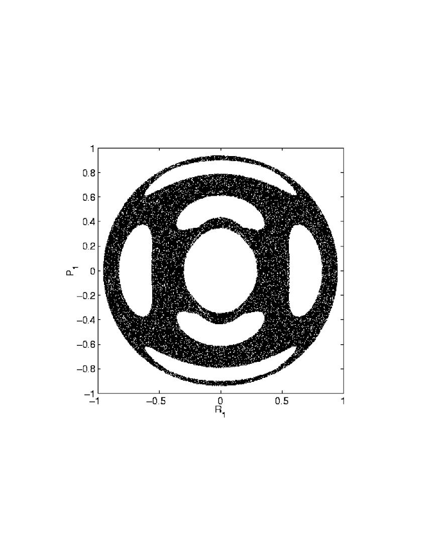
Figure 1: Poincaré section of the four vortex system in the chaotic regime for a given initial condition. The section is computed using the variables of the reduced system (8). The conditions imposed are the following: $R_{2}=0$, $\dot{R}_{2}<0$.

The result of this section for the arbitrary chosen initial condition is presented in Fig. 1. We notice that the section reproduces relatively well the results obtained in PullSaff91 , where the section was computed using a numerical integration of the reduced system. This has the advantage of offering a natural test of the accuracy of our numerical integration, which is made in our case in the original vortex complex variables using a fifth order simplectic Gauss-Legendre scheme McLachlan92 . Previous analogous sections can be seen in ArefPomp82 and PullSaff91 and are all in good agreement with our result. The motion of the vortices is chaotic. This settles the choice of the initial condition of the vortex system, which we will use from now on.

We notice that Fig.1 has symmetries which relate to the effect of the permutations illustrated in Table 1. This somehow reflects, as anticipated earlier on, that to equivalent physical configurations of the vortex system correspond different points located in different regions of the section. Moreover the fact that the new canonical variables are not invariant under all permutation of the vortices implies that equivalent physical realizations of the system have different location in the reduced phase space, and are likely to not all belong to the section. From the advection point of view, equivalent physical configurations generate identical flows, so the proposed section may not be best suited for investigating advection and possible patterns. However they prove very useful to characterize the type of motion (periodic, quasiperiodic, chaotic). One possible way to circumvent this location problem follows from noticing that the condition $R_{1}=0$ or $P_{1}=0$ remains unchanged by the permutations listed in Table 1, and to capture all equivalent systems, we can superimpose the two following sections $R_{1}=0$, $\dot{R}_{1}<0$, and $R^{\prime}_{1}=0$, $\dot{R}^{\prime}_{1}<0$, where ^′ stands for the values of $R_{1}$ and $\dot{R}_{1}$ obtained after the relabeling $(2,1,3,4)$ is performed; (note that the superimposition does not modify the obtained section for the considered initial condition, but allows for more points and reduces computation times). The corresponding section is plotted in Fig. 2, for the same initial conditions used in Fig. 1. We notice some differences in the symmetries and shapes, but also in the local density of points, which suggests a stickiness phenomenon of the vortex system, and therefore a possible intermittency of the flow. We note also that this phenomenon is not related to stickiness close to a regular motion of the type $z_{3}=-z_{1}$ and $z_{4}=-z_{2}$, as in this exact case we would have $I_{3}=I_{2}$ (see ArefPomp82 ) and stickiness would have been observed in Fig. 1. In fact, stickiness is observed on the line $P_{2}=0$ around $R_{2}=0$, so $J_{2}\approx 0$ and identically $|z_{1}-z_{2}+z_{3}-z_{4}|\approx 0$. Since two vortices can not coincide a simple solution to this last equation is requiring the vortices to be almost aligned. We obtain a similar situation as the critical one observed for three identical vortices KZ98 , where alignment of the vortices implied a permutation of two vortices. It then reasonable to speculate that the stickiness observed in Fig. 2 is induced by permutations of two vortices.

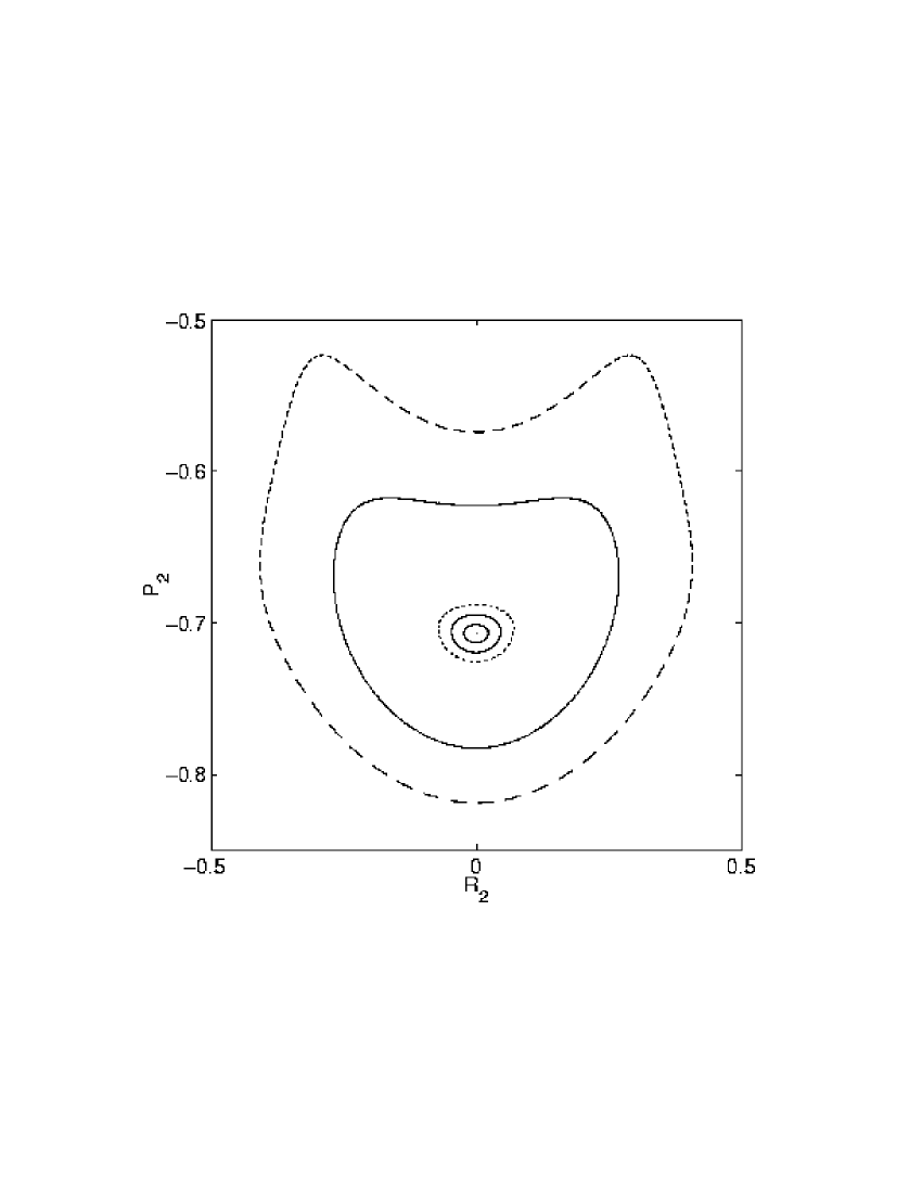
Figure 3: Poincaré sections of the four vortex system in quasiperiodic regimes. The different initial conditions correspond to continuous deformation from the square. We notice the absence of chaos resulting in closed curves. The sections are computed using the variables of the reduced system (8). The conditions imposed are the following: $R_{1}=0$, $\dot{R}_{1}<0$.

The use of these sections cannot be more conclusive, and may be at this point only a good indicator of some possible behavior of the vortex system. Indeed, a simple glance at Eq. (8) shows that the conditions $R_{1}=0$ or $R_{2}=0$ are degenerate in $\phi_{1}$ respectively $\phi_{2}$. This implies that the plotted sections are in fact a super-imposition of different sheets, which may be at the origin of the different domains observed in Fig. 2 and could also explain the difference in the center part of the plots between the chaotic sections presented in PullSaff91 and ArefPomp82 . To resolve the matter, a more detailed analysis is required, namely the order of the degeneracy has to be established, as well as its effect on the couples ($R_{1},P_{1}$), ($R_{2},P_{2}$). But even though interesting, this is beyond the scope of this paper. The sections have clearly established the desired chaotic nature of the vortex motion for our choice of initial condition. Indeed, for comparison to the chaotic case, we computed in figures 3 sections for different configurations corresponding to quasiperiodic trajectories: the difference in the nature of the trajectories is clear.

2.4 Vortex pairing

As mentioned, we use the initial condition corresponding to the chaotic trajectories of the vortices (Fig. 1). The Poincaré section illustrated in Fig. 2 suggests that the motion even though chaotic may exhibit some intermittency and for a given length of time its behavior is similar to an integrable system. As mentioned earlier on, quasi-periodic motion of four vortices can be observed for special initials conditionsArefPomp82 . Essentially the initial conditions have to be symmetrical, and since all vortices are identical the symmetry is preserved by the dynamics. This results in the loss of degrees of freedom, and allows thus for an integrable motion of the vortices. We may say that while the vortex system sticks to some domain of the phase space, it stops exploring the whole accessible phase space but remains on (sticks to) an object of lesser dimension than the total amount of degrees of freedom. In this light, stickiness can then occur when two vortex are pairing. Namely during the chaotic motion of the vortices, two vortices come close together and form a pair. The pair is for a while acting like a two-vortex system perturbed by the flow created by the two other vortices. While the pair is formed the two vortices are bound, the systems looses one degree of freedom, and as a consequence is sticking to some subdomain of the phase space. We may assume that this scenario is more likely to appear than sticking to a symmetric configuration as in the latter, the system needs to “loose” more degrees of freedom.

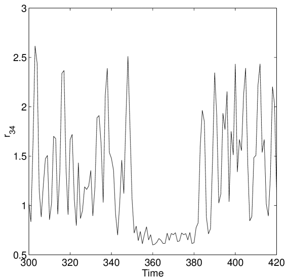
Figure 4: Typical behavior of distance between vortices versus time. The distance $r_{34}$ is plotted. A pairing of the two vortices is identified for $350<t<385$. We notice that while the pair is formed the two vortices remain close to each other ($r_{34}<1$), and the fluctuations are greatly reduced. This allows a simple diagnostic to numerically detect vortex-pairing

To detect if vortex-pairing occurs, the inter-vortex distance is measured while the evolution of the vortex is computed. The results are represented on Fig. 4 for a particular time frame, and as anticipated the pairing of vortices is observed. For the illustrated time frame, two vortices are coming close to each other around $t=350$, and remain at a distance $d\approx 0.7$ from each other for a time $\delta t\approx 30$. We notice that while the pairing occurs the inter-vortex distance remains small, and fluctuations are greatly reduced. These features allows us to detect vortex-pairings in an easy way. In regards to the previously computed Poincaré sections, it is important to mention that while a pairing occurs the two vortices are rotating at a fast pace around each other. This fast rotation is then likely to lead to “quasi-permutations” of the vortex system, and is probably the reason why we observe stickiness in Fig. 2; since none is observed in Fig. 1, we confirm that stickiness to quasi-periodic motion resulting from symmetrical initial conditions is less likely to happen than vortex-pairing.

2.5 Statistics of the pairing time

In previous work KZ2000 ; LKZpreprint , it has been clearly shown that stickiness by providing long coherent motion leads to anomalous transport properties, and distributions with power law tails. As pairing can be considered a sticky phenomenon and is very likely to influence the motion of passive tracers, it is important to obtain some statistical data on pairing times. For this purpose, a computation of vortex motion up to time $t=10^{5}$ was made. The detection of pairing events is obtained using Fig. 4: a pairing occurs if for a given length of time two vortices stay close together. This definition is rather vague and some arbitrary cutoff must be done. The arbitrary time length chosen was $\delta t=4$, which does not affect the behavior of large pairing time, and the distance from one vortex to another is such that $r_{ij}=|z_{i}-z_{j}|\leq d$. To measure the influence of this last cutoff, we chose to use three different values $d=1$, $d=0.9$ and $d=0.8$. We found enough pairings to obtain a distribution of pairings that last longer than a time $\tau$, meaning we computed the density

$$N(T>\tau)\sim\int^{\infty}_{\tau}\rho(T)dT\>,$$ (9)

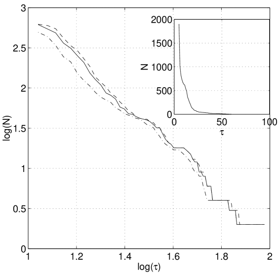
Figure 5: Number of pairings $N$ versus time length $\tau$. Only pairings lasting longer than $\tau=11$ are considered. The purpose of the different curves is to show the error-bar effects induced by the chosen inter-vortex distance cutoffs $d=0.8,\>0.9,\>1$ which respectively correspond to the dashed-dotted, solid and dashed lines. The tail of the curve shows a power law decay with coefficient $(\alpha-1)\approx-2.66$. The initial part of the curve arises error-bars. The run-time is $t=10^{5}$.

where $\rho(T)dT$ is the probability of an event to last a time $T$. The results are shown in Fig. 5, where we notice that some rare events are lasting a relatively long time, and the different curves are corresponding to different possible cutoff distance for $d$, regarding the detection of events. The analysis of the distribution’s tail is done by the Log-Log plot in Fig. 5. A power-law decay of the tail of the type $\tau^{-\alpha+1}$ with exponent $\alpha\sim 3.66\pm 0.1$ is observed, which translates in non-zero probability of very long rare events: long lasting pairing occurs. The behavior of the probability density of pairing $\rho(\tau)$ lasting a time $\tau$, is obtained from Eq. (9)

$$\rho(\tau)=\frac{dN}{d\tau}\>,$$ (10)

which leads to a power law decay of the type $\rho\sim\tau^{-\alpha}\sim\tau^{-3.7\pm 0.1}$. This behavior translates in finite average pairing time, and second moment. However since $\alpha$ is close to $4$ and the accuracy obtained for $\alpha$ is not perfect, we cannot be conclusive about the divergence of the third moment. We insist that as expected, the long-lasting time-correlations induced by a typical sticking behavior, results in a power-law decay of the distribution’s tail. We call $\alpha$ the pairing exponent and provide its estimate in the following subsection

2.6 Pairing exponent

The main idea used to obtain an estimate of the value of the paring exponent $\alpha$ follows the work presented in Ref.Zaslavsky2000 and LKZpreprint . The starting point is the occurrence of an island of stability resulting in ballistic and accelerator modes. Such islands appear in the stochastic sea as a result of a parabolic bifurcation Melnikov96 and correspond to the so-called tangled islands romkedar99 . This is a fairly general statement and it is hence reasonable to assume that the phenomenon of vortex-pairing results from the rise of such islands in the stochastic sea, i.e the formation of virtual potential well for the rotational dynamics of a pair of vortices. In this situation, we use the general form proposed in Melnikov96 and write an effective Hamiltonian for the pair of vortices (see also Zaslavsky2000 and ZEN97 ):

$$H_{eff}=c(\Delta P)^{2}-a\Delta Q_{1}-b\Delta Q_{2}-V_{3}(\Delta Q_{1},\Delta Q_{2})\>,$$ (11)

where $\Delta P$ is a generalized momentum (angular momentum) of the pair and $\Delta Q_{1},\Delta Q_{2}$ are the generalized coordinates of the corresponding vortices. The interaction potential $V_{3}$ is a third order polynomial, as higher order terms in $\Delta Q_{j}$ can be neglected for the effective Hamiltonian []; and $a$, $b$, $c$ are constants. Let us explain the expression (11) in more details.

Let us assume that the bifurcation corresponds to the appearance of an island in the stochastic see at some phase space point $\xi^{*}=(P^{*}_{1},P^{*}_{2},Q^{*}_{1},Q^{*}_{2})$. After the bifurcation occurs, the island has a finite size and any trajectory located within the island corresponds to periodic or quasiperiodic dynamics characterized by its coordinates $\xi=(P_{1},P_{2},Q_{1},Q_{2})$. It is then convenient to introduce the relative coordinates $(\Delta P_{1},\Delta P_{2},\Delta Q_{1},\Delta Q_{2})$ by $\Delta\xi=\xi-\xi^{*}$. Since the pair is rotating within a plane, in the whole phase space, we can consider that angular momentum is conserved, hence we only have one generalized momentum in Eq. (11), while the linear and cubic terms are prescribed by the nature of the bifurcation.

The following steps are fairly formal (see also ZEN97 and LKZpreprint ). Let us consider a trajectory which is close to the island’s edge. A small perturbation is then likely to allow the trajectory to “escape” from the island or its vicinity and consequently to detroy the vortex pair. The phase volume of the escaping trajectory writes:

$$\delta\Gamma=\delta P\delta Q_{1}\delta Q_{2}\>,$$ (12)

where $\delta P$ , $\delta Q_{1}$, and $\delta Q_{2}$ are the values $\Delta P$, $\Delta Q_{1}$ and $\Delta Q_{2}$ of the escaping trajectory. Since the trajectory is close to the islands edge, we can estimate from Eq.(11)

$$\delta P_{max}\sim\delta Q^{\frac{3}{2}}_{j},$$ (13)

where we have assumed $V_{3}\sim Q^{3}_{j}$, $(j=1,2)$. Using this last expression (13), we obtain for (12)

$$\delta\Gamma=\delta Q^{\frac{3}{2}}_{j}\delta Q_{1}\delta Q_{2}\sim\delta Q^{\frac{7}{2}}\>,$$ (14)

where we assumed $\delta Q_{1}\sim\delta Q_{2}\sim\delta Q$. Due to the periodic or quasiperiodic nature of the trajectories within the island, any trajectory within its neighbourhoud will have a ballistic type behavior, hence $\delta Q\sim t$, i.e

$$\delta\Gamma\sim t^{\frac{7}{2}}\>.$$ (15)

The probability density to escape the island vicinity after beeing in its neighbourhoud for a time $t$ (i.e time-length of the pairing) within an interval $dt$ is

$$\rho(t)\propto\frac{1}{\delta\Gamma(t)}\sim t^{-\frac{7}{2}}\>,$$ (16)

this results gives us directly the estimate of the exponent $\alpha\approx 7/2$, which is very close to the observed value $3.7\pm 0.1$.

Although this estimate is not rigorous, it can provide an insight on the origin of different characteristic exponents of trapping time distributions.

2.7 Minimum distance between two vortices

To conclude on vortex motion, we measure the minimum distance between two vortices. Indeed, as suggested in Babiano94 , the size of the cores surrounding the vortices is related to the minimum distance of approach between two vortices for a 3-vortex system LKZpreprint . The minimum distance is numerically measured and results are reported in Table 2, which give the value $d_{min}\approx 0.6$. An analytical estimation of the minimum inter-vortex distance can be obtained (lower bound), by assuming that the minimum occurs during a pairing, and that this minimum is small compared to the other inter-vortex distances which we can assume to be all similar to a given distance $d_{av}$. Under these conditions the the constants of motions become

$$K\equiv\left(\sum_{l=1}^{4}k_{l}\right)L^{2}-(Q^{2}+P^{2})=\sum_{l\neq m}^{4}k_{l}k_{m}|z_{i}-z_{j}|^{2}=d^{2}_{min}+5d^{2}_{av}\approx 5d^{2}_{av}\>,$$ (17)

and

$$\Lambda=\exp(-4\pi H)\approx d^{2}_{min}d^{10}_{av}\>.$$ (18)

Using both equations (17) and (18) we obtain a simple estimation for the minimum inter-vortex distance

$$d_{min}=\sqrt{\left(\frac{5}{K}\right)^{5}\Lambda}\>.$$ (19)

We now use the expression (19), with the values for the constant of motions given by the initial positions of the vortices used for the simulations: $[(1.747,1.203)$ $(-\sqrt{2}/2,0)$ $(\sqrt{2}/2,0)$ $(0,-1)]$. This leads to $d_{min}\approx 0.58$, in very good agreement with the results reported in Table 2.

Having a rough picture of the underlying vortex-motion, we now focus on the behavior of tracers.

Time of simulation	Minimum distance
$10000$	$0.6000$
$20000$	$0.5980$
$30000$	$0.5980$
$50000$	$0.5960$
$100000$	$0.5960$

Table 2: Measured minimum distance between two vortices, with respect to simulation time. We get roughly $\min(r_{ij})\sim 0.6$, which translates that the core’s radius $r$ is such that $r<0.3$.

3 Particle motion

3.1 Definitions

The evolution of a tracer is given by the advection equation

$$\dot{z}=v(z,t)$$ (20)

where $z(t)$ represent the position of the tracer at time $t$, and $v(z,t)$ is the velocity field. For a point vortex system, the velocity field is given by Eq. (3), and equation (20) can be rewritten in a Hamiltonian form:

$$\dot{z}=-2i\frac{\partial\Psi}{\partial\bar{z}},\hskip 34.14322pt\dot{\bar{z}}=2i\frac{\partial\Psi}{\partial z}$$ (21)

where the stream function

$$\Psi(z,\bar{z},t)=-\frac{1}{2\pi}\sum_{\alpha=1}^{4}k_{\alpha}\ln|z-z_{\alpha}(t)|$$ (22)

acts as a Hamiltonian. The stream function depends on time through the vortex coordinates $z_{\alpha}(t)$, implying a non-autonomous system.

3.2 Accessible phase space

A first step in understanding the motion of passive tracers is to determine their accessible domain in other words, where they move. Since the motion of the vortices which are driving the flow is chaotic, we cannot use Poincaré maps to visualize the phase space as in periodic 3-vortex systems. The possible use of Poincaré recurrences as an analog to the period should also reveal itself hazardous and numerically costly, as pairing was observed in the vortex system, and stickiness is known to alter Poincaré recurrences statistics KZ2000 ; LKZpreprint . An alternative to phase space visualization was presented in Boatto99 , where the space of initial conditions was investigated by measuring for each point its corresponding finite time Lyapunov exponent. This method was very successful and allowed to visualize “regular” regions around vortices and in the region far from the vortices, a very similar picture as the one observed in three vortex systems.

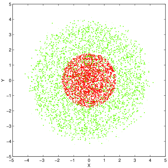
Figure 6: Accessible phase space for the particles (gray), and the four vortices (dark). The trajectories of the vortices and tracers are plotted on the plane. We notice that the tracers have access to a broader domain in agreement with results found in Boatto99 . The initial position of the tracers are taken in the region of “strong” chaos.

To confirm these results and get an idea of the accessible phase space; the positions of vortices and tracers at different times are recorded and plot in Fig. 6. This gives some first insights on the dynamics. The motion of the vortices is confined within a circular region (“ the region of strong chaos” Boatto99 ). In fact, the conservation of the angular momentum $L^{2}$ (see Eq. (5)) limits the vortex motion on a hypersphere as all vortices are identical (infinite range of motion can only be obtained with circulations of different signs). On the other hand the motion of passive tracers evolves on a much wider range. This was previously observed in Ref. Boatto99 , where it was shown that far from the region where vortices are confined, tracers diffuse radially with a vanishing diffusion rate. Contrary to three vortex systems, the chaotic nature of the vortex motions destroys the barrier observed in quasiperiodic flows which limits the chaotic sea to a finite region, and a diffusive regimes sets in.

We would like to emphasize that our choice of four identical vortices has been based first on simplicity but also on the fact that the motion of the vortices is then confined within a specific region of the plane centered around the center of vorticity. If for instance we had changed the strength of one vortex to its opposite value, sooner or later we would have observed the formation of a traveling dipole Meleshko92 . Since we consider a flow on the entire plane, the dipole will just travel towards infinity leaving behind a trivial system of two vortices. The transport properties of such systems are then dramatically modified, as the system becomes integrable as the dipole goes away, and just transient chaos is expected.

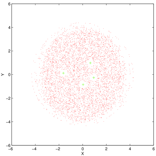
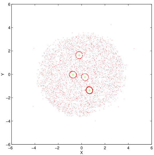
Figure 7: Snapshots of a system with 5000 particles at two different times. The vortex cores are showing, as expected. The core size is estimated around 0.3. On the bottom plot, some tracers are sticking to the cores. We also notice the almost regular motion described in Boatto99 for the far region. The initial position of the tracers are taken in the stochastic sea.

Further analysis of tracers motion is made using snapshots of the system at different times, which was used in Babiano94 to visualize the cores surrounding vortices. For this purpose $5000$ passive tracers are initially placed in the “strong chaotic region” where vortices evolve, and according to Table 2, at a distance larger than $0.3$ from any vortex. Results are presented in Fig. 7. As mentioned earlier on for the case of quasi periodic flow with four vortices Boatto99 or three KZ98 ; LKZpreprint , circular-shaped islands of regular motion are surrounding each vortex. This feature is preserved in the considered chaotic flow. Although the motion of tracers within the core is probably not regular, a barrier exists and prevents tracers to enter a a circular region around the vortex (see Fig. 7), which we will refer to as vortex “core” from now on, regular motion or not. The presence of cores in this system allows to define de facto a Lagrangian size of a point vortex. It would be therefore interesting to check if the Lagrangian definition of coherent structures boundary given in Ref. Haller2000 gives the same results: namely are the cores detected, and if so what is there size?

One snapshot illustrated Fig. 7 shows also that at certain times tracers can accumulate at the core’s boundary. This property of the tracer’s motion is crucial and was not directly addressed in previous work. In fact, this observation is very similar to the phenomenon of stickiness around vortex cores observed in 3-vortex systems, and if the analogy retains, this form stickiness should have a large influence on the transport properties of the flow, if not essential when one focuses in the area of “strong chaos” KZ2000 ; LKZpreprint .

3.3 Stickiness around the vortex core

The previous observation of both the existence of cores and the possible accumulation of tracers around cores lead to further investigations of the cores surroundings. First of all, one can wonder if the tracers can cross the barrier (if cores are analogous to porous media), which could explain the observed accumulation. Second, whether or not the barrier is crossed, it is important to know if a typical (trapping) sticking time can be defined.

A prerequisite to these questions is the estimation of the size of the core. For this matter, we placed tracers at a given distance in the vicinity of one vortex, computed its trajectory up to an arbitrary large time, and checked whether or not the tracers remained in the vicinity of the chosen vortex. A simulation was carried out for $t=5.10^{4}$. One tracer placed at a distance $r=0.25$ escapes around $t\approx 3.10^{4}$, while it remains trapped for $r=0.24$. Tracers, which are placed closer to the vortex than $r=0.24$, remain all trapped, while tracers placed at a larger distance than $r=0.25$ escape at smaller and smaller times. Therefore, given the considered initial conditions and the time spans, we estimate the size of the cores $r_{c}$ around $0.24$. And, as in the case of a three vortex system LKZpreprint , we notice that the measured value is is in good agreement with the expected upper limit of $r_{c}$ given by half the minimum inter-vortex distance (see Table 2). Moreover the fact that, as the distance from tracer to the vortex is increased, the time of escape diminishes, seems a good indicator of a stickiness phenomenon. However, the nature of the trapped tracer trajectory is unclear. A super-imposition of the two trajectories computed for $r=0.25$ and $r=0.24$ reveals a cross-over between the explored phase space, and therefore vanishing diffusion-like processes with respect to $r$ may be present. Namely, in the far region vanishing-diffusion takes place. From a tracers point of view, the region were vortices are confined becomes point like, and the flow resemble the one created by one point vortex. Symmetrically, since inter-vortex distance are bound, as the tracer is placed deeper inside the core, the flows becomes more one-point vortex like; the difference with the far region being that the core has a chaotic motion.

Once the size of the core was determined, we tried to measure the escape time $T$ of a tracer as a function of the distance from the vortex $r$, expecting from the profile of $T(r)$ to obtain a more accurate value of $r_{c}$ and information on sticking times. This attempt was unfruitful, as the dependence of the escape time $T$ on the initial position of the tracer on the circle of radius $\theta(t)$ (phase) $r$ is very sensitive. Another way to infer these properties was made by initializing a large number of tracers uniformly distributed on a circle of radius $r=0.24+\epsilon$ around one vortex, and obtain a distribution of escape times $\rho_{e}(T,r)$. This approach revealed itself also not convincing. Indeed, groups of particles are escaping a given specific times, and the frequency of these escapes is not high enough to allow us to obtain a smooth distribution $\rho_{e}(T,r)$ independent of the initial conditions of the vortex subsystem in a reasonable amount of computation time.

3.4 Tracer trapping (escaping) mechanism and core contamination

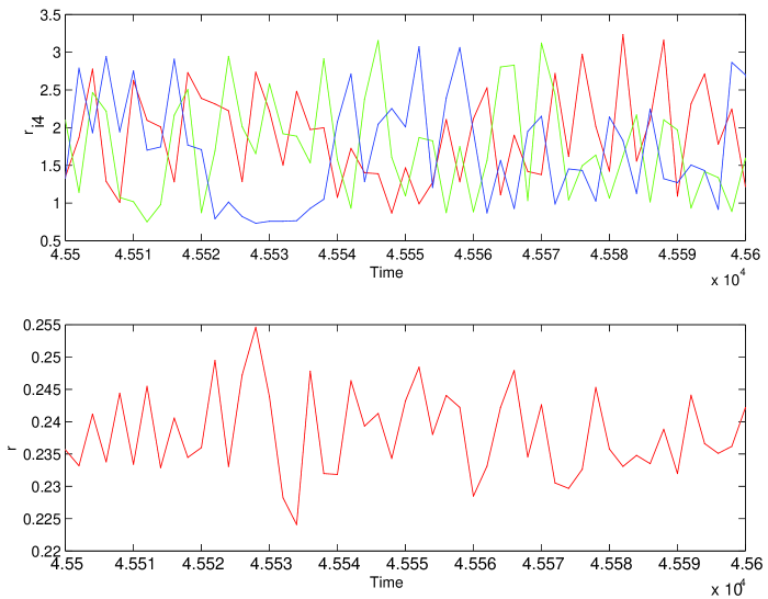
Figure 8: Distance between one vortex and the others $r_{i4}$ versus time (upper figure). We notice the pairing of two vortices around $t=4.553$ $10^{4}$. It affects the behavior of the “trapped” tracer (bottom figure). The bottom figure shows the distance $r$ between one vortex and a passive tracer ’trapped’ in the core versus time, while the pairing occurs, fluctuations are amplified. Initial vortex positions is $[(1.747,1.203)$ $(-\sqrt{2}/2,0)$ $(\sqrt{2}/2,0)$ $(0,-1)]$. Initial position of the tracer is $(0,-1.24)$ (close to the fourth vortex).

The observed sensitivity of escape times $T$ on the phase of the tracer and the strong discontinuity in $T$ of preliminary measures of $\rho_{e}(T,r)$ suggests a non uniform behavior of the vortex system, with important consequences on the vortex core surroundings. One potential candidate of this special behavior is the pairing of two vortices observed earlier on, as the relative position of the tracer to the second vortex and the sticky nature of vortex-pairing provide a good origin to the difficulties arising in the previous attempts. In a first step to check for this possible influence, a tracer was placed within the core. Its relative distance from the attached vortex is measured concurrently with the inter-vortex distances. The numerical data is collected in a time range where a pairing occurs, and the tracer is trapped in one of the vortex forming the pair. The time evolutions of the distances are presented in Fig. 8. This preliminary testings confirms that vortex-pairing has strong effects on tracers motion, as while the pairing lasts, Fig. 8 shows that fluctuations of the relative distance $r(t)$ are increased. We notice also that the increase of fluctuations goes without a noticeable jump of the averaged distance from the vortex, which points to a strong dependence on the phase of $r(t)$ during a pairing.

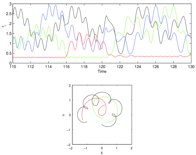
Figure 9: The upper plot shows the distances $r_{i}$ between one advected particle and the four vortices. The tracer is initially placed close to one vortex and sticks around the vortex for a certain time , then it jumps and sticks onto another vortex . After a transition time it gets back on the first vortex, we notice that the tracers has jumped to another orbit further from the vortex. At the end of the plots the particle finally escapes from the cores region. The bottom plot shows the trajectories in real space for $\delta t=4$ of time-interval ( from $t=114$ to $118$ ). The black line refers to the trajectory of the particle, while the dark and light gray lines to two the vortices involved in the jump. We note that while the jump occurs there is a “singularity” on the trajectory of the advected particle. Initial vortex position is $[(1.747,1.203)$ $(-\sqrt{2}/2,0)$ $(\sqrt{2}/2,0)$ $(0,-1)]$. The initial position of the tracer is $(0,-1.27)$.

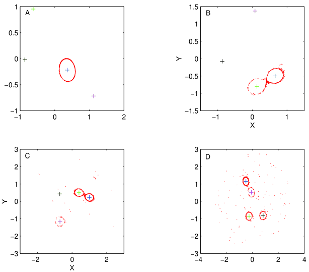
Figure 10: Four consecutive snapshots for the four vortex of equal strengths and 1000 particles, corresponding to four consecutive pairing of the vortices. Even though the particles are initially placed around one vortex, as pairings occur, some of them jump from a vortex core to another and remain on them after the pairing. While the vortex-pairing occurs some particles eventually escape from the cores. We notice also that after four pairings all cores have been “contaminated” and are populated with tracers originating from the first core and while about 10% of tracers have escaped from the region surrounding all four cores. Initial vortex position is $[(1.747,1.203)$ $(-\sqrt{2}/2,0)$ $(\sqrt{2}/2,0)$ $(0,-1)]$. Particles are uniformly initialized on the circle of radius $r=0.27$ around the fourth vortex.

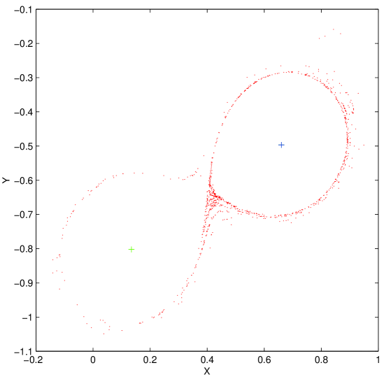
Figure 11: Zoom of Fig. 10 for the two vortex involved in the first pairing (1000 particles). The vortex on the right is the closest to the initial position of the particles. This kind of behavior is characteristic of pairing of two vortices. During the pairing of the two vortices, the periphery of the cores “merge” and form a larger “island” where particles are trapped on and may transfer from a vortex to another. Some particles may eventually escape in the process. Initial vortex position is $[(1.747,1.203)$ $(-\sqrt{2}/2,0)$ $(\sqrt{2}/2,0)$ $(0,-1)]$. Particles are uniformly initialized on the circle of radius $r=0.27$ around the fourth vortex.

Continuing our step by step investigations, we initialized $1000$ tracers on a given circle of radius $r=0.24+\epsilon$ around one vortex and made four different snapshots of the system, the first one before any pairing occurred, and the last three in the middle of 3 consecutive pairings. The results are shown on Fig. 10. This plot explain directly the observed discontinuity $\rho_{e}(T,r)$. We see that as pairing occurs the periphery of the two cores merge, allowing tracers to jump from one core to the other. In this process some tracers escape (and reversibly get trapped). When the pair is broken, each cores keeps its share of exchanged tracers and only very few tracers escape from the reformed cores. We also notice in Fig. 10 that tracers initially trapped on one core “contaminate” rapidly the other cores, and we will refer to this phenomenon as “core-contamination”. To better understand this core-contamination process a zoom of the first exchange is presented in Fig. 11. While the two vortices are bound, the local topology changes, and a peripheral merging of the cores occurs, allowing particle exchange between cores. In this quasi 2-vortex system a quasi hyperbolic point in the middle between the two vortices emerge, where the velocity field results from the contribution of the two far vortices. As a result while the tracer finds itself in this area, its motion is governed by the position of the two distant vortices, allowing it to jump from one orbit to another and possibly one core to another. A typical relative trajectory of a bound tracer is represented in Fig. 9. One notices that while the jump occurs the trajectory is singular.

These different events show the difficulty in defining properly a typical sticking time from a distribution $\rho(t,r)$, independent from the system’s initial conditions. First of all, while a tracer jumps from one core to another it continues to stick, so the sticking area has to be considered globally on the four cores, second even if particle do no jump from one core to the other, pairing allows them to jump from one orbit to another, so the dependence on $r$ of $\rho$ is unclear. Finally, as the distribution of pairing times decays as a power-law, rare events with long lasting pairings are not unprobable, implying a strong lasting dependence on initial conditions for the computation of $\rho(t,r)$. For instance in Fig. 9, after the last jump, the tracer finds itself further from the center of the core, we also notice 3 aborted jumps at $t\approx 122,\>123,\>127$, and finally around $t=130$, the tracer escapes as a last vortex approaches. Consequently, trapped particles are subject to escape from the cores as more pairing occurs, this illustrated in Fig. 10, where more and more tracers have escaped after each pairing.

We may speculate that this core-contamination phenomenon allows an unexpected type of transport for the tracers in many vortex systems. Indeed, tracers which find themselves in this peripheral zone, can jump from vortex to vortex, therefore their transport properties should match the transport properties of the sub-vortex system. Note also, that if all tracers are initially on one core like in Fig. 10 in a many vortex system the dispersion of tracers should occur mainly on the different cores, implying non typical mixing properties “targeted” to the specific region of the phase space consisting of the reunion of the periphery of all cores. This phenomenon, if persistent for more realistic systems may have some interesting practical applications. Finally, we mention that the sensitivity in these jumps from core to core in the relative position on the core of the tracer $\theta(t)$, must affect the computation of finite time Lyapunov exponents in these regions, as their value will be influenced by the chaoticity of $\theta(t)$. It is therefore possible that non-zero Lyapunov exponents are associated with trapped tracers, and we may expect a typical value related to typical pairing frequency and pairing lifetime.

3.5 Motion within the core

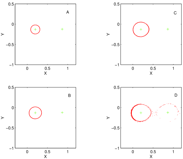
Figure 12: Different snapshots with 1000 particles, initialized at different values of the radius. The snapshots are taken while the first pairing occurs. An egg-shape form of the cluster formed by the particles appears in plot C. Suggesting a strong influence of pairing for $r>0.2$. Initial vortex position is $[(1.747,1.203)$ $(-\sqrt{2}/2,0)$ $(\sqrt{2}/2,0)$ $(0,-1)]$. Radii for the A,B,C,D plots are respectively $r=0.135$, $r=0.18$, $r=0.225$, $r=0.27$.

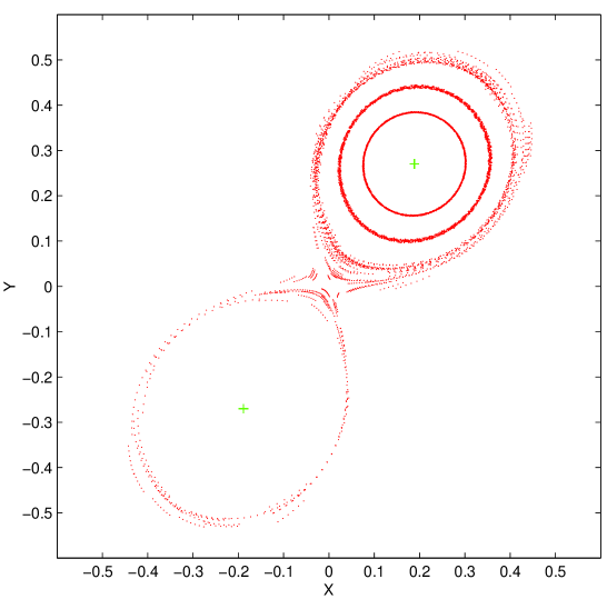
Figure 13: Trajectories of 25 advected particles, for different initial conditions The plot is made in the co-rotating frame with two vortices during a pairing lasting $\Delta t=15$, and particle positions recorded for constant inter-vortex distance. Initial vortex position is $[(1.747,1.203)$ $(-\sqrt{2}/2,0)$ $(\sqrt{2}/2,0)$ $(0,-1)]$. Particles a uniformly distributed on circles of radii: $r=0.27$, $r=.20$, $r=0.135$.

We conclude the section by briefly investigating the motion of tracers within the core. First the region within the core which is subject to a strong apparent influence from pairing is localized. For this purpose, tracers are initialized within the cores at different distances form the vortex, and a snapshot of the system is made when two vortices are pairing in Fig. 12. As expected, trajectories look more and more circular as tracers are closer to the vortex, and egg-shape deformation due to pairing appears for $r>0.2$. To confirm this statement in Fig. 13 we plotted successive positions of tracers during a pairing. The plot is made in a reference frame where the two vortices do not rotate and centered on the local center of vorticity, the position of the tracer is recorded for each time $t_{i}$ such that the distance between the two vortices $r_{12}(t_{i})$ is constant. This plot is in spirit very similar to the Poincaré maps computed in KZ98 , and gives a good insight on the local topology. However as pairing time is finite, we typically obtain only $\sim 10$ iterations of the map, which limits the resolution in Fig. 13.

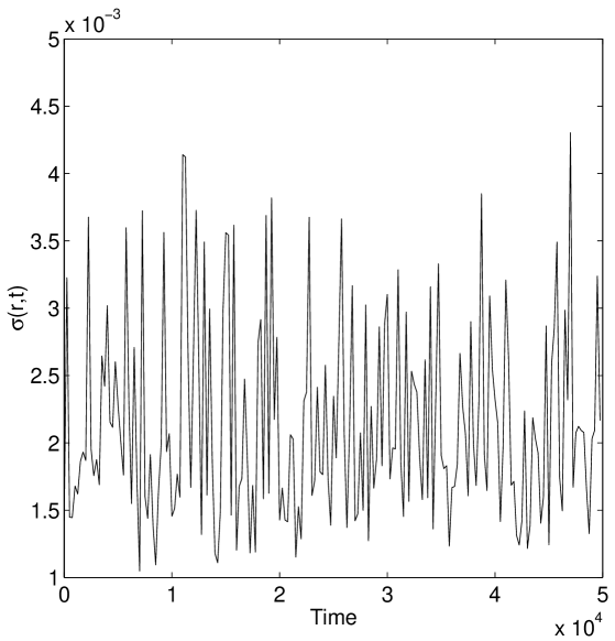
Figure 14: On the left the mean value $\langle r(t)\rangle$ as function of time is plotted. The average $\langle r(t)\rangle$ can be considered constant in time. And on the right, the standard deviation $\sigma(r,t)=\sqrt{\langle(r(t)-\langle r(t)\rangle)^{2}\rangle}$ as a function of time is plotted. We do not observe any quantitative diffusion phenomenon, and conclude on the absence of diffusion for larger times span. Data is computed using $200$ tracers. All tracers are uniformly distributed at $t=0$ on the circle of radius $r=0.18$.

Possible diffusion-like behavior of tracers need therefore be investigated deep within the core. To detect this behavior, we initialized 200 tracers on a radius $r=0.18$, and let the system evolve up to $t=5.10^{4}$. The mean and standard deviation $\langle r(t)\rangle$ and $\sigma(r,t)$ are presented in Fig. 14. We notice that for the amount of particles considered and the time-length of the simulation, no diffusive behavior is observed. All particle remain trapped on the $r=0.18$ orbit. The absence of diffusion is although not granted, but to be more conclusive we would need a larger amount of tracers, and larger times. We are then confronted with numerical problems. The divergence of the absolute speed as the vortex is approached, necessitate increasingly smaller time steps, which lead to increasingly large effective simulation times, and becomes an hindrance when one wants to compute statistics over a large number of tracers whose trajectories are computed over large times. Anyway for the time considered, the non observation of diffusion suggests that the inside of the cores are regions of almost regular motion, if not regular, and therefore cores are good trapping regions, which exchange little (if not nothing) with the outside strong chaotic region.

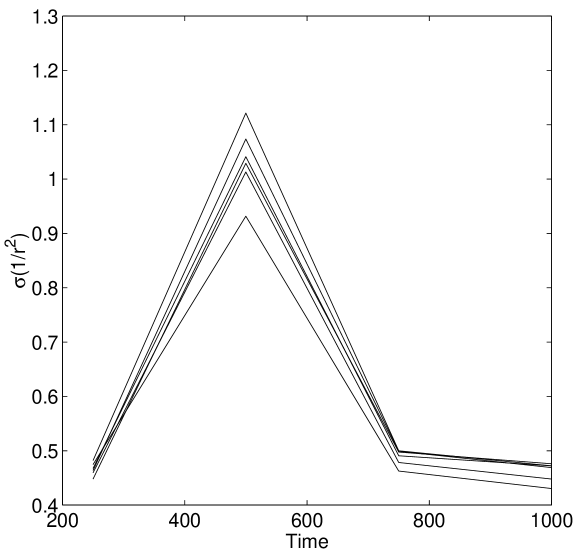
Figure 15: On the upper plot the standard deviation $\sigma(r)=\sqrt{\langle(r-\langle r\rangle)^{2}\rangle}$ as a function of the distance from the center of the vortex $r$ is represented. The log-log plot suggests a behavior $\sigma\sim r^{2.93}\sim r^{3}$. On the bottom plot the standard deviation $\sigma(1/r^{2},t)$ is computed as a function of time for the different radii used in the upper plot. All curves appear more or less to merge suggesting that $\sigma(1/r^{2},t)$ is only a function of time. Data is computed using $500$ tracers. All tracers are uniformly distributed at $t=0$ on a circle of radius $r$.

Finally the dependence of $\sigma(r,t)$ as a function of $r$ is investigated. Results show that for up to $r=0.2$, $\sigma(r)\sim r^{3}$ (see Fig. 15). This results is in fact very similar to the symmetry previously discussed between what is observed in the far region Boatto99 and the motion within the core. Namely this results translates into the fact that fluctuations scale as $\sim r^{6}$ where $r$ is the small parameter, and in the far field region it has been shown that the diffusion coefficient behaves as $D\sim 1/R^{6}$, where $R$ is the distance from the center of vorticity and $1/R$ is the small parameter. In fact we note that close to the vortex we have $\dot{\theta}\approx k/2\pi r^{2}$, therefore since $\sigma(r,t)\sim r^{3}$, we reasonably expect the standard deviation $\sigma(k/2\pi r^{2},t)\approx\sigma(\dot{\theta},t)$ to be only a function of $t$. Results are shown on Fig. 15, and we effectively notice that for all different radii, the fluctuations are more or less concentrated on one curve. It is then sufficient to consider only one orbit to study of the temporal behavior. Note also that for $r=0.18$, we obtain $\sigma(r)^{2}\sim 3.4\>10^{-5}$, so for the observed time if we had diffusion we should observe fluctuations of the order $\sigma^{2}(r,t)\sim\sigma^{2}(r)t\approx 1$ for $t=5.10^{4}$. In this light, since such growth of fluctuations was not observed in Fig.14, we can exclude the possibility of diffusive (or superdiffusive) behavior within the core. However, subdiffusive behavior is still a possibility, as for instance $(5.10^{4})^{1/8}\approx 3.87$ so the previous argument does not hold, and we need very long simulations to clarify the temporal behavior of fluctuations.

4 Conclusion

In this paper we have investigated the motion of a passive tracer in a chaotic flow generated by four identical point vortices. In the process of this study, a particular attention has been made to the vortex subsystem. Since the vortices are identical, the vortex system is subject to the additional discrete symmetry resulting from invariance through the group of permutations. This lead to introduce a new Poincaré section. This section has the advantage to exhibit the non homogeneity of the phase space, resulting from a special behavior of the vortex system corresponding to the phenomenon of vortex-pairing. Pairing results in a temporary loss of a degree of freedom of the whole systems, it is therefore associated with a stickiness phenomenon to an object of lesser dimension than the accessible phase space, and is linked to local changes of density in the Poincaré section illustrated in Fig. 2. Such behavior can then be thought of as a chaos-chaos intermittent behavior. Vortex-pairing, by involving only two vortices, is reminiscent of high-dimensional vortex systems where low-dimensional vortex behavior was shown to be influential Weiss98 . Further investigations have lead to compute pairing-time distributions. The probability density exhibits a power-law tail typical the of stickiness behavior. The power-law exponent is found to be around $\alpha\approx 3.6$, implying finite typical (average) sticking time and quantitatively agree with its analytical estimate $\alpha\approx 7/2$. We note that since most merging processes in 2D turbulence occur while two same sign-vortices are pairing, the finiteness of pairing time by the introduction of another specific time scale besides the typical merging time, may play an important role.

Passive tracers motion are analyzed for a given specific initial condition of the vortices corresponding to a chaotic flow. The emphasis is made on qualitative behavior as only one condition of the parameter space is explored and comparison is made to previous work Babiano94 ; Boatto99 as well as results obtained for quasiperiodic flows. The presence of cores surrounding the vortices is confirmed, the sticking behavior of the tracers to the cores is illustrated, and an estimation of the core size is measured, which is in good agreement with the estimation proposed in Ref. Babiano94 , given by minimum inter-vortex distance. The influence of vortex pairing on tracers dynamics is studied. This pairing phenomenon proves to be a good trapping (untrapping) mechanism explaining the observed stickiness of tracers around cores. Moreover, besides being responsible for tracers trapping, vortex-pairing allows also tracers to jump between cores. For the motion of the tracers located deep within the cores, we have shown that for the time span studied, no radial diffusion-like behavior is observed. On the other hand, the dependence of the fluctuations as a function of the distance from the vortex is measured and these are shown to scale as $r^{6}$, which gives, in regards to the small parameter, the same order as the scaling previously computed in the far field region in Ref. Boatto99 .

To conclude, the motion of a passive tracer in the chaotic flow generated by four point vortices has four different typical behaviors in four distinct regions of the phase space. In the far field region, its motion is almost regular, with some irregular jumps from one orbit to the other. Its motion is chaotic in the region of “strong chaos”, corresponding to the area where the vortex motion is restricted (see Boatto99 ). In the periphery of the cores, tracers can stick to one core and travel with one specific vortex, as well as travel through the phase space by jumping from one core to another. Finally deep inside the vortex core, the tracers remain trapped on a specific orbit for the observed time length of our simulations, and travel with the corresponding vortex. Transport properties are subject to the influence of regions to which a tracer has access, which counts all regions besides the inner of the cores. The existence of stickiness on vortex cores and regular motion in the far field region allows us, by analogy with three vortex systems KZ2000 ; LKZpreprint , to speculate that long time behavior of tracers is governed by these two regions. Each of them dominating one part of the moments, namely the low moments for the far field region, and the high moments for the periphery of cores. Moreover, the possibility for sticking tracers to jump from core to core, leads to anticipate on the existence of special transport features in many vortex systems. It is indeed likely that this feature allows to transport highly concentrated regions of passive tracers over large distances with controlled dilution and at fast pace. Namely, in many vortex systems, contrary to tracers located within one core which are transported by one and only vortex and hence may be trapped for relatively long times in some slow moving cluster of vortices. Those located on the core’s periphery should quickly spread on all other cores periphery and therefore populate the whole space accessible to the vortices; but by remaining on the cores, the spreading should occur with relatively little dilution compared to the region of strong chaos.

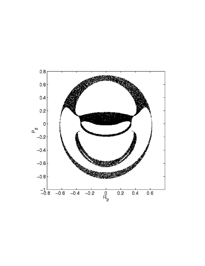
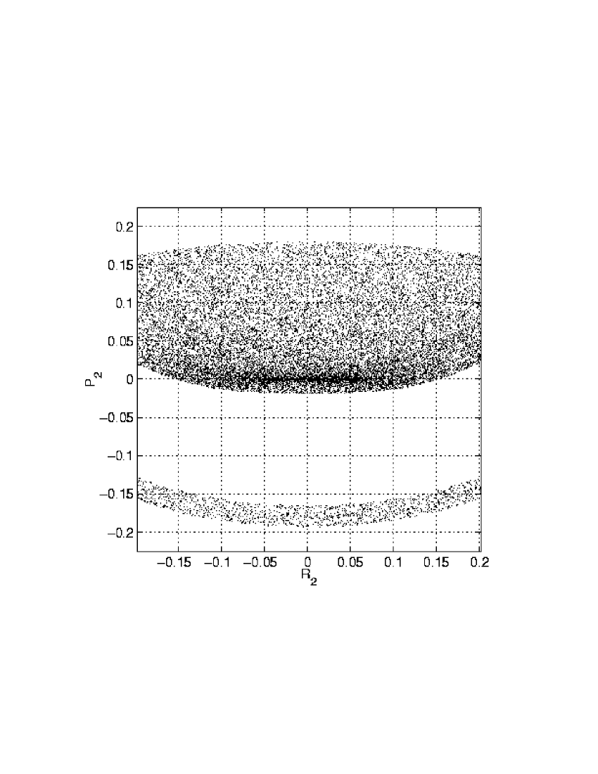
Figure 2: Poincaré section of the four vortex system in the chaotic regime for a given initial condition. The section is computed using the variables of the reduced system (8). The conditions imposed are the following: $R_{1}=0$, $\dot{R}_{1}<0$. This section has the advantage of containing all equivalent physical configurations resulting from any permutation of the vortices. Consequently stickiness is observed, while it was not in Fig. 1. The lower plot is a zoom of the upper one.

References

- (1) H.Aref, Stirring by chaotic advection, J. Fluid Mech. 143, 1 (1984)
- (2) G. M. Zaslavsky, R. Z. Sagdeev, and A. A. Chernikov, Zhurn. Eksp. Teor. Fiz. 94, 102 (1988) (Soviet Physics, JETP 67, 270 (1988)
- (3) J. Ottino, The kinematics of Mixing: Stretching, Chaos, and Transport (Cambrige U. P., Cambrige, 1989)
- (4) H.Aref, Chaotic advection of fluid particles, Phil. Trans. R. Soc. London A 333, 273 (1990)
- (5) J. Ottino, Mixing, Chaotic advection and turbulence, Ann. Rev. Fluid Mech. 22, 207 (1990)
- (6) V. Rom-Kedar, A. Leonard and S. Wiggins, An analytical study of transport mixing and chaos in an unsteady vortical flow, J. Fluid Mech. 214, 347 (1990)
- (7) G. M. Zaslavsky, R. Z. Sagdeev, D. A. Usikov, and A. A. Chernikov, Weak Chaos and Quasiregular Patterns, Cambridge Univ. Press, (Cambridge 1991)
- (8) A. Crisanti, M. Falcioni, G. Paladin and A. Vulpiani, Lagrangian Chaos: Transport, Mixing and Diffusion in Fluids, La Rivista del Nuovo Cimento, 14, 1 (1991)
- (9) A. Crisanti, M. Falcioni, A. Provenzale, P. Tanga and A. Vulpiani, Dynamics of passively advected impurities in simple two-dimensional flow models, Phys. Fluids A 4, 1805 (1992)
- (10) A. Provenzale, Transport by Coherent Barotropic Vortices, Annu. Rev. Fluid Mech. 31, 55 (1999)
- (11) A. J. Majda, J. P. Kramer, Simplified models for turbulent diffusion: Theory, numerical modeling, and physical phenomena, Phys. Rep. 314, 238 (1999)
- (12) J. B. Weiss, A. Provenzale, J. C. McWilliams, Lagrangian dynamics in high-dimensional point-vortex system, Phys. Fluids 10, 1929 (1998)
- (13) P. Tabeling, A.E. Hansen, J. Paret, Forced and Decaying 2D turbulence: Experimental Study, in “Chaos, Kinetics and Nonlinear Dynamics in Fluids and Plasma”, eds. Sadruddin Benkadda and George Zaslavsky, p. 145, (Springer 1998)
- (14) A. E Hansen, D. Marteau , P. Tabeling, Two-dimensional turbulence and dispersion in a freely decaying system, Phys. Rev. E 58, 7261 (1998)
- (15) P. Tabeling, S. Burkhart, O. Cardoso, H. Willaime, Experimental-Study of Freely Decaying 2-Dimensional Turbulence, Phys. Rev. Lett. 67, 3772 (1991)
- (16) V.V. Meleshko, M.Yu. Konstantinov, Vortex Dynamics and Chaotic Phenomena, (World Scientific, Singapore, 1999)
- (17) R. Benzi, G. Paladin, S. Patarnello, P. Santangelo and A. Vulpiani, Intermittency and coherent structures in two-dimensional turbulence, J. Phys A 19, 3771 (1986)
- (18) R. Benzi, S. Patarnello and P. Santangelo, Self-similar coherent structures in two-dimensional decaying turbulence, J. Phys A 21, 1221 (1988)
- (19) J. B. Weiss, J. C. McWilliams, Temporal scaling behavior of decaying two-dimensional turbulence, Phys. Fluids A 5, 608 (1992)
- (20) J. C. McWilliams, The emergence of isolated coherent vortices in turbulent flow, J. Fluid Mech. 146, 21 (1984)
- (21) J. C. McWilliams, The vortices of two-dimensional turbulence, J. Fluid Mech. 219, 361 (1990)
- (22) D. Elhmaïdi, A. Provenzale and A. Babiano, Elementary topology of two-dimensional turbulence from a Lagrangian viewpoint and single particle dispersion, J. Fluid Mech. 257, 533 (1993)
- (23) G. F. Carnevale, J. C. McWilliams, Y. Pomeau, J. B. Weiss and W. R. Young, Evolution of Vortex Statistics in Two-Dimensional Turbulence, Phys. Rev. Lett. 66, 2735 (1991)
- (24) N. J. Zabusky, J. C. McWilliams, A modulated point-vortex model for geostrophic, -plane dynamics, Phys. Fluids 25, 2175 (1982)
- (25) P. W. C. Vobseek, J. H. G. M. van Geffen,, V. V. Meleshko, G. J. F. van Heijst, Collapse interaction of finite-sized two-dimensional vortices, Phys. Fluids 9, 3315 (1997)
- (26) O. U. Velasco Fuentes, G. J. F. van Heijst, N. P. M. van Lipzig, Unsteady behaviour of a topography-modulated tripole, J. Fluid Mech. 307, 11 (1996)
- (27) R. Benzi, M. Colella, M. Briscolini, and P. Santangelo, A simple point vortex model for two-dimensional decaying turbulence, Phys. Fluids A 4, 1036 (1992)
- (28) J. B. Weiss, Punctuated Hamiltonian Models of Structured Turbulence, in Semi-Analytic Methods for the Navier-Stokes Equations, CRM Proc. Lecture Notes, 20, 109, (1999)
- (29) D. G. Dritschel, N. J. Zabusky, On the nature of the vortex interactions and models in unforced nearly-inviscid two-dimensional turbulence, Phys. Fluids 8(5), 1252 (1996)
- (30) A. Aref, Turbulent Statistical dynamics of a system of point vortices, in “Trends in Mathematics”, p 151 (Birkhäuser Verlag 1999)
- (31) C. Sire and P. H. Chavanis, Numerical renormalization group of the vortex aggregation in 2D decaying turbulence: the role of three-body interactions. Phys. Rev. E 61, 6644 (2000)
- (32) A. A. Chernikov, B. A. Petrovichev, A. V. Rogal’sky, R. Z. Sagdeev, and G. M. Zaslavsky, Anomalous Transport of Streamlines Due to their Chaos and their Spatial Topology, Phys. Lett. A 144, 127 (1990)
- (33) T.H. Solomon, E.R. Weeks, H.L. Swinney, Chaotic advection in a two-dimensional flow: Lévy flights in and anomalous diffusion, Physica D, 76, 70 (1994)
- (34) E.R. Weeks, J.S. Urbach, H.L. Swinney, Anomalous diffusion in asymmetric random walks with a quasi-geostrophic flow example, Physica D, 97, 219 (1996)
- (35) G.M. Zaslavsky, D. Stevens, H. Weitzner, Self-similar transport in incomplete chaos, Phys. Rev E 48, 1683 (1993)
- (36) S. Kovalyov, Phase space structure and anomalous diffusion in a rotational fluid experiment, Chaos 10, 153 (2000)
- (37) G. Haller and G. Yuan, Lagrangian coherent structures and mixing in two-dimesnional turbulence, Preprint (2000)
- (38) L. Kuznetsov and G.M. Zaslavsky, Regular and Chaotic advection in the flow field of a three-vortex system, Phys. Rev E 58, 7330 (1998).
- (39) Z. Neufeld and T. Tél, The vortex dynamics analogue of the restricted three-body problem: advection in the field of three identical point vortices, J. Phys. A: Math. Gen. 30, 2263 (1997)
- (40) L. Kuznetsov and G. M. Zaslavsky, Passive particle transport in three-vortex flow. Phys. Rev. E. 61, 3777 (2000).
- (41) X. Leoncini, L. Kuznetsov and G. M. Zaslavsky, Chaotic advection near 3-vortex Collapse, To be published in Phys. Rev. E.
- (42) H. Aref, Motion of three vortices, Phys. Fluids 22, 393 (1979)
- (43) H. Aref, Integrable, chaotic and turbulent vortex motion in two-dimensional flows, Ann. Rev. Fluid Mech. 15, 345 (1983)
- (44) E. A. Novikov, Dynamics and statistics of a system of vortices, Sov. Phys. JETP 41, 937 (1975)
- (45) J. L. Synge, On the motion of three vortices, Can. J. Math. 1, 257 (1949)
- (46) X. Leoncini, L. Kuznetsov and G. M. Zaslavsky, Motion of Three Vortices near Collapse, Phys. Fluids 12, 1911 (2000)
- (47) J. Tavantzis and L. Ting, The dynamics of three vortices revisited, Phys. Fluids 31, 1392 (1988)
- (48) E. A. Novikov, Yu. B. Sedov, Stochastic properties of a four-vortex system, Sov. Phys. JETP 48, 440 (1978)
- (49) H. Aref and N. Pomphrey, Integrable and chaotic motions of four vortices: I. the case of identical vortices, Proc. R. Soc. Lond. A 380, 359 (1982).
- (50) S. L. Ziglin, Nonintegrability of a problem on the motion of four point vortices, Sov. Math. Dokl. 21, 296 (1980)
- (51) A. Babiano, G. Boffetta, A. Provenzale and A. Vulpiani, Chaotic advection in point vortex models and two-dimensional turbulence, Phys. Fluids 6, 2465 (1994)
- (52) S. Boatto and R. T. Pierrehumbert, Dynamics of a passive tracer in a velocity field of four identical point vortices. J. Fuild Mech. 394, 137 (1999).
- (53) H. Lamb, Hydrodynamics, (6th ed. New York, Dover, 1945).
- (54) D. I. Pullin and P. G. Saffman, Long-time symplectic integration: the example of four-vortex motion, Proc. R. Soc. Lond. A 432, 481 (1991).
- (55) R.I. McLachlan, P. Atela, The accuracy of symplectic integrators, Nonlinearity 5, 541 (1992).
- (56) G. M. Zaslavsky and M. Edelman, Hierarchical structures in the phase space and fractional kinetics: I. Classical systems, Chaos 10, 135 (2000).
- (57) V. K. Melnikov, On the existence of self-similar structures in the resonnance domain, in Transport, Chaos and Plasma Physics II, Proceedings, Marseille, edited by F. Doveil, S. Benkadda, and Y. Elskens (World Scientific, Singapore, 1996), pp. 142-153
- (58) V. Rom-Kedar and G. M. Zaslavsky, Islands of accelerator modes and homoclinic tangles, Chaos 9, 697 (1999)
- (59) G. M. Zaslavsky, M. Edelman, B. A. Niyazov, Self-similarity, renormalization, and phase space nonuniformity of Hamiltonian chaotic dynamics, Chaos
- (60) V.V. Melezhko, M.Yu. Konstantinov, A.A. Gurzhi and T.P. Konovaljuk, Advection of a vortex pair atmosphere in a velocity field of point vortices, Phys. Fluids A 4, 2779 (1992)