Confidence intervals for the parameter of Poisson distribution in presence of background

I Introduction

In paper [1] the unified approach to the construction of confidence intervals and confidence limits for a signal with a background presence, in particular for Poisson distributions, has been proposed. The method is widely used for the presentation of physical results [2] though a number of investigators criticize this approach [3]

In present paper we use a simple method for construction of confidence intervals for parameter of Poisson distribution for signal in the presence of background which has Poisson distribution with known value of parameter. This method is based on the statement [4] that the true value of parameter of the Poisson distribution in the case of observed number of events $\hat{x}$ has a Gamma distribution. In contrast to the approach proposed in [1], the width of confidence intervals in the case of $\hat{x}=0$ is independent on the value of the parameter of the background distribution. The described procedure has both Bayesian and frequentist interpretations.

In Section 2 the method of construction of confidence intervals for parameter of Poisson distribution for signal in the presence of background which has Poisson distribution with known value of parameter is described. The results of confidence intervals construction and their comparison with the results of unified approach are also given in the Section 2. The main results of this note are formulated in the Conclusion.

II The method of construction of confidence intervals

Assume that in the experiment with the fixed integral luminosity (i.e. a process under study may be considered as a homogeneous process during given time) the $\hat{x}$ events of some Poisson process were observed. It means that we have an experimental estimation $\hat{\lambda}(\hat{x})$ of the parameter $\lambda$ of Poisson distribution. We have to construct a confidence interval $(\hat{\lambda}_{1}(\hat{x}),\hat{\lambda}_{2}(\hat{x}))$, covering the true value of the parameter $\lambda$ of the distribution under study with confidence level $1-\alpha$, where $\alpha$ is a significance level. It is known from the theory of statistics [5], that the mean value of a sample of data is an unbiased estimation of mean of distribution under study. In our case the sample consists of one observation $\hat{x}$. For the discrete Poisson distribution the mean coincides with the estimation of parameter value, i.e. $\hat{\lambda}=\hat{x}$ in our case. As it is shown in ref [4] the true value of parameter $\lambda$ has Gamma distribution $\Gamma_{1,\hat{x}+1}$, where the scale parameter is equal to 1 and the shape parameter is equal to $\hat{x}+1$ (see Fig.1), i.e.

$$P(\lambda|\hat{x})=P(\hat{x}|\lambda)=\displaystyle\frac{\lambda^{\hat{x}}}{\hat{x}!}e^{-\lambda}.$$ (1)

Note that formula (2.1) results from the Bayesian formula [6]

$$P(\lambda|\hat{x})P(\hat{x})=P(\hat{x}|\lambda)P(\lambda)$$ (2)

in the assumption that all possible values of parameter $\lambda$ have equal probability, i.e. $P(\lambda)=const$. In this assumption the probability that unknown parameter $\lambda$ obeys the inequalities $\lambda_{1}~{}\leq~{}\lambda~{}\leq~{}\lambda_{2}$ is given by evident Bayesian formula

$$P(\lambda_{1}\leq\lambda\leq\lambda_{2}|\hat{x})=P(\lambda_{1}\leq\lambda|\hat{x})-P(\lambda_{2}\leq\lambda|\hat{x})=\int_{\lambda_{1}}^{\lambda_{2}}{P(\lambda|\hat{x})d\lambda},$$ (3)

$P(\lambda_{1}\leq\lambda|\hat{x})=\int_{\lambda_{1}}^{\infty}{P(\lambda|\hat{x})d\lambda}$,

where $P(\lambda|\hat{x})$ is determined by formula (2.1).

Formula (2.3) has also well defined frequentist meaning. Using the identity

$$\sum_{i=\hat{x}+1}^{\infty}{\frac{\lambda_{1}^{i}e^{-\lambda_{1}}}{i!}}+\int_{\lambda_{1}}^{\lambda_{2}}{\frac{\lambda^{\hat{x}}e^{-\lambda}}{\hat{x}!}d\lambda}+\sum_{i=0}^{\hat{x}}{\frac{\lambda_{2}^{i}e^{-\lambda_{2}}}{i!}}=1$$ (4)

one can rewrite formula (2.3) as

$$P(\lambda_{1}~{}\leq~{}\lambda~{}\leq~{}\lambda_{2}|\hat{x})=1-P(n\leq\hat{x}|\lambda_{2})-P(n>\hat{x}|\lambda_{1})=P(n\leq\hat{x}|\lambda_{1})-P(n\leq\hat{x}|\lambda_{2}),$$ (5)

where $P(n\leq\hat{x}|\lambda)=\displaystyle\sum_{n=0}^{\hat{x}}{\frac{\lambda^{n}e^{-\lambda}}{n!}}$ and $P(n>\hat{x}|\lambda)=\displaystyle\sum_{n=\hat{x}+1}^{\infty}{\frac{\lambda^{n}e^{-\lambda}}{n!}}$.

The right hand side of formula (2.5) has well defined frequentist meaning and in fact it is one of the possible definitions of the confidence interval in frequentist approach . As an example, such type the shortest 90% CL confidence interval in case of observed number of events $\hat{x}=4$ is shown in Fig.2.

For instance, for the case $\lambda_{2}=\infty$ formula (2.5) takes the form

$$\int_{\lambda_{1}}^{\infty}{P(\lambda|\hat{x})d\lambda}=P(\lambda_{1}\leq\lambda|\hat{x})=\sum_{n=0}^{\hat{x}}{P(n|\lambda_{1})}=P(n\leq\hat{x}|\lambda_{1}),$$ (6)

which has evident frequentist meaning too.

Let us consider the Poisson distribution with two components: signal component with a parameter $\lambda_{s}$ and background component with a parameter $\lambda_{b}$, where $\lambda_{b}$ is known. To construct confidence intervals for parameter $\lambda_{s}$ of signal in the case of observed value $\hat{x}$ we must find the distribution $P(\lambda_{s}|\hat{x})$.

At first let us consider the simplest case $\hat{x}=\hat{s}+\hat{b}=1$. Here $\hat{s}$ is a number of signal events and $\hat{b}$ is a number of background events among observed $\hat{x}$ events.

The $\hat{b}$ can be equal to 0 and to 1. We know that the $\hat{b}$ is equal to 0 with probability

$$p_{0}=P(\hat{b}=0)=\displaystyle\frac{\lambda_{b}^{0}}{0!}e^{-\lambda_{b}}=e^{-\lambda_{b}}$$ (7)

and the $\hat{b}$ is equal to 1 with probability

$$p_{1}=P(\hat{b}=1)=\displaystyle\frac{\lambda_{b}^{1}}{1!}e^{-\lambda_{b}}=\lambda_{b}e^{-\lambda_{b}}.$$ (8)

Correspondingly, $P(\hat{b}=0|\hat{x}=1)=P(\hat{s}=1|\hat{x}=1)=\displaystyle\frac{p_{0}}{p_{0}+p_{1}}$ and $P(\hat{b}=1|\hat{x}=1)=P(\hat{s}=0|\hat{x}=1)=\displaystyle\frac{p_{1}}{p_{0}+p_{1}}$.

It means that distribution of $P(\lambda_{s}|\hat{x}=1)$ is equal to sum of distributions

$$P(\hat{s}=1|\hat{x}=1)\Gamma_{1,2}+P(\hat{s}=0|\hat{x}=1)\Gamma_{1,1}=\displaystyle\frac{p_{0}}{p_{0}+p_{1}}\Gamma_{1,2}+\displaystyle\frac{p_{1}}{p_{0}+p_{1}}\Gamma_{1,1},$$ (9)

where $\Gamma_{1,1}$ is Gamma distribution with probability density $P(\lambda_{s}|\hat{s}=0)=\displaystyle e^{-\lambda_{s}}$ and $\Gamma_{1,2}$ is Gamma distribution with probability density $P(\lambda_{s}|\hat{s}=1)=\displaystyle\lambda_{s}e^{-\lambda_{s}}$. As a result we have

$$P(\lambda_{s}|\hat{x}=1)=\displaystyle\frac{\lambda_{s}+\lambda_{b}}{1+\lambda_{b}}\displaystyle e^{-\lambda_{s}}.$$ (10)

Using formula (2.10) for $P(\lambda_{s}|\hat{x}=1)$ and formula (2.5) we construct the shortest confidence interval of any confidence level in a trivial way.

In this manner we can construct the distribution of $P(\lambda_{s}|\hat{x})$ for any values of $\hat{x}$ and $\lambda_{b}$. As a result we have obtained the known formula .

$$P(\lambda_{s}|\hat{x})=\displaystyle\frac{(\lambda_{s}+\lambda_{b})^{\hat{x}}}{\hat{x}!\displaystyle\sum_{i=0}^{\hat{x}}{\lambda_{b}^{i}\over{i!}}}\displaystyle e^{-\lambda_{s}}.$$ (11)

The numerical results for the confidence intervals and for comparison the results of paper [1] are presented in Table 1 and Table 2.

It should be noted that in our approach the dependence of the width of confidence intervals for parameter $\lambda_{s}$ on the value of $\lambda_{b}$ in the case $\hat{x}=0$ is absent. For $\hat{x}=0$ the method proposed in ref. [10] also gives a 90% upper limit independent of $\lambda_{b}$. This dependence is absent also in Bayesian approach [8, 11].

III Conclusion

The results of construction of frequentist confidence intervals for the parameter $\lambda_{s}$ of Poisson distribution for the signal in the presence of background with known value of parameter $\lambda_{b}$ are presented. It is shown that the described procedure has both Bayesian and frequentist interpretations.

Acknowledgments

We are grateful to V.A. Matveev, V.F. Obraztsov and Fred James for the interest to this work and for valuable comments. We wish to thank S.S. Bityukov, A.V. Dorokhov, V.A. Litvine and V.N. Susoikin for useful discussions. This work has been supported by RFFI grant 99-02-16956 and grant INTAS-CERN 377.

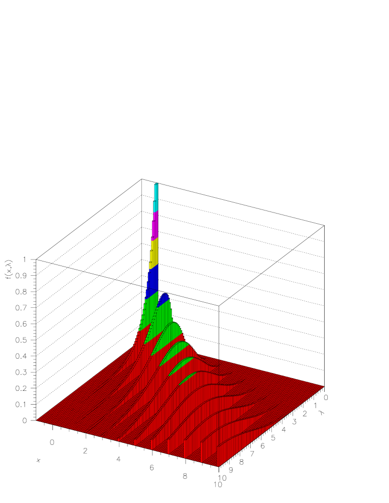
FIG. 1.: The behaviour of the probability density of true value of parameter $\lambda$ for Poisson distribution in case of $x$ observed events versus $\lambda$ and $x$. Here $f(x,\lambda)=\displaystyle\frac{\lambda^{x}}{x!}e^{-\lambda}$ is both a Poisson distribution with parameter $\lambda$ along the axis $x$ and a Gamma distribution with a shape parameter $x+1$ and a scale parameter 1 along the axis $\lambda$.

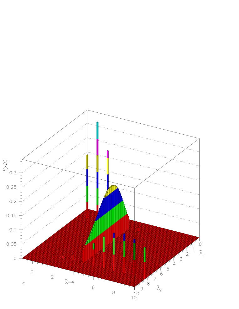
FIG. 2.: The Poisson distributions $f(x,\lambda)$ for $\lambda$’s determined by the confidence limits $\hat{\lambda}_{1}=1.51$ and $\hat{\lambda}_{2}=8.36$ in case of observed number of events $\hat{x}=4$ are shown. The probability density of Gamma distribution with scale parameter $a=1$ and shape parameter $x=\hat{x}=4$ is shown inside this confidence interval.

TABLE I.: 90% C.L. intervals for the Poisson signal mean $\lambda_{s}$, for total events observed $\hat{x}$, for known mean background $\lambda_{b}$ ranging from 0 to 4. A comparison between results of ref.[1] and results from present note.

$\hat{x}\backslash\lambda_{b}$	0.0 ref.[1]	0.0	1.0 ref.[1]	1.0	2.0 ref.[1]	2.0	3.0 ref.[1]	3.0	4.0 ref.[1]	4.0
0	0.00, 2.44	0.00, 2.30	0.00, 1.61	0.00, 2.30	0.00, 1.26	0.00, 2.30	0.00, 1.08	0.00, 2.30	0.00, 1.01	0.00, 2.30
1	0.11, 4.36	0.09, 3.93	0.00, 3.36	0.00, 3.27	0.00, 2.53	0.00, 3.00	0.00, 1.88	0.00, 2.84	0.00, 1.39	0.00, 2.74
2	0.53, 5.91	0.44, 5.48	0.00, 4.91	0.00, 4.44	0.00, 3.91	0.00, 3.88	0.00, 3.04	0.00, 3.53	0.00, 2.33	0.00, 3.29
3	1.10, 7.42	0.93, 6.94	0.10, 6.42	0.00, 5.71	0.00, 5.42	0.00, 4.93	0.00, 4.42	0.00, 4.36	0.00, 3.53	0.00, 3.97
4	1.47, 8.60	1.51, 8.36	0.74, 7.60	0.51, 7.29	0.00, 6.60	0.00, 6.09	0.00, 5.60	0.00, 5.35	0.00, 4.60	0.00, 4.78
5	1.84, 9.99	2.12, 9.71	1.25, 8.99	1.15, 8.73	0.43, 7.99	0.20, 7.47	0.00, 6.99	0.00, 6.44	0.00, 5.99	0.00, 5.72
6	2.21,11.47	2.78,11.05	1.61,10.47	1.79,10.07	1.08, 9.47	0.83, 9.01	0.15, 8.47	0.00, 7.60	0.00, 7.47	0.00, 6.76
7	3.56,12.53	3.47,12.38	2.56,11.53	2.47,11.38	1.59,10.53	1.49,10.37	0.89, 9.53	0.57, 9.20	0.00, 8.53	0.00, 7.88
8	3.96,13.99	4.16,13.65	2.96,12.99	3.18,12.68	2.14,11.99	2.20,11.69	1.51,10.99	1.21,10.60	0.66, 9.99	0.34, 9.33
9	4.36,15.30	4.91,14.95	3.36,14.30	3.91,13.96	2.53,13.30	2.90,12.94	1.88,12.30	1.92,11.94	1.33,11.30	0.97,10.81
10	5.50,16.50	5.64,16.21	4.50,15.50	4.66,15.22	3.50,14.50	3.66,14.22	2.63,13.50	2.64,13.21	1.94,12.50	1.67,12.16
20	13.55,28.52	13.50,28.33	12.55,27.52	12.53,27.34	11.55,26.52	11.53,26.34	10.55,25.52	10.53,25.34	9.55,24.52	9.53,24.34

TABLE II.: 90% C.L. intervals for the Poisson signal mean $\lambda_{s}$, for total events observed $\hat{x}$, for known mean background $\lambda_{b}$ ranging from 6 to 15. A comparison between results of ref.[1] and results from present note.

$\hat{x}\backslash\lambda_{b}$	6.0 ref.[1]	6.0	8.0 ref.[1]	8.0	10.0 ref.[1]	10.0	12.0 ref.[1]	12.0	15.0 ref.[1]	15.0
0	0.00, 0.97	0.00, 2.30	0.00, 0.94	0.00, 2.30	0.00, 0.93	0.00, 2.30	0.00, 0.92	0.00, 2.30	0.00, 0.92	0.00, 2.30
1	0.00, 1.14	0.00, 2.63	0.00, 1.07	0.00, 2.56	0.00, 1.03	0.00, 2.51	0.00, 1.00	0.00, 2.48	0.00, 0.98	0.00, 2.45
2	0.00, 1.57	0.00, 3.01	0.00, 1.27	0.00, 2.85	0.00, 1.15	0.00, 2.75	0.00, 1.09	0.00, 2.68	0.00, 1.05	0.00, 2.61
3	0.00, 2.14	0.00, 3.48	0.00, 1.49	0.00, 3.20	0.00, 1.29	0.00, 3.02	0.00, 1.21	0.00, 2.91	0.00, 1.14	0.00, 2.78
4	0.00, 2.83	0.00, 4.04	0.00, 1.98	0.00, 3.61	0.00, 1.57	0.00, 3.34	0.00, 1.37	0.00, 3.16	0.00, 1.24	0.00, 2.98
5	0.00, 4.07	0.00, 4.71	0.00, 2.60	0.00, 4.10	0.00, 1.85	0.00, 3.72	0.00, 1.58	0.00, 3.46	0.00, 1.32	0.00, 3.20
6	0.00, 5.47	0.00, 5.49	0.00, 3.73	0.00, 4.67	0.00, 2.40	0.00, 4.15	0.00, 1.86	0.00, 3.80	0.00, 1.47	0.00, 3.46
7	0.00, 6.53	0.00, 6.38	0.00, 4.58	0.00, 5.34	0.00, 3.26	0.00, 4.65	0.00, 2.23	0.00, 4.19	0.00, 1.69	0.00, 3.74
8	0.00, 7.99	0.00, 7.35	0.00, 5.99	0.00, 6.10	0.00, 4.22	0.00, 5.23	0.00, 2.83	0.00, 4.64	0.00, 1.95	0.00, 4.06
9	0.00, 9.30	0.00, 8.41	0.00, 7.30	0.00, 6.95	0.00, 5.30	0.00, 5.89	0.00, 3.93	0.00, 5.15	0.00, 2.45	0.00, 4.42
10	0.22,10.50	0.02, 9.53	0.00, 8.50	0.00, 7.88	0.00, 6.50	0.00, 6.63	0.00, 4.71	0.00, 5.73	0.00, 3.00	0.00, 4.83
20	7.55,22.52	7.53,22.34	5.55,20.52	5.53,20.34	3.55,18.52	3.55,18.30	2.23,16.52	1.70,16.08	0.00,13.52	0.00,12.31

REFERENCES

- [1] Feldman, G.J. and R.D. Cousins, Unified approach to the classical statistical analysis of small signal, Phys.Rev. D57 3873-3889 (1998).
- [2] Groom, D.E. et al., Review of particle physics, Eur.Phys.J. C 15 (2000) 198-199.
- [3] as an example, Zech, G., Classical and Bayesian Confidence Limits, in: F. James, L. Lyons, and Y. Perrin (Eds.), Proc. of 1st Workshop on Confidence Limits, CERN 2000-005, Geneva, Switzerland, (2000) 141-154.
- [4] Bityukov S.I, N.V. Krasnikov and V.A. Taperechkina, On the confidence interval for the parameter of Poisson distribution. e-print arXiv: physics/0008082, August 2000.
- [5] as an example, Handbook of Probability Theory and Mathematical Statistics (in Russian), V.S. Korolyuk (Ed.), (Kiev, ”Naukova Dumka”, 1978)
- [6] Rainwater L.J. and C.S. Wu, Nucleonics 1 (1947) 60
- [7] Cousins R.D. Why isn’t every physicist a Baysian ? Am.J.Phys 63 (1995) 398-410.
- [8] D’Agostini G., Bayesian Reasoning in High-Energy Physics: Principles and Applications. Yellow Report CERN 99-03, Geneva, Switzerland, (1999); also D’Agostini G., e-print arXiv: hep-ph/9512295, December 1995.
- [9] Zech G., Upper limits in experiments with background or measurement errors, Nucl.Inst.&Meth. A277 (1989) 608-610.
- [10] Roy B.P. and M.B. Woodroofe, Improved Probability Method for Estimating Signal in the Presence of Background, Phys.Rev. D60 (1999) 053009.
- [11] Helene O, Upper limit of peak area, Nucl.Inst.&Meth. A212 (1983) 319-322.