Influence of guiding magnetic field on emission of stimulated photons in generators utilizing periodic slow-wave structures.

Abstract

Effect of guiding magnetic field on evolution of stimulated emission is considered. It is shown that the transverse dynamics of electrons contributes to generation process and that contribution decreases with the magnetic field grows. The equation of generation for stimulated radiation of electron beam passing over periodic medium in magnetic field of arbitrary value is derived. The critical value of guiding field for which the transverse dynamics of electron don’t contribute to emission is determined. It is shown, that transverse dynamics of electron modifies the boundary conditions. It follows from the derived generation equation that transverse dynamics yields to $\displaystyle\sim 25\%$ increase of the increment magnitude in high gain regime. In the limit of small signal the generation gain twice increases when transverse dynamics evolves. Obtained results are valid for every FEL system, which use the mechanism of waves slowing in the slow-wave structures for generation.

I Introduction

The various types of devices utilizing the electron beam interaction with electromagnetic fields in slow-wave system (Cherenkov [1], Smith-Purcell [3], quasi-Cherenkov [2], transition [4] radiation mechanisms) was considered in the past.The great number of researches in the area of microwave electronics resulted in the traveling wave tube (TWT), backward-wave oscillator (BWO), orotrons and so on. Theory of such generators, as a rule, considers the one-dimentional (longitudinal) dynamics of electrons in the field of an electromagnetic wave. On the other hand in our previous works devoted to quasi-Cherenkov FEL the stimulated emission of unmagnetized electron beam with three - dimensional dynamics was studied ([5], [6], [7]). In our works [8], [9] the guiding field was considered as strong and the electron beam dynamics as one-dimensional. It was shown that quasi-Cherenkov volume FEL (VFEL) can produce radiation with lower current density (especially in X-ray spectrum region of frequencies) in comparison with ordinary FELs. However, multiple scattering of electrons in the medium destructs the coherence of radiation process. The surface scheme of the quasi-Cherenkov VFEL can be used for multiple scattering reducing ([8], [9]). In that case an electron beam moves over a periodic medium at a distance $\displaystyle d\leq\frac{u}{4\pi c}\gamma\lambda$ ($\displaystyle\lambda$ is the radiation wavelength, $\displaystyle\gamma=1/\sqrt{1-\frac{u^{2}}{c^{2}}}$ is the electron Lorentz factor) and radiation is formed along the whole electron trajectory in vacuum without multiple scattering. In these works ([8], [9]) the generation of the surface parametric FEL was considered for electron beam placed in strong longitudinal guiding magnetic field. So, only the contribution of the one-dimensional (longitudinal) dynamics of electrons to stimulated radiation was considered. This is true if inequality $\displaystyle\frac{eH^{(0)}}{m\gamma c\Delta}\gg 1$ is satisfied ($\displaystyle H^{(0)}$ is the magnitude of magnetic field, $\displaystyle\Delta$ is the detuning from synchronism condition). In opposite case $\displaystyle\frac{eH^{(0)}}{m\gamma c\Delta}\leq 1$ it is necessary to take into account the transverse motion of electrons. The $\displaystyle\Delta$ increases with the interaction length $\displaystyle L_{\ast}$ decrease ( $\displaystyle L_{\ast}$ is the length of interaction between the electron beam and radiation) and with the current density increase. Therefore the transverse motion contributes to stimulated quasi-Cherenkov emission in the case of high current or small interaction length ($\displaystyle\frac{eH^{(0)}}{m\gamma c}\leq\max\{\frac{2\pi c}{L_{\ast}};(\omega\omega_{b}^{2}/\gamma^{5})^{1/3}\}$, where $\displaystyle\omega_{b}=4\pi e^{2}n_{e}/m_{e}$ is the Langmuir frequency).

In this paper we present the analysis of volume FEL (VFEL) operation in the periodic slow-wave structures including the effect of the finite guiding magnetic field value on stimulated emission. So we take into account the contribution of transverse electron beam motion to generation process. Using the linearized perturbation field approximation we derive the boundary conditions, dispersion relations and generation equation. All results received below relate to Compton regime, when the amplitudes of excited longitudinal Langmuir waves are small. Raman regime was considered in our previos work [10] in two limiting cases 1)when guiding magnetic field is absent; 2)when guiding field is strong.

II The problem statement

The considered system is represented on Figure 1. An electron beam located at height $\displaystyle h$ over the spatial periodic structure is moving parallel to structure surface. $\displaystyle\delta$ is the beam thickness in the direction normal to the surface. The axis $\displaystyle x$ is chosen along the direction of electron motion, the axis $\displaystyle z$ is normal to the periodic structure surface. Dynamical diffraction on the periodic structure forms the 3-dimensional volume distribution feedback which provides generation regime. The set of reciprocal lattice vectors $\displaystyle\tau_{n}=\{2\pi n_{1}/d_{1};2\pi n_{2}/d_{2};2\pi n_{3}/d_{3}\}$ defining diffraction process can be directed at an arbitrary angle relative to the particle velocity and to the surface, ($\displaystyle d_{i}$ are translation periods of periodic structure, $\displaystyle n_{i}$ are intergers). The interaction between the electron beam and the grating produces an emission spectrum. The emission frequency is defined by the spatial period and by the volume geometry (by the direction of the reciprocal vectors for example). The periodic structure perfoms two basic functions. Firstly it slows down the phase velocity of an electromagnetic wave that enables conditions for coherent radiation. Secondly, due to 3-dimensional distributed feedback, the periodic structure is an effective volume resonator,which gives the possibility for an oscillator regime realization. The emitted photons bunch the electron beam. This bunching leads to greater emission, which leads to more bunching.Three-dimensional Bragg distributed feedback keeps emission in the interaction region. The regime of an oscillator is realized as the result of these processes. Dependence of the emitted wavelength on system geometry provides smooth frequency tuning. For deriving the generation equation it is necessary to obtain the dispersion equations in all regions and to use the boundary conditions on the surfaces of the electron beam and surfaces of the slow-wave structure.

III Dispersion equations

In most of previous works concerning slow-wave FELs the electron beam is considered as magnetized. Therefore only longitudinal dynamics of electron beam was taken into account. The magnetic field is used for electron beam guiding over slow-wave structure surface. However, the transverse motion of electron still can contribute to the process of stimulated radiation. The contribution of transverse degrees of freedom depends on: 1) parameters of an electron beam such as the energy of electrons, current density, the velocity spread of an electron beam; 2) the parameters of emitted radiation such as photon wavelength and the field amplitudes; 3) the parameters of the electrodynamical structure such as photoabsoption length, interaction length of electron beam with emitted radiation and the binding of an electron beam with eigenmodes of an electrodynamic system; 4) the magnitude of guiding field.

The slow electromagnetic wave which is in synhronism with the electron beam produces modulation of the density and current density. This leads to development of instability. The stimulated radiation is the result of this instability. Let us consider the influence of guiding magnetic field on the stimulated radiation. The velocity and radius-vector of an electron can be presented as: $\displaystyle{\mathbf{v}}_{\alpha}(t)={\mathbf{u}}+\delta{\mathbf{v}}_{\alpha}(t)$, $\displaystyle{\mathbf{r}}_{\alpha}(t)={\mathbf{r}}_{0\alpha}+{\mathbf{u}}t+\delta{\mathbf{r}}_{\alpha}(t)$. Here the pertubations $\displaystyle\delta{\mathbf{v}}_{\alpha}(t)$ and $\displaystyle\delta r_{\alpha}(t)$ are results of electron interaction with an electromagnetic wave. In the linear field approximation the current density can be written as

$$\displaystyle{\mathbf{j}}(z,k_{x},k_{y},\omega) \displaystyle= \displaystyle e\sum\limits_{\alpha}\{{\mathbf{u}}[\delta(z-z_{0\alpha})\exp(-ik_{x}x_{0\alpha}-ik_{y}y_{0\alpha})(-ik_{x}\delta x_{\alpha}(\omega-k_{x}u)-$$ (4)

$$\displaystyle ik_{y}\delta y_{\alpha}(\omega-k_{x}u))-$$

$$\displaystyle\frac{\partial}{\partial z}\delta(z-z_{0\alpha})\delta z_{\alpha}(\omega-k_{x}u)\exp(-ik_{x}x_{0\alpha}-ik_{y}y_{0\alpha})]+$$

$$\displaystyle\delta{\mathbf{v}}_{\alpha}(\omega-k_{x}u)\delta(z-z)\exp(-ik_{x}x_{0\alpha}-ik_{y}y_{0\alpha})\},$$

where $\displaystyle x_{\alpha}(t)=x_{0\alpha}+ut+\delta x_{\alpha}(t)$, $\displaystyle y_{\alpha}(t)=y_{0\alpha}+ut+\delta y_{\alpha}(t)$, $\displaystyle z_{\alpha}(t)=z_{0\alpha}+\delta z_{\alpha}(t)$ are the radius vectors of an electrons in a beam and $\displaystyle\{\delta x_{\alpha},\delta z_{\alpha},\delta{\mathbf{v}}_{\alpha}\}(\omega)=\int dt\exp(i\omega t)\{\delta x_{\alpha},\delta y_{\alpha},\delta z_{\alpha},\delta{\mathbf{v}}_{\alpha}\}(t)$, $\displaystyle\ {\mathbf{j}}(z,k_{x},k_{y},\omega)=\int dxdy\exp(-ik_{x}x-ik_{y}y){\mathbf{j}}(z,x,y,\omega)$. Dynamics of electron in the field of electromagnetic wave is described by equation

$$\displaystyle\frac{d\delta{\mathbf{v}}_{\alpha}(t)}{dt}-\frac{e}{m\gamma c}[\delta{\mathbf{v}}_{\alpha}(t){\mathbf{H}}_{0}] \displaystyle= \displaystyle\ \ \frac{e}{m\gamma}\{{\mathbf{E}}({\mathbf{r}}_{\alpha}(t),t)+\frac{1}{c}[{\mathbf{u}}{\mathbf{H}}({\mathbf{r}}_{\alpha}(t),t)]-$$ (5)

$$\displaystyle\frac{{\mathbf{u}}}{c^{2}}({\mathbf{u}}{\mathbf{E}}({\mathbf{r}}_{\alpha}(t),t))\}.$$ (6)

The distinction from the schemes studied earlier ([8],[9]) is in considering the term with guiding magnetic field $\displaystyle{\mathbf{H}}_{0}$. The Fourier transformation of (5) gives

$$\displaystyle\delta{\mathbf{v}}_{\alpha}(\omega)-\frac{e}{m\gamma c}[\delta{\mathbf{v}}_{\alpha}(\omega){\mathbf{H}}_{0}]=\frac{ie}{m\gamma\omega}\int\frac{dk_{x}^{\prime}dk_{y}^{\prime}}{(2\pi)^{2}}\exp(ik_{x}^{\prime}x_{0\alpha}+ik_{y}^{\prime}y_{0\alpha})$$ (7)

$$\displaystyle\{{\mathbf{E}}(z_{0\alpha},k_{x}^{\prime},k_{y}^{\prime},\omega-k_{x}^{\prime}u)+\frac{1}{c}[{\mathbf{u}}{\mathbf{H}}(z_{0\alpha},k_{x}^{\prime},k_{y}^{\prime},\omega+k_{x}^{\prime}u)]-$$ (8)

$$\displaystyle\frac{{\mathbf{u}}}{c^{2}}({\mathbf{u}}{\mathbf{E}}(z_{0\alpha},k_{x}^{\prime},k_{y}^{\prime},\omega+k_{x}^{\prime}u))\};\text{ \ \ }\delta{\mathbf{r}}_{\alpha}(\omega)=\frac{i}{\omega}\delta{\mathbf{v}}_{\alpha}(\omega)$$ (9)

Decomposing (8) by components it can be received

$\displaystyle\begin{array}[]{l}\delta v_{x\alpha}(\omega)=\frac{ie}{m\gamma^{3}\omega}\int\frac{dk_{x}^{\prime}dk_{y}^{\prime}}{(2\pi)^{2}}\exp(ik_{x}^{\prime}x_{0\alpha}+ik_{y}^{\prime}y_{0\alpha})E_{x}(z_{0\alpha},k_{x}^{\prime},k_{y}^{\prime},\omega+k_{x}^{\prime}u)\\ \delta v_{y\alpha}(\omega)=\frac{1}{\omega^{2}-\left(\frac{eH^{(0)}}{m\gamma c}\right)^{2}}\int\frac{dk_{x}^{\prime}dk_{y}^{\prime}}{(2\pi)^{2}}\exp(ik_{x}^{\prime}x_{0\alpha}+ik_{y}^{\prime}y_{0\alpha})\\ \left\{-\frac{e^{2}H^{(0)}}{m^{2}\gamma^{2}c}\left\{\frac{\omega}{\omega+k_{x}^{\prime}u}E_{z}-\frac{iu}{\omega+k_{x}^{\prime}u}\frac{\partial E_{x}}{\partial z}\right\}+\frac{ie\omega}{m\gamma}\left(\frac{\omega}{\omega+k_{x}^{\prime}u}E_{y}+\frac{k_{y}^{\prime}u}{\omega+k_{x}^{\prime}u}E_{x}\right)\right\}\\ \delta v_{z\alpha}(\omega)=\frac{1}{\omega^{2}-\left(\frac{eH^{(0)}}{m\gamma c}\right)^{2}}\int\frac{dk_{x}^{\prime}dk_{y}^{\prime}}{(2\pi)^{2}}\exp(ik_{x}^{\prime}x_{0\alpha}+ik_{y}^{\prime}y_{0\alpha})\\ \left\{\frac{ie}{m\gamma}\omega\left\{\frac{\omega}{\omega+k_{x}^{\prime}u}E_{z}-\frac{iu}{\omega+k_{x}^{\prime}u}\frac{\partial E_{x}}{\partial z}\right\}+\frac{e^{2}H^{(0)}}{m^{2}\gamma^{2}c}\left(\frac{\omega}{\omega+k_{x}^{\prime}u}E_{y}+\frac{k_{y}^{\prime}u}{\omega+k_{x}^{\prime}u}E_{x}\right)\right\}\end{array}$

If electrons in the beam are distributed as $\displaystyle n=n_{e}f(z_{\alpha})$ it can be derived from (4,8)

$$\displaystyle\delta{\mathbf{j}}(z,k_{x},k_{y},\omega)=\frac{\omega_{L}^{2}}{4\pi}f(z)\left\{\frac{i\omega}{\gamma^{3}(\omega-{\mathbf{k}}{\mathbf{u}})^{2}}E_{x}{\mathbf{e}}_{x}+\right.$$ (10)

$$\displaystyle\frac{-\frac{eH^{(0)}}{m\gamma^{2}c}\left\{\frac{\omega-k_{x}u}{\omega}E_{z}-\frac{iu}{\omega}\frac{\partial E_{x}}{\partial z}\right\}+\frac{i(\omega-{\mathbf{k}}{\mathbf{u}})}{\gamma}\left(\frac{\omega-k_{x}u}{\omega}E_{y}+\frac{k_{y}u}{\omega}E_{x}\right)}{(\omega-{\mathbf{k}}{\mathbf{u}})^{2}-\left(\frac{eH^{(0)}}{m\gamma c}\right)^{2}}{\mathbf{e}}_{y}+$$ (11)

$$\displaystyle\left.\frac{\frac{i}{\gamma}(\omega-{\mathbf{k}}{\mathbf{u}})\left\{\frac{\omega-k_{x}u}{\omega}E_{z}-\frac{iu}{\omega}\frac{\partial E_{x}}{\partial z}\right\}+\frac{eH^{(0)}}{m\gamma^{2}c}\left(\frac{\omega-k_{x}u}{\omega}E_{y}+\frac{k_{y}u}{\omega}E_{x}\right)}{(\omega-{\mathbf{k}}{\mathbf{u}})^{2}-\left(\frac{eH^{(0)}}{m\gamma c}\right)^{2}}{\mathbf{e}}_{z}\right\}+$$ (12)

$$\displaystyle\frac{{\mathbf{u}}k_{y}}{\omega-{\mathbf{k}}{\mathbf{u}}}\frac{\omega_{L}^{2}}{4\pi}f(z)\frac{-\frac{eH^{(0)}}{m\gamma^{2}c}\left\{\frac{\omega-k_{x}u}{\omega}E_{z}-\frac{iu}{\omega}\frac{\partial E_{x}}{\partial z}\right\}+\frac{i(\omega-{\mathbf{k}}{\mathbf{u}})}{\gamma}\left(\frac{\omega-k_{x}u}{\omega}E_{y}+\frac{k_{y}u}{\omega}E_{x}\right)}{(\omega-{\mathbf{k}}{\mathbf{u}})^{2}-\left(\frac{eH^{(0)}}{m\gamma c}\right)^{2}}-$$ (13)

$$\displaystyle\frac{i\boldsymbol{u}}{\omega-{\mathbf{k}}{\mathbf{u}}}\frac{\omega_{L}^{2}}{4\pi}\frac{\partial}{\partial z}\left(f(z)\frac{\frac{i}{\gamma}(\omega-{\mathbf{k}}{\mathbf{u}})\left\{\frac{\omega-k_{x}u}{\omega}E_{z}-\frac{iu}{\omega}\frac{\partial E_{x}}{\partial z}\right\}+\frac{eH^{(0)}}{m\gamma^{2}c}\left(\frac{\omega-k_{x}u}{\omega}E_{y}+\frac{k_{y}u}{\omega}E_{x}\right)}{(\omega-{\mathbf{k}}{\mathbf{u}})^{2}-\left(\frac{eH^{(0)}}{m\gamma c}\right)^{2}}\right)$$ (14)

Current density contains terms with Cherenkov and cyclotron resonances. We shall study the Compton regime of Cherenkov instability. The terms corresponding to second order resonances give maximal contributions in that case. Below we use this fact for separation of wave polarisations.

The dispersion equation in the region filled with electron beam is defined by equating of the determinant of the system to zero.

$$(k^{2}c^{2}-\omega^{2}){\mathbf{E}}-c^{2}{\mathbf{k}}({\mathbf{k}}{\mathbf{E}})=-4\pi i\omega\delta{\mathbf{j}}({\mathbf{k}},\omega)\text{,}$$ (15)

Here $\displaystyle\delta{\mathbf{j}}({\mathbf{k}},\omega)$ is derived from (12) ($\displaystyle\delta{\mathbf{j}}(z,k_{x},k_{y},\omega)\sim\delta{\mathbf{j}}({\mathbf{k}},\omega)\exp(ik_{z}z)$. It is considered in this case that $\displaystyle f(z)=1$ in the region with electron beam).

Let us discuss some features of this dispersion equation. In general case of an arbitrary guiding magnetic field it has six roots $\displaystyle k_{za}(k_{x},k_{y},\omega)$, $\displaystyle a=1\div 6$. For the case of strong guiding magnetic field when the condition $\displaystyle\omega-{\mathbf{k}}{\mathbf{u}}<<\frac{eH^{(0)}}{m\gamma c}$ there exist four roots

$$\displaystyle k_{bz} \displaystyle= \displaystyle\pm\sqrt{\frac{\omega^{2}}{c^{2}}-k_{||}^{2}}\text{ when the wave polarisation is normal to }{\mathbf{u}}\text{ and }{\mathbf{k}}$$ (16)

$$\displaystyle k_{bz} \displaystyle= \displaystyle\pm\sqrt{\left(\frac{\omega^{2}}{c^{2}}-k_{||}^{2}\right)\left(1-\frac{\omega_{L}^{2}}{\gamma^{3}(\omega-k_{x}u)^{2}}\right)}\text{ when the wave polarisation }$$ (18)

$$\displaystyle\text{is in the plane of }{\mathbf{u}}\text{ and }{\mathbf{k}}$$

The fist two roots correspond to electromagnetic waves which don’t interact with the electron beam. The last two roots correspond to waves which are result of electromagnetic wave with electron beam interactions.In particular case when $\displaystyle k_{z}=0$, these two wave degenerate to longitudinal slow and fast Langmuir waves with the dispersion equation $\displaystyle 1-\frac{\omega_{L}^{2}}{\gamma^{3}(\omega-k_{x}u)^{2}}=0$.

In the opposite case of low guiding field, when inequality $\displaystyle\omega-{\mathbf{k}}{\mathbf{u}}>>\frac{eH^{(0)}}{m\gamma c}$ is satisfied there exist four roots of (15)

$$\displaystyle k_{bz} \displaystyle= \displaystyle\pm\sqrt{\frac{\omega^{2}}{c^{2}}-k_{||}^{2}-\frac{\omega_{L}^{2}}{\gamma}}\text{ when the wave polarisation is normal to }{\mathbf{u}}\text{ and }{\mathbf{k}}$$

$$\displaystyle k_{bz} \displaystyle= \displaystyle\pm\sqrt{\frac{\omega^{2}}{c^{2}}-k_{||}^{2}-\frac{\omega_{L}^{2}}{\gamma}}\text{ \ when the wave polarisation is in the plane of }{\mathbf{u}}\text{ and }{\mathbf{k}}$$

and the Langmuir waves polarized parallel to wavevector $\displaystyle{\mathbf{k}}$. So in the region filled by beam ($\displaystyle h<z<h+\delta$) the field can be written as

$$\sum_{\{in\}}\left[{\mathbf{e}}_{bn}^{(i)}a_{b}^{(n)}\exp(-ik_{bnz}z)\exp\{i({\mathbf{k}}_{||}+{\mathbf{\tau}}_{n||}){\mathbf{r}}_{||}\}+{\mathbf{e}}_{bn}^{(i)}b_{b}^{(n)}\exp(ik_{bnz}z)\exp\{i({\mathbf{k}}_{||}+{\mathbf{\tau}}_{n||}){\mathbf{r}}_{||}\}\right]$$ (19)

In vacuum regions 1 ($\displaystyle z>h+\delta$), 3 ($\displaystyle 0<z<h$) and 5 ($\displaystyle z<-D$) the electromagnetic field is a set of transverse polarized plane waves

$$\begin{array}[]{l}\sum_{\{in\}}{\mathbf{e}}_{1n}^{(i)}a_{1}^{(n)}\exp(-ik_{nz}z)\exp\{i({\mathbf{k}}_{||}+{\mathbf{\tau}}_{n||}){\mathbf{r}}_{||}\}\text{ in region }1\text{ which is over the electron beam}\\ \sum_{\{in\}}\left[{\mathbf{e}}_{3n}^{(i)}a_{3}^{(n)}\exp(-ik_{nz}z)\exp\{i({\mathbf{k}}_{||}+{\mathbf{\tau}}_{n||}){\mathbf{r}}_{||}\}+{\mathbf{e}}_{3n}^{(i)}b_{3}^{(n)}\exp(ik_{nz}z)\exp\{i({\mathbf{k}}_{||}+{\mathbf{\tau}}_{n||}){\mathbf{r}}_{||}\}\right]\\ \text{ in the gap between the electron beam and slow-wave structure}\\ \sum_{\{in\}}{\mathbf{e}}_{5n}^{(i)}a_{5}^{(n)}\exp(ik_{nz}z)\exp\{i({\mathbf{k}}_{||}+{\mathbf{\tau}}_{n||}){\mathbf{r}}_{||}\}\text{ in region }5\\ \text{ which is under the slow-wave structure}\end{array}$$ (20)

Writing fields in region 1 and 5 we use the lack of the incident waves. The electromagnetic field in the slow wave structure ($\displaystyle-D<z<0$) can be written as a sum of Bloch functions

$$\sum_{\alpha}f_{\alpha}{\mathbf{E}}_{\alpha}({\mathbf{r}})=f_{\alpha}\exp\{i\boldsymbol{k}^{(\alpha)}{\mathbf{r}}\}{\mathbf{u}}_{\alpha}({\mathbf{r}}),$$ (21)

where $\displaystyle{\mathbf{u}}_{\alpha}({\mathbf{r}})$ satisfies to conditions $\displaystyle{\mathbf{u}}_{\alpha}({\mathbf{r}}+{\mathbf{d}}_{i})={\mathbf{u}}_{\alpha}({\mathbf{r}})$ and $\displaystyle{\mathbf{d}}_{i}$ is arbitrary translation vector of spatially periodic slow-wave structure.

IV The boundary conditions

To derive the generation conditions it is necessary to write the equations for field coefficient in (19,20,21). These equations are produced by utilizing the boundary conditions on the surfaces. If the surface currents and surface charges are not excited on the boundary, then we shall use the conditions of transverse magnetic and electric field continuity on the boundary.In general case, as will be shown below, the induced surface currents and charges exist at the electron beam surfaces. For defining of this currents and deriving of corresponding boundary conditions the consideration of self-consistent problem of electron beam-radiation interaction should be performed. To produce the boundary condition for tangential component of magnetic field we use (12) and Maxwell equation

$$rot\boldsymbol{H}=\frac{4\pi}{c}\delta{\mathbf{j}}$$ (22)

By integrating left and right hand sides (22) in narrow region near the electron beam surface and using (12), it can be derived the following boundary conditions

$$\displaystyle\left[H_{y}+\frac{u}{c}\frac{\omega_{L}^{2}}{\gamma}f(z)\frac{\Delta\left\{\frac{\Delta}{\omega}E_{z}-\frac{iu}{\omega}\frac{\partial E_{x}}{\partial z}\right\}-ia_{0}\left(\frac{\Delta}{\omega}E_{y}+\frac{k_{y}u}{\omega}E_{x}\right)}{\Delta D_{0}}\right]_{z_{b}}=0$$ (23)

$$\displaystyle[H_{x}]=0$$ (24)

Here the new symbols are introduced $\displaystyle\Delta=\omega-{\mathbf{k}}{\mathbf{u}}$, $\displaystyle D_{0}=(\omega-{\mathbf{k}}{\mathbf{u}})^{2}-\left(\frac{eH^{(0)}}{m\gamma c}\right)^{2}$, $\displaystyle a_{0}=\frac{eH^{(0)}}{m\gamma c}$. As can be seen from (23) the tangential component of magnetic field which is normal to electron beam velocity $\displaystyle{\mathbf{u}}$ don’t conserve on the electron beam surfaces. The component of magnetic field parallel  to velocity is conserved. The nonconserving of $\displaystyle H_{y}$ on the electron beam density discontinuity is caused by  arising of surface current directed along the electron velocity vector $\displaystyle{\mathbf{u}}$. The following limit cases of boundary conditions (23) exist.

1) the limit of strong guiding magnetic field $\displaystyle\Delta<<a_{0}$, the $\displaystyle y$ component of magnetic field is conserved. That is result of transverse dynamics lack in strong longitudinal magnetic field;

2) the opposite limit of weak guiding field $\displaystyle\Delta>>a_{0}$, in this case the boundary condition has the form:

$$\left[H_{y}+\frac{u}{c}\frac{\omega_{L}^{2}}{\gamma}f(z)\frac{\frac{\Delta}{\omega}E_{z}-\frac{iu}{\omega}\frac{\partial E_{x}}{\partial z}}{\Delta^{2}}\right]_{z_{b}}=0,$$ (25)

and electron beam gives the resonant contribution to boundary condition (25) in the region of Cherenkov synhronism.

V The generation equations

The scheme of a surface VFEL is shown in Fig 1. There $\displaystyle h$ is the distance between an electron beam and a target surface, $\displaystyle\delta$ is a transverse size of an electron beam.

The electromagnetic field excited in this system has the following form:

1) $\displaystyle z>h+\delta$

$$t\exp\{-ik_{z}(h+\delta)\}\exp\{i\boldsymbol{k}{\mathbf{r}}\}+\sum_{i}m_{i}\exp\{i{\mathbf{k}}_{i}{\mathbf{r}}\}$$ (26)

2) $\displaystyle h<z<h+\delta$

$$\displaystyle a\exp\{i\boldsymbol{k}_{b}{\mathbf{r}}\}+b\exp\{i\boldsymbol{k}_{b}^{(-)}{\mathbf{r}}\}+$$ (27)

$$\displaystyle\sum_{i}m_{i}\exp\{i\boldsymbol{k}_{i}{\mathbf{r}}\}$$ (28)

3) $\displaystyle 0<z<h$

$$c\exp\{i\boldsymbol{k}{\mathbf{r}}\}+d\exp\{-i\boldsymbol{k}^{(-)}{\mathbf{r}}\}+\sum_{i}m_{i}\exp\{i\boldsymbol{k}_{i}{\mathbf{r}}\}$$ (29)

4) $\displaystyle-D<z<0$

$$\sum_{\alpha}f_{\alpha}\exp\{i\boldsymbol{k}^{(\alpha)}{\mathbf{r}}\}u_{\alpha}({\mathbf{r}})$$ (30)

5) $\displaystyle z<-D$

$$\sum_{i}g_{i}\exp\{i\boldsymbol{k}_{i}^{(-)}{\mathbf{r}}\}$$ (31)

where $\displaystyle{\mathbf{k}}=({\mathbf{k}}_{\perp};k_{z})$, $\displaystyle{\mathbf{k}}^{(-)}=({\mathbf{k}}_{\perp};-k_{z})$; $\displaystyle k_{z}=\sqrt{\omega^{2}/c^{2}-k_{\perp}^{2}}$; $\displaystyle{\mathbf{k}}_{i}=({\mathbf{k}}_{\perp}+{\mathbf{\tau}}_{i\perp},k_{iz})$, $\displaystyle{\mathbf{k}}_{i}^{(-)}=({\mathbf{k}}_{\perp}+{\mathbf{\tau}}_{i\perp},-k_{iz})$, $\displaystyle k_{iz}=\sqrt{\omega^{2}/c^{2}-({\mathbf{k}}_{\perp}+{\mathbf{\tau}}_{i\perp})^{2}}$, the wave vectors {$\displaystyle{\mathbf{k}}_{i}$} and {$\displaystyle{\mathbf{k}}_{i}^{(-)}$} correspond to electromagnetic waves escaping from the system (if $\displaystyle k_{iz}$ is real) and evanescent waves (if $\displaystyle k_{iz}$ is imaginary).{$\displaystyle F_{\alpha}=\exp\{i\boldsymbol{k}^{(\alpha)}{\mathbf{r}}\}u_{\alpha}({\mathbf{r}})$} are Bloch waves ($\displaystyle\alpha=1,...,n$) excited in the target, $\displaystyle\ \{u_{\alpha}({\mathbf{r}})\}$ are periodical functions: $\displaystyle u_{\alpha}({\mathbf{r}}+{\mathbf{l}}_{m})=u_{\alpha}({\mathbf{r}})$, where $\displaystyle{\mathbf{l}}_{m}$ are the translation vector of the periodic structure, $\displaystyle k_{bz}=k_{z}\sqrt{1+\frac{\omega_{L}^{2}a_{0}^{2}}{\gamma^{3}\Delta^{2}D_{0}}}$, $\displaystyle{\mathbf{k}}_{b}=({\mathbf{k}}_{\perp};k_{bz})$, $\displaystyle{\mathbf{k}}_{b}^{(-)}=({\mathbf{k}}_{\perp};-k_{bz})$ are the wave vector corresponding to an electromagnetic waves in the electron beam. $\displaystyle{\mathbf{k}}_{b}$ and $\displaystyle{\mathbf{k}}_{b}^{(-)}$ are produced as the solution of dispersion equation for electromagnetic waves in the beam, $\displaystyle\omega_{b}^{2}=4\pi n_{b}/m_{e}$ is the Langmuir frequency of  electron beam.

We assume that only the wave with wave vectors $\displaystyle{\mathbf{k}}$ and $\displaystyle{\mathbf{k}}^{(-)}$ are under the Cherenkov synhronism conditions with the particles. Therefore the electron beam does not affect the diffracted waves with the wave vectors $\displaystyle{\mathbf{k}}_{i}={\mathbf{k}}+{\mathbf{\tau}}_{i}$ if $\displaystyle{\mathbf{\tau}}_{i}\neq 0$. $\displaystyle a$, $\displaystyle b$, $\displaystyle\{m_{i}\}$, $\displaystyle c$, $\displaystyle d$, $\displaystyle t$, $\displaystyle\{f_{\alpha}\}$, $\displaystyle\{g_{i}\}$ are the coefficients defined from boundary conditions on the surfaces of discontinuity.Using equations (25) the following system for these coefficients can be written:

$$\begin{array}[]{c}f=a\exp(ik_{bz}H)+b\exp(-ik_{bz}H)+\beta\frac{\omega_{L}^{2}}{\gamma}\frac{uk_{z}\eta}{\omega D_{0}}\left\{a\exp(ik_{bz}H)-b\exp(-ik_{bz}H)\right\}\\ f=s\left\{a\exp(ik_{bz}H)-b\exp(-ik_{bz}H)\right\}\\ a\exp(ik_{bz}h)+b\exp(-ik_{bz}h)+\beta\frac{\omega_{L}^{2}}{\gamma}\frac{uk_{z}\eta}{\omega D_{0}}\left\{a\exp(ik_{bz}h)-b\exp(-ik_{bz}h)\right\}=\\ c\exp(ik_{z}h)+d\exp(-ik_{z}h)\\ s\left\{a\exp(ik_{bz}h)-b\exp(-ik_{bz}h)\right\}=c\exp(ik_{z}h)-d\exp(-ik_{z}h)\\ {\mathbf{...}}\\ \text{where \ \ }s=\frac{k_{bz}}{k_{z}\left\{1+\frac{\omega_{L}^{2}a^{2}_{0}}{\gamma^{3}\Delta^{2}D_{0}}\right\}},\text{ \ \ \ }\eta=\frac{ck_{bz}}{\omega\left\{1+\frac{\omega_{L}^{2}a_{0}^{2}}{\gamma^{3}\Delta^{2}D_{0}}\right\}}\end{array}$$ (32)

The conditions on the beam boundaries are written in (32), the dots $\displaystyle...$ denote remaining boundary conditions on the surfaces of slow wave system. Resolving (32) it can be produced the following equality

$$\displaystyle d \displaystyle= \displaystyle\exp(-2\alpha h)[1-s^{2}+2\eta_{1}]\frac{\exp(\alpha_{b}\delta)-\exp(-\alpha_{b}\delta)}{(s+1)^{2}\exp(\alpha_{b}\delta)-(s-1)^{2}\exp(-\alpha_{b}\delta)}a,$$ (33)

$$\displaystyle\text{where }\eta_{1} \displaystyle= \displaystyle\beta\frac{\omega_{L}^{2}uck_{z}^{2}}{\gamma\omega^{2}D_{0}}$$ (34)

Here $\displaystyle\alpha=k_{z}/i,\alpha_{b}=k_{bz}/i$. Let us note that roots of equation $\displaystyle d=0$ gives the eigenstate of ”cold” waveguide without an electron beam. Therefore the generation equation for the system ”electron beam + slow-wave system” looks like

$$\displaystyle-\exp(-2\alpha h)\left\{\frac{\omega_{L}^{2}}{\gamma^{3}\Delta^{2}}+\frac{\omega_{L}^{2}}{\gamma^{3}D_{0}}\right\}\frac{\exp(\alpha_{b}\delta)-\exp(-\alpha_{b}\delta)}{(s+1)^{2}\exp(\alpha_{b}\delta)-(s-1)^{2}\exp(-\alpha_{b}\delta)}=$$ (35)

$$\displaystyle N({\mathbf{k}},{\mathbf{k}}_{1},...,{\mathbf{k}}_{n},\omega)$$ (36)

In (35) the function $\displaystyle N({\mathbf{k}},{\mathbf{k}}_{1},...,{\mathbf{k}}_{n},\omega)$ describes the ”cold” slow-wave system. It is easy to see distinction between lasing in cases with low and strong guiding field from (35). For strong guiding field (35) has form

$$-\exp(-2\alpha h)\frac{\omega_{L}^{2}}{\gamma^{3}\Delta^{2}}\frac{\exp(\alpha_{b}\delta)-\exp(-\alpha_{b}\delta)}{(s+1)^{2}\exp(\alpha_{b}\delta)-(s-1)^{2}\exp(-\alpha_{b}\delta)}=N({\mathbf{k}},{\mathbf{k}}_{1},...,{\mathbf{k}}_{n},\omega)$$ (37)

and for the slow magnetic field

$$-\exp(-2\alpha h)\frac{2\omega_{L}^{2}}{\gamma^{3}\Delta^{2}}\frac{\exp(\alpha_{b}\delta)-\exp(-\alpha_{b}\delta)}{(s+1)^{2}\exp(\alpha_{b}\delta)-(s-1)^{2}\exp(-\alpha_{b}\delta)}=N({\mathbf{k}},{\mathbf{k}}_{1},...,{\mathbf{k}}_{n},\omega)$$ (38)

The terms related with electron beam differ in two times. It is result of transverse dynamics lack in the case of (37). In the case of slow guiding magnetic field (38) the transverse motion and longitudinal motion give the same contribution to generation process.

VI Increments of quasi-Cherenkov instability

The slow electromagnetic wave produces the modulation in the electron current and this modulation forms the coherent quasi-Cherenkov radiation which acts on the electron beam again. As the result the emission increases during the process of ”electron beam - radiation” interaction in the slow-wave system. Dynamics of this process can be described by the increment of instability. Received generation equation (35) will be used for calculation of increment.

Expanding the equation (35) in vicinity of Cherenkov resonance and in vicinity of the eigenmode of slow-wave system the generation equation can be written in the form

$$-A\left\{\frac{1}{\nu^{2}}+\frac{1}{\nu^{2}-a_{0}^{2}}\right\}=N_{0}+\frac{\partial N}{\partial\nu}\nu+\frac{\partial^{2}N}{\partial\nu^{2}}\nu^{2}+...$$ (39)

where $\displaystyle A=\exp(-2\alpha h)\frac{\omega_{L}^{2}}{\gamma^{3}\omega^{2}}$, $\displaystyle a_{0}=\frac{eH^{(0)}}{m\gamma c\omega}$. The dependence of increment on the value of magnetic field can be studied using (39). Let discuss the physical meaning of the terms in right hand side of (39). As was shown in [7], the $\displaystyle N_{0}$ is proportional to absorption losses of slow-wave system ($\displaystyle\sim\chi_{0}^{\prime\prime}$). $\displaystyle\frac{\partial N}{\partial\nu}$ is equal to zero at the point of root degeneration. In the case of great photoabsoption losses ($\displaystyle|N_{0}|\gg|\frac{\partial N}{\partial\nu}\nu|$) the dissipative instability developes. At the root degeneration point dependence of increment on current density changes $\displaystyle\nu\sim j^{1/(2+s)}$, where $\displaystyle s$ is the number of degenerated modes.The dependence of increment on the magnitude of guiding field is presented on (Figure 2, Figure 3) for current density $\displaystyle j=10$ $\displaystyle A/cm^{2}$ (Figure 2) and $\displaystyle j=100$ $\displaystyle A/cm^{2}$ (Figure 3). The following parameters were taken: $\displaystyle\omega\sim 5$ $\displaystyle\cdot 10^{11}s^{-1}$, $\displaystyle u\sim 1.4\cdot 10^{10}cm/s$. It follows from (Figure 2, Figure 3) that for the magnitude of magnetic $\displaystyle H_{0}=3$ KGs only longitudinal motions of electron contributes to stimulated emission if the current density $\displaystyle j=10$ $\displaystyle A/cm^{2}$. If $\displaystyle j=100$ $\displaystyle A/cm^{2}$, the critical magnitude of the guiding field is $\displaystyle H_{0}\approx 6$ KGs. If guiding field less these values, the transverse dynamics contributes to emission also.

VII Conclusions

This paper presents analysis of the guiding magnetic field influence on the quasi-Cherenkov stimulated radiation. It is shown that the increment is maximal in the case without magnetic field. However, for guiding of the electron beam over the surface of the slow-wave system the magnetic field has to be strong enough to oppose to Coulomb repulsion of electron beam. The following simple estimation for guiding field can be used: 1) the deviation from the Cherenkov synchronism $\displaystyle\Delta$ must be less the width of stimulated emission line

$$|\delta\Delta|\sim\omega\delta v_{x}/u+\omega\delta v_{z}/\gamma u\leq\max\{\pi u/L_{int};\beta\omega\nu\},$$ (40)

where $\displaystyle\delta v_{x}$ and $\displaystyle\delta v_{z}$ are velocity pertubations caused by Coulomb repulsion, 2) the amplitude of oscillation in crossed fields can be less then the gap width $\displaystyle h$: $\displaystyle\frac{mc^{2}E}{eH^{2}}<h$. If period of transverse electron oscillations in guiding magnetic field less then interaction time ($\displaystyle\omega_{H}L/v\geq 1$), then (40) can be writen as $\displaystyle\omega cE/\gamma^{2}uH\leq\max\{\pi u/L_{int};\beta\omega\nu\}$. Take into account that $\displaystyle E\sim\frac{2\pi I}{ul}$, $\displaystyle 2\pi\omega cI/(u^{2}lH)\leq\max\{\pi u/L_{int};\beta\omega\nu\}$, $\displaystyle\frac{2\pi mc^{2}I}{eH^{2}ul\gamma^{2}}<h$ where $\displaystyle l$ is the width of an electron beam along the $\displaystyle y$ axis, $\displaystyle I$ is the beam current.So, if the inequalities max{$\displaystyle\frac{eH^{(0)}}{m\gamma c};2\pi\omega cI/(\gamma^{2}u^{2}lH)\}<\max\{\pi u/L_{int};\beta\omega\nu\}$ are fulfilled, then the transverse dynamics of electrons contributes to generation process. As was shown above the transverse dynamics contributes to stimulated emission for magnitude of guiding magnetic field $\displaystyle\leq$ few $\displaystyle KGs$. The transverse electron dynamics can increase the increment on 25 percent in the high gain exponentional regime as can be seen from (Figure 2, Figure 3). In the slow gain regime the magnitude of the gain can increase in two times due to transverse dynamics.

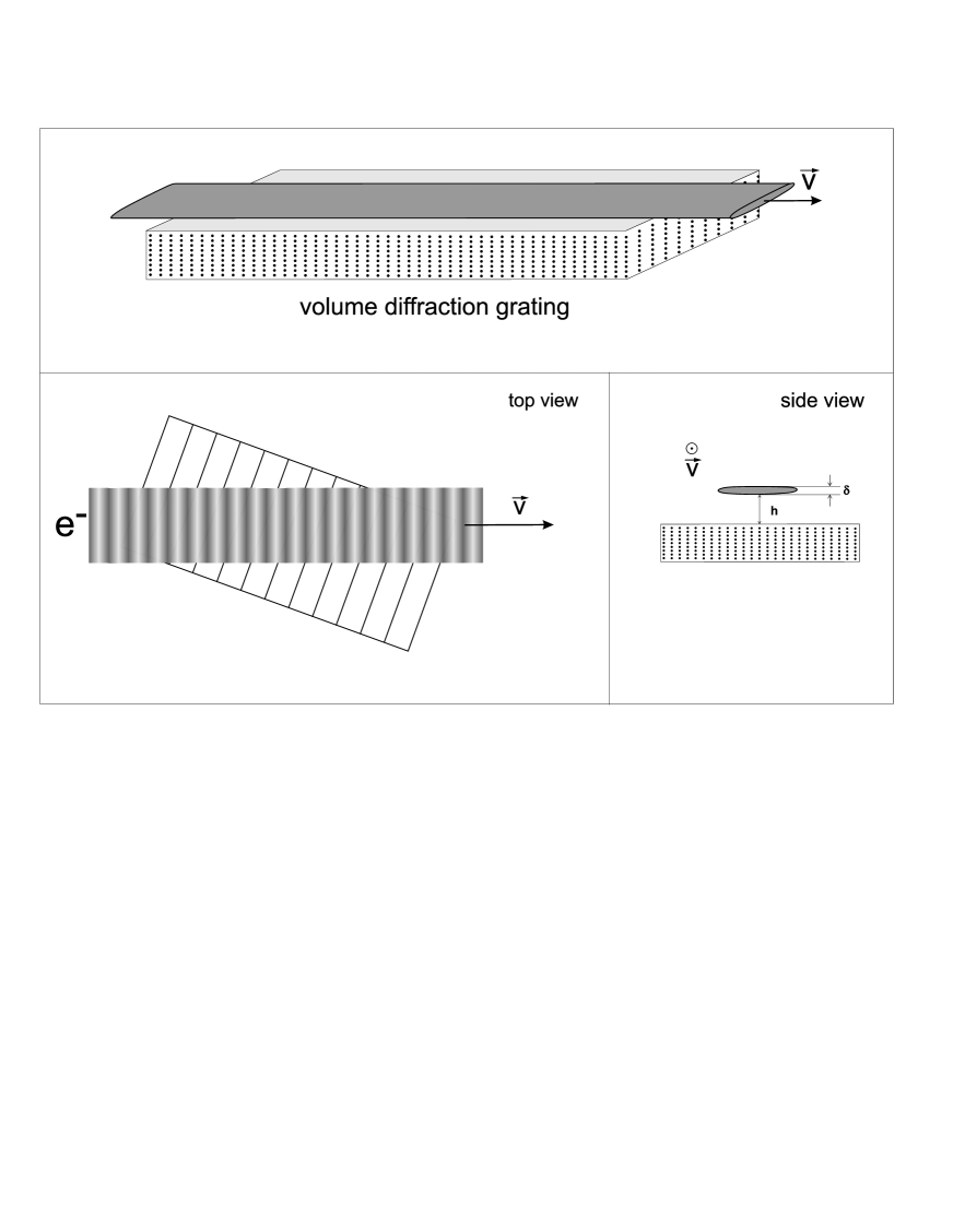
FIG. 1.: Electron beam is moving over the periodic structure

FIG. 2.: Dependence of dimensionless instability increment $\displaystyle\nu$ on the magnitude of guiding field ($\displaystyle a_{0}=\frac{eH_{0}}{mc\gamma\omega}$). The current density of electron beam is $\displaystyle j=10~{}A/cm^{2}$.

FIG. 3.: Dependence of dimensionless instability increment $\displaystyle\nu$ on the magnitude of guiding field ($\displaystyle a_{0}=\frac{eH_{0}}{mc\gamma\omega}$). The current density of electron beam is $\displaystyle j=100~{}A/cm^{2}$.

FIG. 4.: The contour plot for instability increment.The abscissa corresponds to $\displaystyle a_{0}$, the ordinate corresponds to current density $\displaystyle j~{}(A/cm^{2})$.

REFERENCES

• [1] P.A. Cherenkov. DAN SSSR. 2, 451 (1934).
• [2] V.G.Baryshevsky and I.D.Feranchuk, J. Physique. 44, 913 (1983).
• [3] S.J. Smith, E.M. Purcell, Phys. Rev. 92, 1069 (1953).
• [4] M.A. Piestrup, R.L.Finman, IEEE J. Quant. Electron. 19 (357).
• [5] V.G.Baryshevsky and I.D.Feranchuk, Phys.Letters. 102A,103 (1984).
• [6] V.G.Baryshevsky, K.G.Batrakov and I.Ya.Dubovskaya, J.Phys. D 24,1250 (1991).
• [7] V.G.Baryshevsky, K.G.Batrakov and I.Ya.Dubovskaya, Phys. Stat.Sol. 169 b, 235 (1992).
• [8] V.G.Baryshevsky, K.G.Batrakov and I.Ya.Dubovskaya, NIM, 341A, 274 (1994).
• [9] V.G.Baryshevsky, K.G.Batrakov, I.Ya.Dubovskaya, S.Sytova, NIM, 358A, 508 (1995).
• [10] V.G.Baryshevsky, K.G.Batrakov. $\displaystyle 21^{th}$ International FEL99 Conference Contributions http://www.desy.de/fel99/contributions/T05/M0-P-10.pdf, DESY, Hamburg, Germany 23,28 Aug. (1999).
Refer to caption