Information Theory and Learning:
A Physical Approach

Information Theory and Learning:
A Physical Approach
Ilya Mark Nemenman

a dissertation
presented to the faculty
of princeton university
in candidacy for the degree
of doctor of philosophy

recommended for acceptance
by the department of physics

November 2000

© Copyright 2024 by Ilya Mark Nemenman.
All rights reserved.

Abstract

We try to establish a unified information theoretic approach to learning and to explore some of its applications. First, we define predictive information as the mutual information between the past and the future of a time series, discuss its behavior as a function of the length of the series, and explain how other quantities of interest studied previously in learning theory—as well as in dynamical systems and statistical mechanics—emerge from this universally definable concept. We then prove that predictive information provides the unique measure for the complexity of dynamics underlying the time series and show that there are classes of models characterized by power–law growth of the predictive information that are qualitatively more complex than any of the systems that have been investigated before. Further, we investigate numerically the learning of a nonparametric probability density, which is an example of a problem with power–law complexity, and show that the proper Bayesian formulation of this problem provides for the ‘Occam’ factors that punish overly complex models and thus allow one to learn not only a solution within a specific model class, but also the class itself using the data only and with very few a priori assumptions. We study a possible information theoretic method that regularizes the learning of an undersampled discrete variable, and show that learning in such a setup goes through stages of very different complexities. Finally, we discuss how all of these ideas may be useful in various problems in physics, statistics, and, most importantly, biology.

Acknowledgements

Most importantly, I thank my family and my dearest friends; for if not for their wisdom, knowledge, love, and support I would never be who I am now. And I thank Bill Bialek, who is not just a perfect advisor, but a friend to me.

This thesis would not be what it is now if not for many, too many to name them all, people who mentored life and physics to me. So, in order of their appearance in my life I am grateful to Leonid Demikhovsky, Mikhail Polozov, Albert Minkevich, Valentin Rusak, people of the Department of Theoretical Physics at Belarusian State University, Betty Young, people of Santa Clara University, Gerald Fisher, Ronald Adler, people of the Physics and Astronomy Department at San Francisco State University, Anatoly Spitkovsky, Alexander Silbergleit, Gravity Probe B theory group, Curtis Callan, Vipul Periwal, the late Howard Stone, Alexander Polyakov, Olexei Motrunich, Akakii Melikidze, Stanislav Boldyrev, Sergei Gukov, Andrei Mikhailov, Timur Shutenko, people of the Department of Physics at Princeton University, Naftali Tishby, Gonzalo Garcia de Polavieja Embid, Methods in Computational Neuroscience course at Marine Biological Laboratory, Rob de Ruyter van Steveninck, Adrienne Fairhall, Jonathan Miller, Dmitry Rinberg, people of NEC Research Institute, and many others.

Thank you all!

Collaborators

This thesis is based on the work done in collaboration with William Bialek, Naftali Tishby, Adrienne Fairhall, and Jonathan Miller. In particular, Chapters 2 and 3 largely follow the papers by Bialek, Nemenman, and Tishby (2000), and Bialek and Nemenman (2000) respectively, and Chapter 4 is a part of the work in progress by Bialek, Fairhall, Miller, and Nemenman.

“All of the books in the world contain no more information than is broadcast as video in a single large American city in a single year. Not all bits have equal value.”

Carl Sagan

“My interest is in the future because I am going to spend the rest of my life there.”

Charles F. Kettering

“That is what learning is. You suddenly understand something you’ve understood all your life, but in a new way.”

Doris Lessing

“Learning is not compulsory$\dots$ Neither is survival.”

W. Edwards Deming

“Where is the knowledge we’ve lost in information?”

T. S. Eliot

“What most experimenters take for granted before they begin their experiments is infinitely more interesting than any results to which their experiments lead.”

Norbert Wiener

Chapter 1 Introduction: what do we know?

We hope that while reading this work our readers will unsurprisingly realize that they actually are learning something. However, what may come as a surprise is that they learn a lot more than they think: while reading this very sentence the photoreceptors in the eyes estimate the mean intensity of the ambient light and adapt to it; the auditory cortex monitors the surroundings and warns if a visitor knocks on the door. The reader skips the endings of some long, complicated words because he has already guessed what is coming; he then notices peculiarities in the stylistics of the text and soon learns to distinguish sentences written late at night. And then, finally, there is the “true” learning of the thoughts that the authors try to convey in their writing.

Learning is everywhere around and inside us, and it is absolutely essential for our second–to–second survival. In fact, because of its utmost importance and omnipresence each one of us has a well developed personal, unique intuition on what “learning” means, and how it works. One might think that such enormous experience would come in handy when studying learning from a scientific perspective, but the situation is quite the opposite: it is extremely difficult to build a theory that unites the enormous spectrum of possible learning problems. Intuition built up for the case of learning to play a musical instrument may be totally useless (and even destructive) for studying, for example, how we learn our first language, or master mathematical concepts. A multitude of ideas and approaches, each treating its specific problem and having only a slight relation to another, is indeed what we see in learning science now.

In fact, there even is no such thing as the “learning theory.” There is statistical learning theory, which builds probabilistic bounds on our ability to estimate the parameters of models that describe some observations, and its formalism seems completely disjoint from the designs of psychological and physiological experiments that study learning in humans and animals. Then there is the Minimal Description Length paradigm, which states that the shorter is the code for a set of samples, the better is the knowledge of the structure inside the samples; it is not clear how to connect these ideas to numerous learning curves defined in specific contexts of neural networks. Then there are ideas that since the speed or (conversely) the difficulty of learning is related intuitively to the complexity of the studied problem, learning and complexity should be studied together; this opens the Pandora box of different approaches to complexity (later in this work we list over a dozen of definitions of this quantity!) and does not even come close to quantifying learning and complexity of, say, some simple geometric concept. We can continue this list, but the point is clear. We believe that specific learning scenarios, however interesting and practical they may be, are not going to bring any more insight to our current understanding of learning (and, for that matter, complexity). What we need at this stage is not another example—there are too many of them to comprehend already—but a unifying, generalizing theory.

What do we expect from such a theory? We want it to be physical in its spirit. That is, it must explain and unify all accumulated knowledge of the subject (and thus necessarily have an element of a review), but this explanation should bring a new level of understanding to the old problems, a level from which all the problems appear as different realizations of one general phenomenon. However, explaining old data is just a half of a good theory. Using new tools we must also be able to ask and answer meaningful new questions, thus the theory should be constructive enough to serve as a kernel for development.

We build our presentation to address all of these questions. In Chapter 2 we introduce a version of the theory of learning and complexity which is built on information theory and the notion of predictability. After finishing the construction, we extensively analyze the literature to show that most of prior knowledge of the subject is subsumed in our more general approach. Then we try to show that the ideas do not only explain the old results but can be used to study new problems as well. For this, we discuss a broad spectrum of possible applications to physics, to computer science, and to biology, and then single out two examples for a detailed analysis. In Chapter 3 we study applications of our ideas to the learning of nonparametric continuous probability densities, and we show how complexity penalizing Occam factors work in this case. Then in Chapter 4 we turn to the seemingly easier problem of learning a probability distribution of a discrete variable, and we study how regularization based only on information theory makes learning possible in the undersampled regime.

One may argue that the examples we discuss are not enough to claim for certain that our theory indeed is constructive. We hope to resolve these fears in the nearest future by studying other possible applications that we mention throughout our work. However, we want to stress here explicitly that we believe that the theory itself is complete, the definitions that we make are sensible and unique, and the conclusions are general and universal.

Chapter 2 Predictability, Complexity, and Learning

2.1 Why study predictability?

There is an obvious interest in having practical algorithms for predicting the future, and there is a correspondingly large literature on the problem of time series extrapolation. But prediction is both more and less than extrapolation: we might be able to predict, for example, the chance of rain in the coming week even if we cannot extrapolate the trajectory of temperature fluctuations. In the spirit of its thermodynamic origins, information theory (Shannon 1948) characterizes the potentialities and limitations of all possible prediction algorithms, as well as unifying the analysis of extrapolation with the more general notion of predictability. Specifically, we can define a quantity—the predictive information—that measures how much our observations of the past can tell us about the future. The predictive information characterizes the world we are observing, and we shall see that this characterization is close to our intuition about the complexity of the underlying dynamics.

Prediction is one of the fundamental problems in neural computation. Much of what we admire in expert human performance is predictive in character—the point guard who passes the basketball to a place where his teammate will arrive in a split second, the chess master who knows how moves made now will influence the end game two hours hence, the investor who buys a stock in anticipation that it will grow in the year to come. More generally, we gather sensory information not for its own sake but in the hope that this information will guide our actions (including our verbal actions). But acting takes time, and sense data can guide us only to the extent that those data inform us about the state of the world at the time of our actions, so the only components of the incoming data that have a chance of being useful are those that are predictive. Put bluntly, nonpredictive information is useless to the organism, and it therefore makes sense to isolate the predictive information. It will turn out that most of the information we collect over a long period of time is nonpredictive, so that isolating the predictive information must go a long way toward separating out those features of the sensory world that are relevant for behavior.

One of the most important examples of prediction is the phenomenon of generalization in learning. Learning is formalized as finding a model that explains or describes a set of observations, but again this is useful precisely (and only) because we expect this model will continue to be valid: in the language of learning theory [see, for example, Vapnik (1998)] an animal can gain selective advantage not from its performance on the training data but only from its performance at generalization. Generalizing—and not “overfitting” the training data—is precisely the problem of isolating those features of the data that have predictive value (see also Bialek and Tishby, in preparation). Further, we know that the success of generalization hinges on controlling the complexity of the models that we are willing to consider as possibilities. Finally, learning a model to describe a data set can be seen as an encoding of those data, as emphasized by Rissanen (1989), and the quality of this encoding can be measured using the ideas of information theory. Thus the exploration of learning problems should provide us with explicit links among the concepts of entropy, predictability, and complexity.

The notion of complexity arises not only in learning theory, but also in several other contexts. Some physical systems exhibit more complex dynamics than others (turbulent vs. laminar flows in fluids), and some systems evolve toward more complex states than others (spin glasses vs. ferromagnets). The problem of characterizing complexity in physical systems has a substantial literature of its own [for an overview see Bennett (1990)]. In this context several authors have considered complexity measures based on entropy or mutual information, although as far as we know no clear connections have been drawn among the measures of complexity that arise in learning theory and those that arise in dynamical systems and statistical mechanics.

An essential difficulty in quantifying complexity is to distinguish complexity from randomness. A true random string cannot be compressed and hence requires a long description; it thus is complex in the sense defined by Kolmogorov (1965, Li and Vitányi 1993, Vitányi and Li 2000), yet the physical process that generates this string may have a very simple description. Both in statistical mechanics and in learning theory our intuitive notions of complexity correspond to the statements about complexity of the underlying process, and not directly to the description length or Kolmogorov complexity.

Our central result is that the predictive information provides a general measure of complexity which includes as special cases some relevant concepts from learning theory and from dynamical systems. While the work on the complexity of models in learning theory rests specifically on the idea that one is trying to infer a model from data, the predictive information is a property of the data (or, more precisely, of an ensemble of data) itself without reference to a specific class of underlying models. If the data are generated by a process in a known class but with unknown parameters, then we can calculate the predictive information explicitly and show that this information diverges logarithmically with the size of the data set we have observed; the coefficient of this divergence counts the number of parameters in the model, or more precisely the effective dimension of the model class, and this provides a link to known results of Rissanen and others. But our approach also allows us to quantify the complexity of processes that fall outside the finite dimensional models of conventional learning theory, and we show that these more complex processes are characterized by a power–law rather than a logarithmic divergence of the predictive information.

By analogy with the analysis of critical phenomena in statistical physics, the separation of logarithmic from power–law divergences, together with the measurement of coefficients and exponents for these divergences, allows us to define “universality classes” for the complexity of data streams. The power–law or nonparametric class of processes may be crucial in real world learning tasks, where the effective number of parameters becomes so large that asymptotic results for finitely parameterizable models are inaccessible in practice. There is empirical evidence that simple physical systems can generate dynamics in this complexity class, and there are hints that language also may fall in this class.

Finally, we argue that the divergent components of the predictive information provide a unique measure of complexity that is consistent with certain simple requirements. This argument is in the spirit of Shannon’s original derivation of entropy as the unique measure of available information. We believe that this uniqueness argument provides a conclusive answer to the question of how one should quantify the complexity of a process generating a time series.

With the evident cost of lengthening our discussion, we have tried to give a self–contained presentation that develops our point of view, uses simple examples to connect with known results, and then generalizes and goes beyond these results. Even in cases where at least the qualitative form of our results is known from previous work, we believe that our point of view elucidates some issues that may have been less the focus of earlier studies. Last but not least, we explore the possibilities for connecting our theoretical discussion with the experimental characterization of learning and complexity in neural systems.

2.2 A curious observation

Before starting the systematic analysis of the problem, we want to motivate our discussion further by presenting results of some simple numerical experiments. Suppose we have a 1-dimensional chain of Ising spins with the Hamiltonian given by

$$H=-\sum_{\rm i,j}J_{\rm ij}\sigma_{\rm i}\sigma_{\rm j},$$ (2.1)

where the matrix $J_{\rm ij}$ is not necessarily tridiagonal (that is, long range interactions are also allowed). One may identify spins pointing upwards with $1$ and downwards with $0$, and then a spin chain is equivalent to some sequence of binary digits. This sequence consists of (overlapping) words of $N$ digits each, $W_{\rm k}$, $k=0,1\cdots 2^{N}-1$. Even though there are $2^{N}$ such words total, they appear with very different frequencies $n(W_{k})$ in the spin chain [see Fig. (2.1) for details].

Figure 2.1: Calculating entropy of words of length $4$ in a chain of $17$ spins. For this chain, $n(W_{0})=n(W_{1})=n(W_{3})=n(W_{7})=n(W_{12})=n(W_{14})=2$, $n(W_{8})=n(W_{9})=1$, and all other frequencies are zero. Thus, $S(4)\approx 2.95\;{\rm bits}$.

If the number of spins is large, then counting these frequencies provides a good empirical estimate to $P_{N}(W_{k})$, the probability distribution of different words of length $N$. Then one can calculate the entropy $S(N)$ of this probability distribution by the usual formula

$$S(N)=-\sum_{k=0}^{2^{N}-1}P_{N}(W_{k})\log_{2}P_{N}(W_{k})\;\;\;\;\;\;{\rm(bits)}.$$ (2.2)

Since entropy is an extensive property, $S(N)$ is asymptotically proportional to $N$ for any spin chain. Choosing a different set of couplings $J_{\rm ij}$ may change the coefficient of proportionality (and finding this coefficient is usually the goal of statistical mechanics) but the linearity is never challenged.

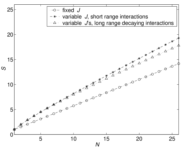
Figure 2.2: Entropy as a function of the word length for spin chains with different interactions. Notice that all lines start from $S(N)=\log_{2}2=1$ since at the values of the coupling we investigated the correlation length is much smaller than the chain length ($1\cdot 10^{9}$ spins).

We investigated this in three different spin chains of one billion spins each (the temperature is always $k_{B}T=1$). For the first chain, only $J_{\rm i,i+1}=1$ was nonzero, and its value was the same for all ${\rm i}$’s. The second chain was also generated using the nearest neighbor interactions, but the value of the coupling was reinitialized every 400,000 spins by taking a random number from a Gaussian distribution with a zero mean and a unit variance. In the third case, we again reinitialized at the same frequency, but now interactions were long–ranged, and the variance of coupling constants decreased with the distance between the spins as $\langle J_{\rm ij}^{2}\rangle=1/({\rm i}-{\rm j})^{2}$. We plotted $S(N)$ for all these cases in Fig. (2.2), and, of course, the asymptotically linear behavior seems to be evident—the extensive entropy shows no qualitative distinction between the three cases we consider.

However, the situation changes drastically if we remove the asymptotic linear contribution and plot only the sublinear component $S_{1}(N)$ of the entropy.

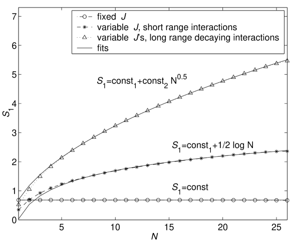
Figure 2.3: Subextensive part of the entropy as a function of the word length.

As we see in Fig. (2.3), the three investigated chains then exhibit qualitatively different features: for the first one, $S_{1}$ is constant; for the second one, it is logarithmic; and, for the third one, it clearly shows a power–law behavior.

What is the significance of this observation? Of course, the differences must be related to the ways we chose $J$’s for the simulations. In the first case, $J$ is fixed, and there is not much one can learn from observing the spin chain. For the second chain, $J$ changes, and the statistics of the spin–words is different in different parts of the sequence. By looking at this statistics, one can thus estimate coupling at the current position. Finally, in the third case there are many coupling constants that can be learned. In principle, as $N$ increases one becomes sensitive to correlations caused by interactions over larger and larger distances, and, since the variance of the couplings decays with the distance, interactions of longer range do not interfere with learning short–scale properties. So, intuitively, the qualitatively different behavior of $S_{1}(N)$ for the three plotted cases is due to a different character of learning tasks involved in understanding the spin chains. Much of this Chapter can be seen as expanding on and quantifying this intuitive observation.

2.3 Fundamentals

The problem of prediction comes in various forms, as noted above. Information theory allows us to treat the different notions of prediction on the same footing. The first step is to recognize that all predictions are probabilistic—even if we can predict the temperature at noon tomorrow, we should provide error bars or confidence limits on our prediction. The next step is to remember that, even before we look at the data, we know that certain futures are more likely than others, and we can summarize this knowledge by a prior probability distribution for the future. Our observations on the past lead us to a new, more tightly concentrated distribution, the distribution of futures conditional on the past data. Different kinds of predictions are different slices through or averages over this conditional distribution, but information theory quantifies the “concentration” of the distribution without making any commitment as to which averages will be most interesting.

Imagine that we observe a stream of data $x(t)$ over a time interval $-T<t<0$; let all of these past data be denoted by the shorthand $x_{\rm past}$. We are interested in saying something about the future, so we want to know about the data $x(t)$ that will be observed in the time interval $0<t<T^{\prime}$; let these future data be called $x_{\rm future}$. In the absence of any other knowledge, futures are drawn from the probability distribution $P(x_{\rm future})$, while observations of particular past data $x_{\rm past}$ tell us that futures will be drawn from the conditional distribution $P(x_{\rm future}|x_{\rm past})$. The greater concentration of the conditional distribution can be quantified by the fact that it has smaller entropy than the prior distribution, and this reduction in entropy is Shannon’s definition of the information that the past provides about the future. We can write the average of this predictive information as

$${\cal I}_{\rm pred}(T,T^{\prime}) = {\Bigg{\langle}}\log_{2}\left[{{P(x_{\rm future}|x_{\rm past})}\over{P(x_{\rm future})}}\right]\Bigg{\rangle}$$ (2.4)

$$= -\langle\log_{2}P(x_{\rm future})\rangle-\langle\log_{2}P(x_{\rm past})\rangle$$

$$\,\,\,\,\,\,\,\,\,\,-\left[-\langle\log_{2}P(x_{\rm future},x_{\rm past})\rangle\right]\,,$$

where $\langle\cdots\rangle$ denotes an average over the joint distribution of the past and the future, $P(x_{\rm future},x_{\rm past})$.

Each of the terms in Eq. (2.4) is an entropy. Since we are interested in predictability or generalization, which are associated with some features of the signal persisting forever, we may assume stationarity or invariance under time translations. Then the entropy of the past data depends only on the duration of our observations, so we can write $-\langle\log_{2}P(x_{\rm past})\rangle=S(T)$, and by the same argument $-\langle\log_{2}P(x_{\rm future})\rangle=S(T^{\prime})$. Finally, the entropy of the past and the future taken together is the entropy of observations on a window of duration $T+T^{\prime}$, so that $-\langle\log_{2}P(x_{\rm future},x_{\rm past})\rangle=S(T+T^{\prime})$. Putting these equations together, we obtain

$${\cal I}_{\rm pred}(T,T^{\prime})=S(T)+S(T^{\prime})-S(T+T^{\prime}).$$ (2.5)

In the same way that the entropy of a gas at fixed density is proportional to the volume, the entropy of a time series (asymptotically) is proportional to its duration, so that $\lim_{T\rightarrow\infty}{{S(T)}/T}={\cal S}_{0}$; entropy is an extensive quantity. But from Eq. (2.5) any extensive component of the entropy cancels in the computation of the predictive information: predictability is a deviation from extensivity. If we write $S(T)={\cal S}_{0}T+S_{1}(T)$, then Eq. (2.5) tells us that the predictive information is related only to the nonextensive term $S_{1}(T)$.

We know two general facts about the behavior of $S_{1}(T)$. First, the corrections to extensive behavior are positive, $S_{1}(T)\geq 0$. Second, the statement that entropy is extensive is the statement that the limit

$$\lim_{T\rightarrow\infty}{{S(T)}\over T}={\cal S}_{0}$$ (2.6)

exists, and for this to be true we must also have

$$\lim_{T\rightarrow\infty}{{S_{1}(T)}\over T}=0.$$ (2.7)

Thus the nonextensive terms in the entropy must be subextensive, that is they must grow with $T$ less rapidly than a linear function. Taken together, these facts guarantee that the predictive information is positive and subextensive. Further, if we let the future extend forward for a very long time, $T^{\prime}\rightarrow\infty$, then we can measure the information that our sample provides about the entire future,

$$I_{\rm pred}(T)=\lim_{T^{\prime}\rightarrow\infty}{\cal I}_{\rm pred}(T,T^{\prime})=S_{1}(T).$$ (2.8)

If we have been observing a time series for a (long) time $T$, then the total amount of data we have taken in is measured by the entropy $S(T)$, and at large $T$ this is given approximately by ${\cal S}_{0}T$. But the predictive information that we have gathered cannot grow linearly with time, even if we are making predictions about a future which stretches out to infinity. As a result, of the total information we have taken in by observing $x_{\rm past}$, only a vanishing fraction is of relevance to the prediction:

$$\lim_{T\rightarrow\infty}{{\rm Predictive\ Information}\over{\rm Total\ Information}}={{I_{\rm pred}(T)}\over{S(T)}}\rightarrow 0.$$ (2.9)

In this precise sense, most of what we observe is irrelevant to the problem of predicting the future. We can think of Eq. (2.9) as a law of diminishing returns: although we collect data in proportion to our observation time $T$, a smaller and smaller fraction of this information is useful in the problem of prediction. Note that these diminishing returns are not due to a limited lifetime, since we calculate the predictive information assuming that we have a future extending forward to infinity.

Now consider the case where time is measured in discrete steps, so that we have seen $N$ time points $x_{1},x_{2},\cdots,x_{N}$. How much have we learned about the underlying pattern in these data? The more we know, the more effectively we can predict the next data point $x_{N+1}$ and hence the fewer bits we will need to describe the deviation of this data point from our prediction: our accumulated knowledge about the time series is measured by the degree to which we can compress the description of new observations. On average, the length of the code word required to describe the point $x_{N+1}$, given that we have seen the previous $N$ points, is given by

$$\ell(N)=-\langle\log_{2}P(x_{N+1}|x_{1},x_{2},\cdots,x_{N})\rangle\,\,{\rm bits},$$ (2.10)

where the expectation value is taken over the joint distribution of all the $N+1$ points, $P(x_{1},x_{2},\cdots,x_{N},x_{N+1})$. It is easy to see that

$$\ell(N)=S(N+1)-S(N)\approx{{\partial S(N)}\over{\partial N}}.$$ (2.11)

As we observe for longer times, we learn more and this word length decreases. It is natural to define a learning curve that measures this improvement. Usually we define learning curves by measuring the frequency or costs of errors; here the cost is that our encoding of the point $x_{N+1}$ is longer than it could be if we had perfect knowledge. This ideal encoding has a length which we can find by imagining that we observe the time series for an infinitely long time, $\ell_{\rm ideal}=\lim_{N\rightarrow\infty}\ell(N)$, but this is just another way of defining the extensive component of the entropy ${\cal S}_{0}$. Thus we can define a learning curve

$$\Lambda(N) \equiv \ell(N)-\ell_{\rm ideal}$$

$$= S(N+1)-S(N)-{\cal S}_{0}$$

$$= S_{1}(N+1)-S_{1}(N)$$

$$\approx {{\partial S_{1}(N)}\over{\partial N}}={{\partial I_{\rm pred}(N)}\over{\partial N}},$$ (2.13)

and we see once again that the extensive component of the entropy cancels.

It is well known that the problems of prediction and compression are related, and what we have done here is to illustrate one aspect of this connection. Specifically, if we ask how much one segment of a time series can tell us about the future, the answer is contained in the subextensive behavior of the entropy. If we ask how much we are learning about the structure of the time series, then the natural and universally defined learning curve is related again to the subextensive entropy: the learning curve is the derivative of the predictive information.

This universal learning curve is connected to the more conventional learning curves in specific contexts. As an example (cf. Section 2.4.1), consider fitting a set of data points $\{x_{\rm n},y_{\rm n}\}$ with some class of functions $y=f(x;{\mbox{\boldmath$\alpha$}}),$ where the $\alpha$ are unknown parameters that need to be learned; we also allow for some Gaussian noise in our observation of the $y_{\rm n}$. Here the natural learning curve is the evolution of $\chi^{2}$ for generalization as a function of the number of examples. Within the approximations discussed below, it is straightforward to show that as $N$ becomes large,

$$\langle\chi^{2}(N)\rangle={1\over{\sigma^{2}}}\langle\left[y-f(x;{\mbox{\boldmath$\alpha$}})\right]^{2}\rangle\rightarrow 2\ln 2\,\Lambda(N)+1,$$ (2.14)

where $\sigma^{2}$ is the variance of the noise. Thus a more conventional measure of performance at learning a function is equal to the universal learning curve defined purely by information theoretic criteria. In other words, if a learning curve is measured in the right units, then its integral represents the amount of the useful information accumulated. Since one would expect any learning curve to decrease to zero eventually, we again obtain the ‘law of diminishing returns’.

Different quantities related to the subextensive entropy have been discussed in several contexts. For example, the code length $\ell(N)$ has been defined as a learning curve in the specific case of neural networks (Opper and Haussler 1995) and has been termed the “thermodynamic dive” (Crutchfield and Shalizi 1998) and “$N^{\rm th}$ order block entropy” (Grassberger 1986). Mutual information between all of the past and all of the future (both semi–infinite) is known also as the “excess entropy,” “effective measure complexity,” “stored information,” and so on [see Shalizi and Crutchfield (1999) and references therein, as well as the discussion below]. If the data allow a description by a model with a finite number of parameters, then mutual information between the data and the parameters is of interest, and this is also the predictive information about all of the future; some special cases of this problem have been discussed by Opper and Haussler (1995) and by Herschkowitz and Nadal (1999). What is important is that the predictive information or subextensive entropy is related to all these quantities, and that it can be defined for any process without a reference to a class of models. It is this universality that we find appealing, and this universality is strongest if we focus on the limit of long observation times. Qualitatively, in this regime ($T\rightarrow\infty$) we expect the predictive information to behave in one of three different ways: it may either stay finite, or grow to infinity together with $T$; in the latter case the rate of growth may be slow (logarithmic) or fast (sublinear power).

The first possibility, $\lim_{T\rightarrow\infty}I_{\rm pred}(T)=$ constant, means that no matter how long we observe we gain only a finite amount of information about the future. This situation prevails, for example, when the dynamics are too regular: for a purely periodic system, complete prediction is possible once we know the phase, and if we sample the data at discrete times this is a finite amount of information; longer period orbits intuitively are more complex and also have larger $I_{\rm pred}$, but this doesn’t change the limiting behavior $\lim_{T\rightarrow\infty}I_{\rm pred}(T)=$ constant.

Alternatively, the predictive information can be small when the dynamics are irregular but the best predictions are controlled only by the immediate past, so that the correlation times of the observable data are finite [see, for example, Crutchfield and Feldman (1997) and the fixed short–range interactions plot on Fig. (2.3)]. Imagine, for example, that we observe $x(t)$ at a series of discrete times $\{t_{\rm n}\}$, and that at each time point we find the value $x_{\rm n}$. Then we can always write the joint distribution of the $N$ data points as a product,

$$P(x_{1},x_{2},\cdots,x_{N}) = P(x_{1})P(x_{2}|x_{1})P(x_{3}|x_{2},x_{1})\cdots.$$ (2.15)

For Markov processes, what we observe at $t_{\rm n}$ depends only on events at the previous time step $t_{\rm n-1}$, so that

$$P(x_{\rm n}|\{x_{\rm 1\leq i\leq n-1}\}) = P(x_{\rm n}|x_{\rm n-1}),$$ (2.16)

and hence the predictive information reduces to

$$I_{\rm pred}=\Bigg{\langle}\log_{2}\left[{{P(x_{\rm n}|x_{\rm n-1})}\over{P(x_{\rm n})}}\right]\Bigg{\rangle}.$$ (2.17)

The maximum possible predictive information in this case is the entropy of the distribution of states at one time step, which in turn is bounded by the logarithm of the number of accessible states. To approach this bound the system must maintain memory for a long time, since the predictive information is reduced by the entropy of the transition probabilities. Thus systems with more states and longer memories have larger values of $I_{\rm pred}$.

More interesting are those cases in which $I_{\rm pred}(T)$ diverges at large $T$. In physical systems we know that there are critical points where correlation times become infinite, so that optimal predictions will be influenced by events in the arbitrarily distant past. Under these conditions the predictive information can grow without bound as $T$ becomes large; for many systems the divergence is logarithmic, $I_{\rm pred}(T\rightarrow\infty)\propto\ln T$, as for the variable $J_{\rm ij}$, short range Ising model of Figs. (2.2, 2.3). Long range correlation also are important in a time series where we can learn some underlying rules. It will turn out that when the set of possible rules can be described by a finite number of parameters, the predictive information again diverges logarithmically, and the coefficient of this divergence counts the number of parameters. Finally, a faster growth is also possible, so that $I_{\rm pred}(T\rightarrow\infty)\propto T^{\alpha}$, as for the variable $J_{\rm ij}$ long range Ising model, and we shall see that this behavior emerges from, for example, nonparametric learning problems.

2.4 Learning and predictability

Learning is of interest precisely in those situations where correlations or associations persist over long periods of time. In the usual theoretical models, there is some rule underlying the observable data, and this rule is valid forever; examples seen at one time inform us about the rule, and this information can be used to make predictions or generalizations. The predictive information quantifies the average generalization power of examples, and we shall see that there is a direct connection between the predictive information and the complexity of the possible underlying rules.

2.4.1 A test case

Let us begin with a simple example already mentioned above. We observe two streams of data $x$ and $y$, or equivalently a stream of pairs $(x_{\rm 1},y_{\rm 1})$, $(x_{\rm 2},y_{\rm 2})$, $\cdots$ , $(x_{\rm N},y_{\rm N})$. Assume that we know in advance that the $x$’s are drawn independently and at random from some distribution $P(x)$, while the $y$’s are noisy versions of some function acting on $x$,

$$y_{\rm n}=f(x_{\rm n};{\mbox{\boldmath$\alpha$}})+\eta_{\rm n},$$ (2.18)

where $f(x;{\mbox{\boldmath$\alpha$}})$ is a class of functions parameterized by $\alpha$, and $\eta_{\rm n}$ is some noise which for simplicity we will assume is Gaussian with some known standard deviation $\sigma$. We can even start with a very simple case, where the function class is just a linear combination of some basis functions, so that

$$f(x;{\mbox{\boldmath$\alpha$}})=\sum_{\rm\mu=1}^{K}\alpha_{\mu}\phi_{\mu}(x).$$ (2.19)

The usual problem is to estimate, from $N$ pairs $\{x_{\rm i},y_{\rm i}\}$, the values of the parameters $\alpha$; in favorable cases such as this we might even be able to find an effective regression formula. We are interested in evaluating the predictive information, which means that we need to know the entropy $S(N)$. We go through the calculation in some detail because it provides a model for the more general case.

To evaluate the entropy $S(N)$ we first construct the probability distribution $P(x_{\rm 1},y_{\rm 1},x_{\rm 2},y_{\rm 2},\cdots,x_{\rm N},y_{\rm N})$. The same set of rules apply to the whole data stream, which here means that the same parameters $\alpha$ apply for all pairs $\{x_{\rm i},y_{\rm i}\}$, but these parameters are chosen at random from a distribution ${\cal P}({\mbox{\boldmath$\alpha$}})$ at the start of the stream. Thus we write

$$P(x_{\rm 1},y_{\rm 1},x_{\rm 2},y_{\rm 2},\cdots,x_{\rm N},y_{\rm N})$$

$$\,\,\,\,\,=\int d^{K}\alpha\,P(x_{\rm 1},y_{\rm 1},x_{\rm 2},y_{\rm 2},\cdots,x_{\rm N},y_{\rm N}|{\mbox{\boldmath$\alpha$}}){\cal P}({\mbox{\boldmath$\alpha$}})\,,$$ (2.20)

and now we need to construct the conditional distributions for fixed $\alpha$. By hypothesis each $x$ is chosen independently, and once we fix $\alpha$ each $y_{\rm i}$ is correlated only with the corresponding $x_{\rm i}$, so that we have

$$P(x_{\rm 1},y_{\rm 1},x_{\rm 2},y_{\rm 2},\cdots,x_{\rm N},y_{\rm N}|{\mbox{\boldmath$\alpha$}})=\prod_{\rm i=1}^{\rm N}\left[P(x_{\rm i})\,P(y_{\rm i}|x_{\rm i};{\mbox{\boldmath$\alpha$}})\right]\,.$$ (2.21)

Further, with the simple assumptions above about the class of functions and Gaussian noise, the conditional distribution of $y_{\rm i}$ has the form

$$P(y_{\rm i}|x_{\rm i};{\mbox{\boldmath$\alpha$}})={1\over\sqrt{2\pi\sigma^{2}}}\exp\left[-{1\over{2\sigma^{2}}}\left(y_{\rm i}-\sum_{\mu=1}^{K}\alpha_{\mu}\phi_{\mu}(x_{\rm i})\right)^{2}\right]\,.$$ (2.22)

Putting all these factors together,

$$P(x_{\rm 1},y_{\rm 1},x_{\rm 2},y_{\rm 2},\cdots,x_{\rm N},y_{\rm N})$$

$$\,\,\,\,\,=\left[\prod_{\rm i=1}^{\rm N}P(x_{\rm i})\right]\left({1\over\sqrt{2\pi\sigma^{2}}}\right)^{N}\int d^{K}\alpha\,{\cal P}({\mbox{\boldmath$\alpha$}})\exp\left[-{1\over{2\sigma^{2}}}\sum_{\rm i=1}^{\rm N}y_{\rm i}^{2}\right]$$

$$\,\,\,\,\,\,\,\,\,\,\times\exp\left[-{N\over 2}\sum_{\mu,\nu=1}^{K}A_{\mu\nu}(\{x_{\rm i}\})\alpha_{\mu}\alpha_{\nu}+N\sum_{\mu=1}^{K}B_{\mu}(\{x_{\rm i},y_{\rm i}\})\alpha_{\mu}\right],$$ (2.23)

where

$$A_{\mu\nu}(\{x_{\rm i}\}) = {1\over{\sigma^{2}N}}\sum_{\rm i=1}^{\rm N}\phi_{\mu}(x_{\rm i})\phi_{\nu}(x_{\rm i}),\,\,\,\,{\rm and}$$ (2.24)

$$B_{\mu}(\{x_{\rm i},y_{\rm i}\}) = {1\over{\sigma^{2}N}}\sum_{\rm i=1}^{\rm N}y_{\rm i}\phi_{\mu}(x_{\rm i}).$$ (2.25)

Our placement of the factors of $N$ means that both $A_{\mu\nu}$ and $B_{\mu}$ are of order unity as $N\rightarrow\infty$. These quantities are empirical averages over the samples $\{x_{\rm i},y_{\rm i}\}$, and if the $\phi_{\mu}$ are well behaved we expect that these empirical means converge to expectation values for most realizations of the series $\{x_{\rm i}\}$:

$$\lim_{N\rightarrow\infty}A_{\mu\nu}(\{x_{\rm i}\}) = A_{\mu\nu}^{\infty}={1\over{\sigma^{2}}}\int dxP(x)\phi_{\mu}(x)\phi_{\nu}(x)\,,$$ (2.26)

$$\lim_{N\rightarrow\infty}B_{\mu}(\{x_{\rm i},y_{\rm i}\}) = B_{\mu}^{\infty}=\sum_{\nu=1}^{K}A_{\mu\nu}^{\infty}\bar{\alpha}_{\nu}\,,$$ (2.27)

where $\bar{\mbox{\boldmath$\alpha$}}$ are the parameters that actually gave rise to the data stream $\{x_{\rm i},y_{\rm i}\}$. In fact we can make the same argument about the terms in $\sum y_{\rm i}^{2}$,

$$\lim_{N\rightarrow\infty}\sum_{\rm i=1}^{\rm N}y_{\rm i}^{2}=N\sigma^{2}\left[\sum_{\mu,\nu=1}^{K}{\bar{\alpha}}_{\mu}A_{\mu\nu}^{\infty}{\bar{\alpha}}_{\nu}+1\right].$$ (2.28)

Conditions for this convergence of empirical means to expectation values are at the heart of learning theory. Our approach here is first to assume that this convergence works, then to examine the consequences for the predictive information, and finally to address the conditions for and implications of this convergence breaking down.

Putting the different factors together, we obtain

$$P(x_{\rm 1},y_{\rm 1},x_{\rm 2},y_{\rm 2},\cdots,x_{\rm N},y_{\rm N})$$

$$\,\,\,\,\,{\widetilde{\rightarrow}}\left[\prod_{\rm i=1}^{\rm N}P(x_{\rm i})\right]\left({1\over\sqrt{2\pi\sigma^{2}}}\right)^{N}\int d^{K}\alpha{\cal P}({\mbox{\boldmath$\alpha$}})\exp\left[-NE_{N}({\mbox{\boldmath$\alpha$}};\{x_{\rm i},y_{\rm i}\})\right],$$

where the effective “energy” per sample is given by

$$E_{N}({\mbox{\boldmath$\alpha$}};\{x_{\rm i},y_{\rm i}\})={1\over 2}+{1\over 2}\sum_{\mu,\nu=1}^{K}(\alpha_{\mu}-{\bar{\alpha}}_{\mu})A_{\mu\nu}^{\infty}(\alpha_{\nu}-{\bar{\alpha}}_{\nu}).$$ (2.30)

Here we use the symbol ${\widetilde{\to}}$ to indicate that we not only take the limit of large $N$, but also neglect the fluctuations. Note that in this approximation the dependence on the sample points themselves is hidden in the definition of $\bar{\mbox{\boldmath$\alpha$}}$ as being the parameters that generated the samples.

The integral that we need to do in Eq. (2.4.1) involves an exponential with a large factor $N$ in the exponent; the free energy $F_{N}$ is of order unity as $N\rightarrow\infty$. This suggests that we evaluate the integral by a saddle point or steepest descent approximation [similar analyses were performed by Clarke and Barron (1990), by MacKay (1992), and by Balasubramanian (1997)]:

$$\int d^{K}\alpha{\cal P}({\mbox{\boldmath$\alpha$}})\exp\left[-NE_{N}({\mbox{\boldmath$\alpha$}};\{x_{\rm i},y_{\rm i}\})\right]\approx{\cal P}({\mbox{\boldmath$\alpha$}}_{\rm cl})$$

$$\,\,\,\,\times\exp\left[-NE_{N}({\mbox{\boldmath$\alpha$}}_{\rm cl};\{x_{\rm i},y_{\rm i}\})-{K\over 2}\ln{N\over{2\pi}}-{1\over 2}\ln\det{\cal F}_{N}+\cdots\right],$$ (2.31)

where ${\mbox{\boldmath$\alpha$}}_{\rm cl}$ is the “classical” value of $\alpha$ determined by the extremal conditions

$${{\partial E_{N}({\mbox{\boldmath$\alpha$}};\{x_{\rm i},y_{\rm i}\})}\over{\partial\alpha_{\mu}}}\Bigg{|}_{{\mbox{\boldmath$\alpha$}}={\mbox{\boldmath$\alpha$}}_{\rm cl}}=0,$$ (2.32)

the matrix ${\cal F}_{N}$ consists of the second derivatives of $E_{N}$,

$${\cal F}_{N}={{\partial^{2}E_{N}({\mbox{\boldmath$\alpha$}};\{x_{\rm i},y_{\rm i}\})}\over{\partial\alpha_{\mu}\partial\alpha_{\nu}}}\Bigg{|}_{{\mbox{\boldmath$\alpha$}}={\mbox{\boldmath$\alpha$}}_{\rm cl}},$$ (2.33)

and $\cdots$ denotes terms that vanish as $N\rightarrow\infty$. If we formulate the problem of estimating the parameters $\alpha$ from the samples $\{x_{\rm i},y_{\rm i}\}$, then as $N\rightarrow\infty$ the matrix $N{\cal F}_{N}$ is the Fisher information matrix (Cover and Thomas 1991); the eigenvectors of this matrix give the principal axes for the error ellipsoid in parameter space, and the (inverse) eigenvalues give the variances of parameter estimates along each of these directions. The classical ${\mbox{\boldmath$\alpha$}}_{\rm cl}$ differs from $\bar{\mbox{\boldmath$\alpha$}}$ only in terms of order $1/N$; we neglect this difference and further simplify the calculation of leading terms as $N$ becomes large. After a little more algebra, then, we find the probability distribution we have been looking for:

$$P(x_{\rm 1},y_{\rm 1},x_{\rm 2},y_{\rm 2},\cdots,x_{\rm N},y_{\rm N})$$

$$\,\,\,\,\,\widetilde{\rightarrow}\left[\prod_{\rm i=1}^{\rm N}P(x_{\rm i})\right]{1\over{Z_{A}}}{\cal P}(\bar{\mbox{\boldmath$\alpha$}})\exp\left[-{N\over 2}\ln(2\pi{\rm e}\sigma^{2})-{K\over 2}\ln N+\cdots\right],$$ (2.34)

where the normalization constant

$${Z_{A}}=\sqrt{(2\pi)^{K}\det A^{\infty}}.$$ (2.35)

Again we note that the sample points $\{x_{\rm i},y_{\rm i}\}$ are hidden in the value of $\bar{\mbox{\boldmath$\alpha$}}$ that gave rise to these points.

To evaluate the entropy $S(N)$ we need to compute the expectation value of the (negative) logarithm of the probability distribution in Eq. (2.34); there are three terms. One is constant, so averaging is trivial. The second term depends only on the $x_{\rm i}$, and because these are chosen independently from the distribution $P(x)$ the average again is easy to evaluate. The third term involves $\bar{\mbox{\boldmath$\alpha$}}$, and we need to average this over the joint distribution $P(x_{\rm 1},y_{\rm 1},x_{\rm 2},y_{\rm 2},\cdots,x_{\rm N},y_{\rm N})$. As above, we can evaluate this average in steps: first we choose a value of the parameters $\bar{\mbox{\boldmath$\alpha$}}$, then we average over the samples given these parameters, and finally we average over parameters. But because $\bar{\mbox{\boldmath$\alpha$}}$ is defined as the parameters that generate the samples, this stepwise procedure simplifies enormously. The end result is that

$$S(N)=N\left[S_{x}+{1\over 2}\log_{2}(2\pi{\rm e}\sigma^{2})\right]+{K\over 2}\log_{2}N+S_{\mbox{{\scriptsize\boldmath$\alpha$}}}+\langle\log_{2}{Z_{A}}\rangle_{\mbox{{\scriptsize\boldmath$\alpha$}}}+\cdots,$$ (2.36)

where $\langle\cdots\rangle_{\mbox{{\scriptsize\boldmath$\alpha$}}}$ means averaging over parameters, $S_{x}$ is the entropy of the distribution of $x$,

$$S_{x}=-\int dx\,P(x)\log_{2}P(x),$$ (2.37)

and similarly for the entropy of the distribution of parameters,

$$S_{\mbox{{\scriptsize\boldmath$\alpha$}}}=-\int d^{K}\alpha\,{\cal P}({\mbox{\boldmath$\alpha$}})\log_{2}{\cal P}({\mbox{\boldmath$\alpha$}}).$$ (2.38)

The different terms in the entropy Eq. (2.36) have a straightforward interpretation. First we see that the extensive term in the entropy,

$${\cal S}_{0}=S_{x}+{1\over 2}\log_{2}(2\pi{\rm e}\sigma^{2}),$$ (2.39)

reflects contributions from the random choice of $x$ and from the Gaussian noise in $y$; these extensive terms are independent of the variations in parameters $\alpha$, and these would be the only terms if the parameters were not varying (that is, if there were nothing to learn). There also is a term which reflects the entropy of variations in the parameters themselves, $S_{\mbox{{\scriptsize\boldmath$\alpha$}}}$. This entropy is not invariant with respect to coordinate transformations in the parameter space, but the term $\langle\log_{2}Z_{A}\rangle_{\mbox{{\scriptsize\boldmath$\alpha$}}}$ compensates for this noninvariance. Finally, and most interestingly for our purposes, the subextensive piece of the entropy is dominated by a logarithmic divergence,

$$S_{1}(N)\rightarrow{K\over 2}\log_{2}N\;\;\;{\rm(bits)}.$$ (2.40)

The coefficient of this divergence counts the number of parameters independent of the coordinate system that we choose in the parameter space. Furthermore, this result does not depend on the set of basis functions $\{\phi_{\mu}(x)\}$. This is a hint that the result in Eq. (2.40) is more universal than our simple example.

2.4.2 Learning a parameterized distribution

The problem discussed above is an example of supervised learning: we are given examples of how the points $x_{\rm n}$ map into $y_{\rm n}$, and from these examples we are to induce the association or functional relation between $x$ and $y$. An alternative view is that pair of points $(x,y)$ should be viewed as a vector $\vec{x}$, and what we are learning is the distribution of this vector. The problem of learning a distribution usually is called unsupervised learning, but in this case supervised learning formally is a special case of unsupervised learning; if we admit that all the functional relations or associations that we are trying to learn have an element of noise or stochasticity, then this connection between supervised and unsupervised problems is quite general.

Suppose a series of random vector variables $\{{\vec{x}}_{\rm i}\}$ are drawn independently from the same probability distribution $Q({\vec{x}}|{\mbox{\boldmath$\alpha$}})$, and this distribution depends on a (potentially infinite dimensional) vector of parameters $\alpha$. As above, the parameters are unknown, and before the series starts they are chosen randomly from a distribution ${\cal P}(\mbox{\boldmath$\alpha$})$. With no constraints on the densities ${\cal P}(\mbox{\boldmath$\alpha$})$ or $Q({\vec{x}}|{\mbox{\boldmath$\alpha$}})$ it is impossible to derive any regression formulas for parameter estimation, but one can still calculate the leading terms in the entropy of the data series and thus the predictive information.

We begin with the definition of entropy

$$S(N)\equiv S[\left\{\vec{x}_{\rm i}\right\}]=-\int d{\vec{x}}_{\rm 1}\cdots d{\vec{x}}_{\rm N}\,P({\vec{x}}_{\rm 1},{\vec{x}}_{\rm 2},\cdots,{\vec{x}}_{\rm N})\,\log_{2}P({\vec{x}}_{\rm 1},{\vec{x}}_{\rm 2},\cdots,{\vec{x}}_{\rm N}).$$ (2.41)

By analogy with Eq. (2.20) we then write

$$P({\vec{x}}_{\rm 1},{\vec{x}}_{\rm 2},\cdots,{\vec{x}}_{\rm N})=\int d^{K}\alpha{\cal P}({\mbox{\boldmath$\alpha$}})\prod_{\rm i=1}^{\rm N}Q({\vec{x}}_{\rm i}|{\mbox{\boldmath$\alpha$}}).$$ (2.42)

Next, combining the last two equations and rearranging the order of integration, we can rewrite $S(N)$ as

$$S(N) = -\int d^{K}\bar{\mbox{\boldmath$\alpha$}}{\cal P}(\bar{\mbox{\boldmath$\alpha$}})\left\{\int d{\vec{x}}_{\rm 1}\cdots d{\vec{x}}_{\rm N}\,\prod_{\rm j=1}^{\rm N}Q({\vec{x}}_{\rm j}|\bar{\mbox{\boldmath$\alpha$}})\;\log_{2}P(\{{\vec{x}}_{\rm i}\})\right\}.$$ (2.43)

Eq. (2.43) allows an easy interpretation. There is the ‘true’ set of parameters $\bar{\mbox{\boldmath$\alpha$}}$ that gave rise to the data sequence ${\vec{x}}_{\rm 1}\cdots{\vec{x}}_{\rm N}$ with the probability $\prod_{\rm j=1}^{\rm N}Q({\vec{x}}_{\rm j}|\bar{\mbox{\boldmath$\alpha$}})$. We need to average $\log_{2}P({\vec{x}}_{\rm 1}\cdots{\vec{x}}_{\rm N})$ first over all possible realizations of the data keeping the true parameters fixed, and then over the parameters $\bar{\mbox{\boldmath$\alpha$}}$ themselves. With this interpretation in mind, the joint probability density, the logarithm of which is being averaged, can be rewritten in the following useful way:

$$P({\vec{x}}_{\rm 1},\cdots,{\vec{x}}_{\rm N}) = \prod_{\rm j=1}^{\rm N}Q({\vec{x}}_{\rm j}|\bar{\mbox{\boldmath$\alpha$}})\int d^{K}\alpha{\cal P}({\mbox{\boldmath$\alpha$}})\prod_{\rm i=1}^{\rm N}\left[{{Q({\vec{x}}_{\rm i}|{\mbox{\boldmath$\alpha$}})}\over{Q({\vec{x}}_{\rm i}|\bar{\mbox{\boldmath$\alpha$}})}}\right]$$ (2.44)

$$= \prod_{\rm j=1}^{\rm N}Q({\vec{x}}_{\rm j}|\bar{\mbox{\boldmath$\alpha$}})\int d^{K}\alpha{\cal P}({\mbox{\boldmath$\alpha$}})\exp\left[-N{\cal E}_{N}({\mbox{\boldmath$\alpha$}};\{{\vec{x}}_{\rm i}\})\right],$$

$${\cal E}_{N}({\mbox{\boldmath$\alpha$}};\{{\vec{x}}_{\rm i}\}) = -{1\over N}\sum_{\rm i=1}^{\rm N}\ln\left[{{Q({\vec{x}}_{\rm i}|{\mbox{\boldmath$\alpha$}})}\over{Q({\vec{x}}_{\rm i}|\bar{\mbox{\boldmath$\alpha$}})}}\right].$$ (2.45)

Since, by our interpretation, $\bar{\mbox{\boldmath$\alpha$}}$ are the true parameters that gave rise to the particular data $\{{\vec{x}}_{\rm i}\}$, we may expect empirical means to converge to expectation values, so that

$${\cal E}_{N}({\mbox{\boldmath$\alpha$}};\{{\vec{x}}_{\rm i}\})=-\int d^{D}xQ(x|\bar{\mbox{\boldmath$\alpha$}})\ln\left[{{Q({\vec{x}}|{\mbox{\boldmath$\alpha$}})}\over{Q({\vec{x}}|\bar{\mbox{\boldmath$\alpha$}})}}\right]-\psi({\mbox{\boldmath$\alpha$}},\bar{\mbox{\boldmath$\alpha$}};\{x_{\rm i}\}),$$ (2.46)

where $\psi\rightarrow 0$ as $N\rightarrow\infty$; here we neglect $\psi$, and return to this term below.

The first term on the right hand side of Eq. (2.46) is the Kullback–Leibler divergence, $D_{\rm KL}({\mbox{\boldmath$\bar{\alpha}$}}||{\mbox{\boldmath$\alpha$}})$, between the true distribution characterized by parameters $\bar{\mbox{\boldmath$\alpha$}}$ and the possible distribution characterized by $\alpha$. Thus at large $N$ we have

$$P({\vec{x}}_{\rm 1},{\vec{x}}_{\rm 2},\cdots,{\vec{x}}_{\rm N})\widetilde{\rightarrow}\prod_{\rm j=1}^{\rm N}Q({\vec{x}}_{\rm j}|\bar{\mbox{\boldmath$\alpha$}})\int d^{K}\alpha{\cal P}({\mbox{\boldmath$\alpha$}})\exp\left[-ND_{\rm KL}(\bar{\mbox{\boldmath$\alpha$}}||{\mbox{\boldmath$\alpha$}})\right],$$ (2.47)

where again the notation $\widetilde{\rightarrow}$ reminds us that we are not only taking the limit of large $N$ but also making another approximation in neglecting fluctuations. By the same arguments as above we can proceed (formally) to compute the entropy of this distribution, and we find

$$S(N) \approx {\cal S}_{0}\cdot N+S^{({\rm a})}_{1}(N),$$ (2.48)

$${\cal S}_{0} = \int d^{K}\alpha{\cal P}({\mbox{\boldmath$\alpha$}})\left[-\int d^{D}xQ({\vec{x}}|{\mbox{\boldmath$\alpha$}})\log_{2}Q({\vec{x}}|{\mbox{\boldmath$\alpha$}})\right],\,\,\,\,{\rm and}$$ (2.49)

$$S^{({\rm a})}_{1}(N) = -\int d^{K}{\bar{\alpha}}{\cal P}(\bar{\mbox{\boldmath$\alpha$}})\log_{2}\left[\int d^{K}\alpha P({\mbox{\boldmath$\alpha$}}){\rm e}^{-ND_{\rm KL}(\bar{\mbox{{\scriptsize\boldmath$\alpha$}}}||{\mbox{{\scriptsize\boldmath$\alpha$}}})}\right].$$ (2.50)

Here $S^{({\rm a})}_{1}$ is an approximation to $S_{1}$ that neglects fluctuations $\psi$. This is the same as the annealed approximation in the statistical mechanics of disordered systems, as has been used widely in the study of supervised learning problems (Seung et al. 1992). Thus we can identify the data sequence ${\vec{x}}_{\rm 1}\cdots{\vec{x}}_{\rm N}$ with the disorder, ${\cal E}_{N}({\mbox{\boldmath$\alpha$}};\{{\vec{x}}_{\rm i}\})$ with the energy of the quenched system, and $D_{\rm KL}(\bar{\mbox{\boldmath$\alpha$}}||{\mbox{\boldmath$\alpha$}})$ with its annealed analogue.

The extensive term ${\cal S}_{0}$, Eq. (2.49), is the average entropy of a distribution in our family of possible distributions, generalizing the result of Eq. (2.39). The subextensive terms in the entropy are controlled by the $N$ dependence of the partition function

$$Z({\bar{\mbox{\boldmath$\alpha$}}};N)=\int d^{K}\alpha{\cal P}({\mbox{\boldmath$\alpha$}})\exp\left[-ND_{\rm KL}(\bar{\mbox{\boldmath$\alpha$}}||{\mbox{\boldmath$\alpha$}})\right],$$ (2.51)

and $S_{1}(N)=-\langle\log_{2}Z({\bar{\mbox{\boldmath$\alpha$}}};N)\rangle_{\bar{\mbox{{\scriptsize\boldmath$\alpha$}}}}$ is analogous to the free energy. Since what is important in this integral is the Kullback–Leibler (KL) divergence between different distributions, it is natural to ask about the density of models that are KL divergence $D$ away from the target $\bar{\mbox{\boldmath$\alpha$}}$,

$$\rho(D;{\bar{\mbox{\boldmath$\alpha$}}})=\int d^{K}\alpha{\cal P}({\mbox{\boldmath$\alpha$}})\delta[D-D_{\rm KL}(\bar{\mbox{\boldmath$\alpha$}}||{\mbox{\boldmath$\alpha$}})];$$ (2.52)

note that this density could be very different for different targets. The density of divergences is normalized because the original distribution over parameter space, $P({\mbox{\boldmath$\alpha$}})$, is normalized,

$$\int dD\rho(D;{\bar{\mbox{\boldmath$\alpha$}}})=\int d^{K}\alpha{\cal P}({\mbox{\boldmath$\alpha$}})=1.$$ (2.53)

Finally, the partition function takes the simple form

$$Z({\bar{\mbox{\boldmath$\alpha$}}};N)=\int dD\rho(D;{\bar{\mbox{\boldmath$\alpha$}}})\exp[-ND].$$ (2.54)

We recall that in statistical mechanics the partition function is given by

$$Z(\beta)=\int dE\rho(E)\exp[-\beta E],$$ (2.55)

where $\rho(E)$ is the density of states that have energy $E$, and $\beta$ is the inverse temperature. Thus the subextensive entropy in our learning problem is analogous to a system in which energy corresponds to the Kullback–Leibler divergence relative to the target model, and temperature is inverse to the number of examples. As we increase the length $N$ of the time series we have observed, we “cool” the system and hence probe models which approach the target; the dynamics of this approach is determined by the density of low energy states, that is the behavior of $\rho(D;{\bar{\mbox{\boldmath$\alpha$}}})$ as $D\rightarrow 0$.

The structure of the partition function is determined by a competition between the (Boltzmann) exponential term, which favors models with small $D$, and the density term, which favors values of $D$ that can be achieved by the largest possible number of models. Because there (typically) are many parameters, there are very few models with $D\rightarrow 0$. This picture of competition between the Boltzmann factor and a density of states has been emphasized in previous work on supervised learning (Haussler et al. 1996).

The behavior of the density of states, $\rho(D;{\bar{\mbox{\boldmath$\alpha$}}})$, at small $D$ is related to the more intuitive notion of dimensionality. In a parameterized family of distributions, the Kullback–Leibler divergence between two distributions with nearby parameters is approximately a quadratic form,

$$D_{\rm KL}(\bar{\mbox{\boldmath$\alpha$}}||{\mbox{\boldmath$\alpha$}})\approx{1\over 2}\sum_{\mu\nu}(\bar{\alpha}_{\mu}-\alpha_{\mu}){\cal F}_{\mu\nu}(\bar{\alpha}_{\nu}-\alpha_{\nu})+\cdots,$$ (2.56)

where ${\cal F}$ is the Fisher information matrix. Intuitively, if we have a reasonable parameterization of the distributions, then similar distributions will be nearby in parameter space, and more importantly points that are far apart in parameter space will never correspond to similar distributions; Clarke and Barron (1990) refer to this condition as the parameterization forming a “sound” family of distributions. If this condition is obeyed, then we can approximate the low $D$ limit of the density $\rho(D;{\bar{\mbox{\boldmath$\alpha$}}})$:

$$\rho(D;{\bar{\mbox{\boldmath$\alpha$}}}) = \int d^{K}\alpha{\cal P}({\mbox{\boldmath$\alpha$}})\delta[D-D_{\rm KL}(\bar{\mbox{\boldmath$\alpha$}}||{\mbox{\boldmath$\alpha$}})]$$ (2.57)

$$\approx \int d^{K}\alpha{\cal P}({\mbox{\boldmath$\alpha$}})\delta\left[D-{1\over 2}\sum_{\mu\nu}(\bar{\alpha}_{\mu}-\alpha_{\mu}){\cal F}_{\mu\nu}(\bar{\alpha}_{\nu}-\alpha_{\nu})\right]$$

$$= \int d^{K}\alpha{\cal P}(\bar{\mbox{\boldmath$\alpha$}}+{\cal U}\cdot{\mbox{\boldmath$\xi$}})\delta\left[D-{1\over 2}\sum_{\mu}\Lambda_{\mu}\xi_{\mu}^{2}\right],$$

where $\cal U$ is a matrix that diagonalizes $\cal F$,

$$({\cal U}^{T}\cdot{\cal F}\cdot{\cal U})_{\mu\nu}=\Lambda_{\mu}\delta_{\mu\nu}.$$ (2.58)

The delta function restricts the components of $\xi$ in Eq. (2.57) to be of order $\sqrt{D}$ or less, and so if $P({\mbox{\boldmath$\alpha$}})$ is smooth we can make a perturbation expansion. After some algebra the leading term becomes

$$\rho(D\rightarrow 0;{\bar{\mbox{\boldmath$\alpha$}}})\approx{\cal P}({\bar{\mbox{\boldmath$\alpha$}}})\frac{2\pi^{K/2}}{\Gamma(K/2)}\left(\det\cal F\right)^{-1/2}D^{(K-2)/2}.$$ (2.59)

Here, as before, $K$ is the dimensionality of the parameter vector. Computing the partition function from Eq. (2.54), we find

$$Z({\bar{\mbox{\boldmath$\alpha$}}};N\rightarrow\infty)\approx f({\bar{\mbox{\boldmath$\alpha$}}})\cdot{{\Gamma(K/2)}\over{N^{K/2}}},$$ (2.60)

where $f({\bar{\mbox{\boldmath$\alpha$}}})$ is some function of the target parameter values. Finally, this allows us to evaluate the subextensive entropy, from Eqs. (2.50, 2.51):

$$S^{({\rm a})}_{1}(N) = -\int d^{K}{\bar{\alpha}}{\cal P}(\bar{\mbox{\boldmath$\alpha$}})\log_{2}Z(\bar{\mbox{\boldmath$\alpha$}};N)$$ (2.61)

$$\rightarrow {K\over 2}\log_{2}N+\cdots\;\;\;{\rm(bits)},$$ (2.62)

where $\cdots$ are finite as $N\rightarrow\infty$. Thus, general $K$–parameter model classes have the same subextensive entropy as for the simplest example considered in the previous section. To the leading order, this result is independent even of the prior distribution ${\cal P}({\mbox{\boldmath$\alpha$}})$ on the parameter space, so that the predictive information seems to count the number of parameters under some very general conditions [cf. Fig. (2.3) for a numerical example of the logarithmic behavior].

Although Eq. (2.62) is true under a wide range of conditions, this cannot be the whole story. Much of modern learning theory is concerned with the fact that counting parameters is not quite enough to characterize the complexity of a model class; the naive dimension of the parameter space $K$ should be viewed in conjunction with the Vapnik–Chervonenkis (VC) dimension $d_{\rm VC}$ (also known as the pseudodimension) and the phase space dimension $d$. The phase space dimension is defined in the usual way through the scaling of volumes in the model space (see, for example, Opper 1994). On the other hand, $d_{\rm VC}$ measures not volumes, but capacity of the model class, and its definition is a bit trickier: for a set of binary (indicator) functions $F(\vec{x},{\mbox{\boldmath$\alpha$}})$, VC dimension is defined as the maximal number of vectors $\vec{x}_{1}\cdots\vec{x}_{d_{\rm VC}}$ that can be classified into two different classes in all $2^{d_{\rm VC}}$ possible ways using this set of functions. Similarly, for real–valued functions $F(\vec{x},{\mbox{\boldmath$\alpha$}})$ one can first define a complete set of indicators using step functions, $\theta\left[F(\vec{x},{\mbox{\boldmath$\alpha$}})-\beta\right]$, and then the VC dimension of this set is the VC dimension of the real–valued functions (Vapnik 1998). Separation of a vector in all possible ways is called shattering, and hence another name for the VC dimension—the shattering dimension.

Both $d$ and $d_{\rm VC}$ can differ from the number of parameters in several ways. One possibility is that $d_{\rm VC}$ is infinite when the number of parameters is finite, a problem discussed below. Another possibility is that the determinant of ${\cal F}$ is zero, and hence $d_{\rm VC}$ and $d$ are both smaller than the number of parameters because we have adopted a redundant description. It is possible that this sort of degeneracy occurs over a finite fraction but not all of the parameter space, and this is one way to generate an effective fractional dimensionality. One can imagine multifractal models such that the effective dimensionality varies continuously over the parameter space, but it is not obvious where this would be relevant. Finally, models with $d<d_{\rm VC}<\infty$ are also possible [see, for example, Opper (1994)], and this list probably is not exhaustive.

The calculation above, Eq. (2.59), lets us actually define the phase space dimension through the exponent in the small $D_{\rm KL}$ behavior of the model density,

$$\rho(D\rightarrow 0;\mbox{\boldmath$\bar{\alpha}$})\propto D^{(d-2)/2},$$ (2.63)

and then $d$ appears in place of $K$ as the coefficient of the log divergence in $S_{1}(N)$ (Clarke and Barron 1990, Opper 1994). However, this simple conclusion can fail in two ways. First, it can happen that a macroscopic weight gets accumulated at some nonzero value of $D_{\rm KL}$, so that the small $D_{\rm KL}$ behavior is irrelevant for the large $N$ asymptotics. Second, the fluctuations neglected here may be uncontrollably large, so that the asymptotics are never reached. Since controllability of fluctuations is a function of $d_{\rm VC}$ (see Vapnik 1998 and later in this paper), we may summarize this in the following way. Provided that the small $D_{\rm KL}$ behavior of the density function is the relevant one, the coefficient of the logarithmic divergence of $I_{\rm pred}$ measures the phase space or the scaling dimension $d$ and nothing else. This asymptote is valid, however, only for $N\gg d_{\rm VC}$. It is still an open question whether the two pathologies that can violate this asymptotic behavior are related.

2.4.3 Learning a parameterized process

Consider a process where samples are not independent, and our task is to learn their joint distribution $Q({\vec{x}}_{1},\cdots,{\vec{x}}_{\rm N}|{\mbox{\boldmath$\alpha$}})$. Again, $\alpha$ is an unknown parameter vector which is chosen randomly at the beginning of the series. If $\alpha$ is a $K$ dimensional vector, then one still tries to learn just $K$ numbers and there are still $N$ examples, even if there are correlations. Therefore, although such problems are much more general than those considered above, it is reasonable to expect that the predictive information is still measured by $(K/2)\log_{2}N$ provided that some conditions are met.

One might suppose that conditions for simple results on the predictive information are very strong, for example that the distribution $Q$ is a finite order Markov model. In fact all we really need are the following two conditions:

$$S\left[\{{\vec{x}}_{\rm i}\}|{\mbox{\boldmath$\alpha$}}\right] \equiv -\int d^{N}{\vec{x}}\,Q(\{{\vec{x}}_{\rm i}\}|{\mbox{\boldmath$\alpha$}})\,\log_{2}Q(\{{\vec{x}}_{\rm i}\}|{\mbox{\boldmath$\alpha$}})$$ (2.64)

$$\to N{\cal S}_{0}+{\cal S}^{*}_{0};\;\;\;\;\;\;\;{\cal S}^{*}_{0}=O(1)\;,$$

$$D_{\rm KL}\left[Q(\{{\vec{x}}_{\rm i}\}|\bar{\mbox{\boldmath$\alpha$}})||Q(\{{\vec{x}}_{\rm i}\}|{\mbox{\boldmath$\alpha$}})\right] \to N{\cal D}_{\rm KL}\left(\bar{\mbox{\boldmath$\alpha$}}||{\mbox{\boldmath$\alpha$}}\right)+o(N)\;.$$ (2.65)

Here the quantities ${\cal S}_{0}$, ${\cal S}^{*}_{0}$, and ${\cal D}_{\rm KL}\left(\bar{\mbox{\boldmath$\alpha$}}||{\mbox{\boldmath$\alpha$}}\right)$ are defined by taking limits $N\to\infty$ in both equations. The first of the constraints limits deviations from extensivity to be of order unity, so that if $\alpha$ is known there are no long range correlations in the data—all of the long range predictability is associated with learning the parameters. The second constraint, Eq. (2.65), is a less restrictive one, and it ensures that the “energy” of our statistical system is an extensive quantity.

With these conditions it is straightforward to show that the results of the previous subsection carry over virtually unchanged. With the same cautious statements about fluctuations and the distinction between $K$, $d$, and $d_{\rm VC}$, one arrives at the result:

$$S(N) = {\cal S}_{0}\cdot N+S^{({\rm a})}_{1}(N)\;,$$ (2.66)

$$S^{({\rm a})}_{1}(N) = \frac{K}{2}\log_{2}N+\cdots\;\;\;({\rm bits}),$$ (2.67)

where $\cdots$ stands for terms of order one. Note again that for the results Eq. (2.67) to be valid, the process considered is not required to be a finite order Markov process. Memory of all previous outcomes may be kept, provided that the accumulated memory does not contribute a divergent term to the subextensive entropy.

It is interesting to ask what happens if the condition in Eq. (2.64) is violated, so that there are long range correlations even in the conditional distribution $Q({\vec{x}}_{1},\cdots,{\vec{x}}_{\rm N}|{\mbox{\boldmath$\alpha$}})$. Suppose, for example, that ${\cal S}^{*}_{0}=(K^{*}/2)\log_{2}N$. Then the subextensive entropy becomes

$$S^{({\rm a})}_{1}(N)=\frac{K+K^{*}}{2}\log_{2}N+\cdots\;\;\;({\rm bits}).$$ (2.68)

We see the that the subextensive entropy makes no distinction between predictability that comes from unknown parameters and predictability that comes from intrinsic correlations in the data; in this sense, two models with the same $K+K^{*}$ are equivalent. This, actually, must be so. As an example, consider a chain of Ising spins with long range interactions in one dimension. This system can order (magnetize) and exhibit long range correlations, and so the predictive information will diverge at the transition to ordering. In one view, there is no global parameter analogous to $\alpha$, just the long range interactions. On the other hand, there are regimes in which we can approximate the effect of these interactions by saying that all the spins experience a mean field which is constant across the whole length of the system, and then formally we can think of the predictive information as being carried by the mean field itself. In fact there are situations in which this is not just an approximation, but an exact statement. Thus we can trade a description in terms of long range interactions ($K^{*}\neq 0$, but $K=0$) for one in which there are unknown parameters describing the system but given these parameters there are no long range correlations ($K\neq 0,\,K^{*}=0$). The two descriptions are equivalent, and this is captured by the subextensive entropy.

2.4.4 Taming the fluctuations: finite $d_{\rm VC}$ case

The preceding calculations of the subextensive entropy $S_{\rm 1}$ are worthless unless we prove that the fluctuations $\psi$ are controllable. In this subsection we are going to discuss when and if this, indeed, happens. We limit the discussion to the analysis of fluctuations in the case of finding a probability density (Section 2.4.2); the case of learning a process (Section 2.4.3) is very similar.

Clarke and Barron (1990) solved essentially the same problem. They did not make a separation into the annealed and the fluctuation term, and the quantity they were interested in was a bit different from ours, but, interpreting loosely, they proved that, modulo some reasonable technical assumptions on differentiability of functions in question, the fluctuation term always approaches zero. However, they did not investigate the speed of this approach, and we believe that, by doing so, they missed some important qualitative distinctions between different problems that can arise due to a difference between $d$ and $d_{\rm VC}$. In order to illuminate these distinctions, we here go through the trouble of analyzing fluctuations all over again.

Returning to Eqs. (2.44, 2.46) and the definition of entropy, we can write the entropy $S(N)$ exactly as

$$S(N) = -\int d^{K}\bar{\alpha}{\cal P}(\bar{\mbox{\boldmath$\alpha$}})\int\prod_{j=1}^{N}\left[d{\vec{x}}_{\rm j}\,Q({\vec{x}}_{\rm j}|\bar{\mbox{\boldmath$\alpha$}})\right]$$ (2.69)

$$\times\log_{2}\left[\prod_{i=1}^{N}Q({\vec{x}}_{\rm i}|\bar{\mbox{\boldmath$\alpha$}})\int d^{K}\alpha{\cal P}({\mbox{\boldmath$\alpha$}})\;{\rm e}^{-ND_{\rm KL}(\bar{\mbox{{\scriptsize\boldmath$\alpha$}}}||{\mbox{{\scriptsize\boldmath$\alpha$}}})+N\psi({\mbox{{\scriptsize\boldmath$\alpha$}}},\bar{\mbox{{\scriptsize\boldmath$\alpha$}}};\{{\vec{x}}_{\rm i}\})}\right].$$

This expression can be decomposed into the terms identified above, plus a new contribution to the subextensive entropy that comes from the fluctuations alone, $S_{1}^{\rm(f)}(N)$:

$$S(N) = {\cal S}_{0}\cdot N+S_{1}^{\rm(a)}(N)+S_{1}^{\rm(f)}(N),$$ (2.70)

$$S^{({\rm f})}_{1} = -\int d^{K}{\bar{\alpha}}{\cal P}(\bar{\mbox{\boldmath$\alpha$}})\,\prod_{j=1}^{N}\left[d{\vec{x}}_{\rm j}\,Q({\vec{x}}_{\rm j}|\bar{\mbox{\boldmath$\alpha$}})\right]$$ (2.71)

$$\times\log_{2}\left[\int\frac{d^{K}\alpha{\cal P}({\mbox{\boldmath$\alpha$}})}{Z(\bar{\mbox{\boldmath$\alpha$}};N)}{\rm e}^{-ND_{\rm KL}(\bar{\mbox{{\scriptsize\boldmath$\alpha$}}}||{\mbox{{\scriptsize\boldmath$\alpha$}}})+N\psi({\mbox{{\scriptsize\boldmath$\alpha$}}},\bar{\mbox{{\scriptsize\boldmath$\alpha$}}};\{{\vec{x}}_{\rm i}\})}\right],$$

where $\psi$ is defined as in Eq. (2.46), and $Z$ as in Eq. (2.51).

Some loose but useful bounds can be established. First, the predictive information is a positive (semidefinite) quantity, and so the fluctuation term may not be smaller than the value of $-S_{\rm 1}^{\rm(a)}$ as calculated in Eqs. (2.62, 2.67). Second, since fluctuations make it more difficult to generalize from samples, the predictive information should always be reduced by fluctuations, so that $S^{({\rm f})}$ is negative. This last statement corresponds to the fact that for the statistical mechanics of disordered systems, the annealed free energy always is less than the average quenched free energy, and may be proven rigorously by applying Jensen’s inequality to the (concave) logarithm function in Eq. (2.71); essentially the same argument was given by Opper and Haussler (1995). A related Jensen’s inequality argument allows us to show that the total $S_{1}(N)$ is bounded,

$$S_{1}(N) \leq N\int d^{K}\alpha\int d^{K}\bar{\alpha}{\cal P}({\mbox{\boldmath$\alpha$}}){\cal P}({\mbox{\boldmath$\bar{\alpha}$}})D_{\rm KL}({\mbox{\boldmath$\bar{\alpha}$}}||{\mbox{\boldmath$\alpha$}})$$ (2.72)

$$\equiv \langle D_{\rm KL}({\mbox{\boldmath$\bar{\alpha}$}}||{\mbox{\boldmath$\alpha$}})\rangle_{{\mbox{{\scriptsize\boldmath$\bar{\alpha}$}}},{\mbox{{\scriptsize\boldmath$\alpha$}}}},$$

so that if we have a class of models (and a prior ${\cal P}({\mbox{\boldmath$\alpha$}})$) such that the average Kullback–Leibler divergence among pairs of models is finite, then the subextensive entropy is necessarily properly defined. Note that $\langle D_{\rm KL}({\mbox{\boldmath$\bar{\alpha}$}}||{\mbox{\boldmath$\alpha$}})\rangle_{{\mbox{{\scriptsize\boldmath$\bar{\alpha}$}}},{\mbox{{\scriptsize\boldmath$\alpha$}}}}$ includes ${\cal S}_{0}$ as one of its terms, so that usually ${\cal S}_{0}$ and $S_{1}$ are well– or ill–defined together.

Tighter bounds require nontrivial assumptions about the classes of distributions considered. The fluctuation term would be zero if $\psi$ were zero, and $\psi$ is the difference between an expectation value (KL divergence) and the corresponding empirical mean. There is a broad literature that deals with this type of difference (see, for example, Vapnik 1998).

We start with the case when the pseudo-dimension ($d_{\rm VC}$) of the set of probability densities $\{Q({\vec{x}}|{\mbox{\boldmath$\alpha$}})\}$ is finite. Then for any reasonable function $F({\vec{x}};\beta)$, deviations of the empirical mean from the expectation value can be bounded by probabilistic bounds of the form

$$P\left\{\sup_{\beta}\left|\frac{\frac{1}{N}\sum_{\rm j}F({\vec{x}}_{\rm j};\beta)-\int d{\vec{x}}\,Q({\vec{x}}|\bar{\mbox{\boldmath$\alpha$}})\,F({\vec{x}};\beta)}{L[F]}\right|>\epsilon\right\}$$

$$\,\,\,\,\,\,\;\;\;\;\;\,\,\,\,\,\,<M(\epsilon,N,d_{\rm VC}){\rm e}^{-cN\epsilon^{2}}\,,$$ (2.73)

where $c$ and $L[F]$ depend on the details of the particular bound used. Typically, $c$ is a constant of order one, and $L[F]$ is either some moment of $F$ or the range of its variation. In our case, $F$ is the log–ratio of two densities, so that $L[F]$ may be assumed bounded for almost all $\beta$ without loss of generality in view of Eq. (2.72). In addition, $M(\epsilon,N,d_{\rm VC})$ is finite at zero, grows at most subexponentially in its first two arguments, and depends exponentially on $d_{\rm VC}$. Bounds of this form may have different names in different contexts: Glivenko–Cantelli, Vapnik–Chervonenkis, Hoeffding, Chernoff, …; for review see Vapnik (1998) and the references therein.

To start the proof of finiteness of $S^{({\rm f})}_{1}$ in this case, we first show that only the region ${\mbox{\boldmath$\alpha$}}\approx\bar{\mbox{\boldmath$\alpha$}}$ is important when calculating the inner integral in Eq. (2.71). This statement is equivalent to saying that at large values of ${\mbox{\boldmath$\alpha$}}-\bar{\mbox{\boldmath$\alpha$}}$ the KL divergence almost always dominates the fluctuation term, that is, the contribution of sequences of $\{{\vec{x}}_{\rm i}\}$ with atypically large fluctuations is negligible (atypicality is defined as $\psi\geq\delta$, where $\delta$ is some small constant independent of $N$). Since the fluctuations decrease as $1/\sqrt{N}$ [see Eq. (2.73)], and $D_{\rm KL}$ is of order one, this is plausible. To show this, we bound the logarithm in Eq. (2.71) by $N$ times the supremum value of $\psi$. Then we realize that the averaging over $\bar{\mbox{\boldmath$\alpha$}}$ and $\{{\vec{x}}_{\rm i}\}$ is equivalent to integration over all possible values of the fluctuations. The worst case density of the fluctuations may be estimated by differentiating Eq. (2.73) with respect to $\epsilon$ (this brings down an extra factor of $N\epsilon$). Thus the worst case contribution of these atypical sequences is

$$S^{({\rm f}),{\rm atypical}}_{1}\sim\int_{\delta}^{\infty}d\epsilon\,N^{2}\epsilon^{2}M(\epsilon){\rm e}^{-cN\epsilon^{2}}\sim{\rm e}^{-cN\delta^{2}}\ll 1\;{\rm for\;large\;}N.$$ (2.74)

This bound lets us focus our attention on the region ${\mbox{\boldmath$\alpha$}}\approx\bar{\mbox{\boldmath$\alpha$}}$. We expand the exponent of the integrand of Eq. (2.71) around this point and perform a simple Gaussian integration. In principle, large fluctuations might lead to an instability (positive or zero curvature) at the saddle point, but this is atypical and therefore is accounted for already. Curvatures at the saddle points of both numerator and denominator are of the same order, and throwing away unimportant additive and multiplicative constants of order unity, we obtain the following result for the contribution of typical sequences:

$$S^{({\rm f}),{\rm typical}}_{1} \sim \int d^{K}{\bar{\alpha}}{\cal P}(\bar{\mbox{\boldmath$\alpha$}})\,d^{N}{\vec{x}}\prod_{\rm j}Q({\vec{x}}_{\rm j}|\bar{\mbox{\boldmath$\alpha$}})\;N\;({\bf B}\,{\cal A}^{-1}\,{\bf B})\;;$$ (2.75)

$$B_{\mu} = \frac{1}{N}\sum_{\rm i}\frac{\partial\log Q({\vec{x}}_{\rm i}|\bar{\mbox{\boldmath$\alpha$}})}{\partial\bar{\alpha}_{\mu}}\;,\;\;\;\langle{\bf B}\rangle_{\vec{x}}=0\;;$$

$$({\cal A})_{\mu\nu} = \frac{1}{N}\sum_{\rm i}\frac{\partial^{2}\log Q({\vec{x}}_{\rm i}|\bar{\mbox{\boldmath$\alpha$}})}{\partial\bar{\alpha}_{\mu}\partial\bar{\alpha}_{\nu}}\;,\;\;\;\langle{\cal A}\rangle_{\vec{x}}={\cal F}\;.$$

Here $\langle\cdots\rangle_{\vec{x}}$ means an averaging with respect to all ${\vec{x}}_{\rm i}$’s keeping $\bar{\mbox{\boldmath$\alpha$}}$ constant. One immediately recognizes that ${\bf B}$ and ${\cal A}$ are, respectively, first and second derivatives of the empirical KL divergence that was in the exponent of the inner integral in Eq. (2.71).

We are dealing now with typical cases. Therefore, large deviations of ${\cal A}$ from ${\cal F}$ are not allowed, and we may bound Eq. (2.75) by replacing ${\cal A}^{-1}$ with ${\cal F}^{-1}(1+\delta)$, where $\delta$ again is independent of $N$. Now we have to average a bunch of products like

$$\frac{\partial\log Q({\vec{x}}_{\rm i}|\bar{\mbox{{\scriptsize\boldmath$\alpha$}}})}{\partial\bar{\alpha}_{\mu}}({\cal F}^{-1})_{\mu\nu}\frac{\partial\log Q({\vec{x}}_{\rm j}|\bar{\mbox{{\scriptsize\boldmath$\alpha$}}})}{\partial\bar{\alpha}_{\nu}}$$ (2.76)

over all ${\vec{x}}_{\rm i}$’s. Only the terms with ${\rm i}={\rm j}$ survive the averaging. There are $K^{2}N$ such terms, each contributing of order $N^{-1}$. This means that the total contribution of the typical fluctuations is bounded by a number of order one and does not grow with $N$. This concludes the proof of controllability of fluctuations for $d_{\rm VC}<\infty$.

2.4.5 Taming the fluctuations: the role of the prior

One may notice that we never used the specific form of $M(\epsilon,N,d_{\rm VC})$, which is the only thing dependent on the precise value of the dimension. Actually, a more thorough look at the proof shows that we do not even need the strict uniform convergence enforced by the Glivenko–Cantelli bound. With some modifications the proof should still hold if there exist some a priori improbable values of $\alpha$ and $\bar{\mbox{\boldmath$\alpha$}}$ that lead to violation of the bound. That is, if the prior ${\cal P}({\mbox{\boldmath$\alpha$}})$ has sufficiently narrow support, then we may still expect fluctuations to be unimportant even for VC–infinite problems.

To see this, consider two examples. A variable $x$ is distributed according to the following probability density functions:

$$Q(x|\alpha) = \frac{1}{\sqrt{2\pi}}\exp\left[-\frac{1}{2}\left(x-\alpha\right)^{2}\right]\;,\;\;x\in(-\infty;+\infty)\;;$$ (2.77)

$$Q(x|\alpha) = \frac{\exp\left(-\sin\alpha x\right)}{\int_{0}^{2\pi}dx\,\exp\left(-\sin\alpha x\right)}\;,\;\;x\in[0;2\pi)\;.$$ (2.78)

Learning the parameter in the first case is a $d_{\rm VC}=1$ problem, while in the second case $d_{\rm VC}=\infty$. In the first example, as we have shown above, one may construct a uniform bound on fluctuations irrespective of the prior ${\cal P}({\mbox{\boldmath$\alpha$}})$. The second one does not allow this. Indeed, suppose that the prior is uniform in a box $0<\alpha<\alpha_{\rm max}$, and zero elsewhere, with $\alpha_{\rm max}$ rather large. Then for not too many sample points $N$, the data would be better fitted not by some value in the vicinity of the actual parameter, but by some much larger value, for which almost all data points are at the crests of $-\sin\alpha x$. Adding a new data point would not help, until that best, but wrong, parameter estimate is less than $\alpha_{\rm max}$. So the fluctuations are large, and the predictive information is small in this case. Eventually, however, data points would overwhelm the box size, and the best estimate of $\alpha$ would swiftly approach the actual value. At this point the argument of Clarke and Barron (1990) would become applicable, and the leading behavior of the subextensive entropy would converge to its asymptotic value of $(1/2)\log N$. On the other hand, there is no uniform bound on the value of $N$ for which this convergence will occur—it is guaranteed only for $N\gg d_{\rm VC}$, which is never true if $d_{\rm VC}=\infty$. For some sufficiently wide priors this asymptotically correct behavior would be never reached in practice. Further, if we imagine a thermodynamic limit where the box size and the number of samples both become large, then by analogy with problems in supervised learning (Seung et al. 1992, Haussler et al. 1996) we expect that there can be sudden changes in performance as a function of the number of examples. The arguments of Clarke and Barron cannot encompass these phase transitions or “aha!” phenomena.

Following the intuition inferred from this example, we can now proceed with a more formal analysis. As the above argument about the smallness of fluctuations in the finite $d_{\rm VC}$ case paralleled the discussion of the Empirical Risk Minimization (ERM) approach (Vapnik 1998), this present argument closely resembles some statements of the Structural Risk Minimization (SRM) theory (Vapnik 1998), which deals with the case of $d_{\rm VC}=\infty$ or, equivalently, $N/d_{\rm VC}<1$. While ERM solves the problem of uniform non–Bayesian learning, there seems to be a general agreement that SRM theory is a solution to the problem of learning with a prior. However, to our knowledge, no explicit identification of why this is so has been done, so we try to do it here.

Suppose that, as in the above example, admissible solutions of a learning problem belong to some subset $C_{1}$ of the whole $K$–dimensional parameter space $C$. Suppose also that for any finite $C_{1}$ the VC dimension of the corresponding learning problem, $d_{\rm VC}(C_{1})$, is finite, but $d_{\rm VC}(C)=\infty$. In SRM theory a nested set of such subspaces $C_{1}\subset C_{2}\subset C_{3}\subset\cdots$ is called a structure ${\cal C}$ if $C=\bigcup C_{\rm n}$. Each $C_{n}$ is known as a structure element. Since the subsets are nested, $d_{\rm VC}(C_{1})\leq d_{\rm VC}(C_{2})\leq d_{\rm VC}(C_{3})\leq\cdots$. We know that these are the large VC dimensions and, therefore, parameters that belong to the large structure elements $C_{n},\,n\to\infty$, that are responsible for large fluctuations. But in view of Eq. (2.53), for any properly defined prior ${\cal P}({\mbox{\boldmath$\alpha$}})$, very large values of $\alpha$ are a priori improbable. Thus the fight between the prior and the data may result in an effective cutoff $n^{*}$, so that all $C_{n},n>n^{*},$ contribute little to $S_{1}^{(f)}$, and the fluctuations are controlled.

Indeed, let’s form a structure by assigning all $\alpha$’s for which $-\log{\cal P}({\mbox{\boldmath$\alpha$}})+\max\log{\cal P}\leq n$ to the element $C_{n}$ ($n$ is not necessarily integer). This imposes an a priori probability $\nu(n)$ on the elements themselves. Now we can bound the internal integral in Eq. (2.71) by replacing $\psi({\mbox{\boldmath$\alpha$}},\bar{\mbox{\boldmath$\alpha$}},\{\vec{x}_{\rm i}\})$ with $\psi_{n}(\bar{\mbox{\boldmath$\alpha$}},\{\vec{x}_{\rm i}\})$—its maximal value on the smallest element $C_{n}$ that includes $\alpha$. If the logarithm of the a priori probability $\nu(n)$ falls off faster than $N\psi_{n}(\bar{\mbox{\boldmath$\alpha$}},\{\vec{x}_{\rm i}\})$ increases as $n$ grows, then one can select a particular $n^{*}$, for which the integral over all $C_{n},\,n>n^{*},$ is smaller than any predefined $\delta$. Effectively $n^{*}$ then serves as a cutoff. Note that, since fluctuations enter multiplied by $N$, $n^{*}(N)$ is a nondecreasing function. If it grows in a way such that $d_{\rm VC}(C_{n^{*}})$ is sublinear in $N$ ($\sim N/\log N$ suffices), then $M(\epsilon,N,d_{\rm VC})$ is still subexponential, and we can use the proofs of the preceding section to show that the fluctuations are controllable. The only difference that occurs is that the contribution of typical fluctuations is dominated by a saddle point near ${\mbox{\boldmath$\alpha$}}_{\rm cl}$, which solves the equation

$$\left.\frac{\partial}{\partial\alpha_{\mu}}\right|_{{\mbox{\boldmath$\alpha$}}_{\rm cl}}\left[-\log{\cal P}({\mbox{\boldmath$\alpha$}})+ND(\bar{\mbox{\boldmath$\alpha$}}||{\mbox{\boldmath$\alpha$}})\right]=0.$$ (2.79)

If $\bar{\mbox{\boldmath$\alpha$}}$ is only in very large structure elements that contribute little to the internal integral of Eq. (2.71), then ${\mbox{\boldmath$\alpha$}}_{\rm cl}$ may be quite far from $\bar{\mbox{\boldmath$\alpha$}}$. That is, the best estimate of $\bar{\mbox{\boldmath$\alpha$}}$ may be imprecise at any finite $N$. This is particularly important in the case of nonparametric learning (see Sections 2.4.7, 3.5).

In finite dimensional cases similar to the above example, every $C_{n},\,n<\infty,$ has finite VC dimension $d_{\rm VC}$, and this dimension is bounded from above by the phase space dimension $d$. The magnitude of fluctuations depends mostly on $d_{\rm VC}$. Therefore, beyond some $n^{*}(N)$ for which $d_{\rm VC}(C_{n^{*}})=d$, the fluctuations will practically stop growing. This means that any proper prior ${\cal P}$, however slowly decreasing at infinities, is enough to impose a finite cutoff and render fluctuations finite. This is in complete agreement with Clark and Barron—but prior-dependent.

We want to emphasize again that, in general, fluctuations are controlled only if two related, but not equivalent, assumptions are true. First, for any finite $N$ there has to be a finite cutoff $n^{*}(N)$. This means that ${\cal P}({\mbox{\boldmath$\alpha$}})$ is narrow enough to define a valid structure. Second, for the fluctuations within $C_{n^{*}}$ to be small, $d_{\rm VC}(C_{n^{*}(N)})$ must grow sublinearly in $N$.  In this case the number of samples eventually outgrows the current VC dimension by an arbitrarily large factor, and determination of parameters is possible to any precision. Both of these conditions are well known in SRM theory (Vapnik 1998).

In the classical SRM theory, only selection of the law $n^{*}=n^{*}(N)$ is a part of the problem, and the structure is usually assumed to be given. Ideally, this law is selected by minimizing the expected error of learning, which consists of uncertainties due to the limited set of allowed solutions ($n^{*}<\infty$) and due to the fluctuations within this set. These uncertainties behave oppositely as $n^{*}$ increases. If calculating the expected error is difficult, people may be content with even preselecting the law $n^{*}=n^{*}(N)$, and then every law for which the VC dimension grows sublinearly does the job—better or worse—just as we have shown above. In our current treatment the structure and the law of the VC dimension growth are both a result of the prior. If the prior is appropriate, then so are the structure and the law. If not, then learning with this prior is impossible. On general grounds, we know that when the prior correctly embodies the a priori knowledge, it results in the fastest average learning possible. Therefore we are guaranteed that, on average, the law $n^{*}=n^{*}(N)$ is optimal if this law is imposed by the prior (see Sections 3.4, 3.5 for more on this).

Summarizing, we note that while much of learning theory has properly focused on problems with finite VC dimension, it might be that the conventional scenario in which the number of examples eventually overwhelms the number of parameters or dimensions is too weak to deal with many real world problems. Certainly in the present context there is not only a quantitative, but also a qualitative difference between reaching the asymptotic regime in just a few measurements, or in many millions of them. Finitely parameterizable models with finite or infinite $d_{\rm VC}$ fall in essentially different universality classes with respect to the predictive information.

2.4.6 Beyond finite parameterization: general considerations

The previous sections have considered learning from time series where the underlying class of possible models is described with a finite number of parameters. If the number of parameters is not finite then in principle it is impossible to learn anything unless there is some appropriate regularization of the problem. If we let the number of parameters stay finite but become large, then there is more to be learned and correspondingly the predictive information grows in proportion to this number, as in Eq. (2.62). On the other hand, if the number of parameters becomes infinite without regularization, then the predictive information should go to zero since nothing can be learned. We should be able to see this happen in a regularized problem as the regularization weakens: eventually the regularization would be insufficient and the predictive information would vanish. The only way this can happen is if the subextensive term in the entropy grows more and more rapidly with $N$ as we weaken the regularization, until finally it becomes extensive at the point where learning becomes impossible. More precisely, if this scenario for the breakdown of learning is to work, there must be situations in which the predictive information grows with $N$ more rapidly than the logarithmic behavior found in the case of finite parameterization.

Subextensive terms in the entropy are controlled by the density of models as function of their Kullback–Leibler divergence to the target model. If the models have finite VC and phase space dimensions then this density vanishes for small divergences as $\rho\sim D^{(d-2)/2}$. Phenomenologically, if we let the number of parameters increase, the density vanishes more and more rapidly. We can imagine that beyond the class of finitely parameterizable problems there is a class of regularized infinite dimensional problems in which the density $\rho(D\rightarrow 0)$ vanishes more rapidly than any power of $D$. As an example, we could have

$$\rho(D\rightarrow 0)\approx A\exp\left[-{B\over{D^{\mu}}}\right],\,\,\,\,\,\,\,\mu>0;$$ (2.80)

that is, an essential singularity at $D=0$. For simplicity we assume that the constants $A$ and $B$ can depend on the target model, but that the nature of the essential singularity ($\mu$) is the same everywhere. Before providing an explicit example, let us explore the consequences of this behavior.

From Eq. (2.54) above, we can write the partition function as

$$Z(\bar{\mbox{\boldmath$\alpha$}};N) = \int dD\rho(D;{\bar{\mbox{\boldmath$\alpha$}}})\exp[-ND]$$ (2.81)

$$\approx A(\bar{\mbox{\boldmath$\alpha$}})\int dD\exp\left[-{{B(\bar{\mbox{\boldmath$\alpha$}})}\over{D^{\mu}}}-ND\right]$$

$$\approx {\tilde{A}}(\bar{\mbox{\boldmath$\alpha$}})\exp\left[-{1\over 2}{{\mu+2}\over{\mu+1}}\ln N-C(\bar{\mbox{\boldmath$\alpha$}})N^{\mu/(\mu+1)}\right],$$

where in the last step we use a saddle point or steepest descent approximation which is accurate at large $N$, and the coefficients are

$${\tilde{A}}(\bar{\mbox{\boldmath$\alpha$}}) = A(\bar{\mbox{\boldmath$\alpha$}})\left({{2\pi\mu^{1/(\mu+1)}}\over{\mu+1}}\right)^{1/2}\cdot[B(\bar{\mbox{\boldmath$\alpha$}})]^{1/(2\mu+2)}$$ (2.82)

$$C(\bar{\mbox{\boldmath$\alpha$}}) = [B(\bar{\mbox{\boldmath$\alpha$}})]^{1/(\mu+1)}\left({1\over{\mu^{\mu/(\mu+1)}}}+\mu^{1/(\mu+1)}\right).$$ (2.83)

Finally we can use Eqs. (2.61, 2.81) to compute the subextensive term in the entropy, keeping only the dominant term at large $N$,

$$S_{1}^{({\rm a})}(N)\rightarrow{1\over{\ln 2}}\langle C(\bar{\mbox{\boldmath$\alpha$}})\rangle_{\bar{\mbox{{\scriptsize\boldmath$\alpha$}}}}N^{\mu/(\mu+1)}\;\;\;({\rm bits}),$$ (2.84)

where $\langle\cdots\rangle_{\bar{\mbox{{\scriptsize\boldmath$\alpha$}}}}$ denotes an average over all the target models.

This behavior of the first subextensive term is qualitatively different from everything we have observed so far. A power law divergence is much stronger than a logarithmic one. Therefore, a lot more predictive information is accumulated in an “infinite parameter” (or nonparametric) system; the system is much richer and more complex, both intuitively and quantitatively.

Subextensive entropy also grows as a power law in a finitely parameterizable system with a growing number of parameters [compare to the spin chain with decaying interactions on Fig. (2.3)]. For example, suppose that we approximate the distribution of a random variable by a histogram with $K$ bins, and we let $K$ grow with the quantity of available samples as $K\sim N^{\nu}$. Equation (2.62) suggests that in a $K$–parameter system, the $N^{\rm th}$ sample point contributes $\sim K/2N$ bits to the subextensive entropy. If $K$ changes as mentioned, the $N^{\rm th}$ example then carries $\sim N^{\nu-1}$ bits. Summing this up over all samples, we find $S^{({\rm a})}_{1}\sim N^{\nu}$, and if we let $\nu=\mu/(\mu+1)$ we obtain Eq. (2.84). Note that the growth of the number of parameters is slower than $N$ ($\nu=\mu/(\mu+1)<1$), which makes sense both intuitively and within the framework of the above SRM fluctuation analysis. Indeed, this growing number of parameters is nothing but expanding structure elements, and $d_{\rm VC}$ increasing with them, $d_{\rm VC}(C_{n^{*}(N)})\equiv d_{\rm VC}(N)$. Therefore, sublinear growth is needed for the fluctuation control.

Power law growth of the predictive information illustrates the point made earlier about the transition from learning more to finally learning nothing as the class of investigated models becomes more complex. As $\mu$ increases, the problem becomes richer and more complex, and this is expressed in the stronger divergence of the first subextensive term of the entropy; for fixed large $N$, the predictive information increases with $\mu$. However, if $\mu\rightarrow\infty$ the problem is too complex for learning—in our model example the number of bins grows in proportion to the number of samples, which means that we are trying to find too much detail in the underlying distribution. As a result, the subextensive term becomes extensive and stops contributing to predictive information. Thus, at least to the leading order, predictability is lost, as promised.

2.4.7 Beyond finite parameterization: example

The discussion in the previous section suggests that we should look for power–law behavior of the predictive information in learning problems where rather than learning ever more precise values for a fixed set of parameters, we learn a progressively more detailed description—effectively increasing the number of parameters—as we collect more data. One example of such a problem is learning the distribution $Q(x)$ for a continuous variable $x$, but rather than writing a parametric form of $Q(x)$ we assume only that this function itself is chosen from some distribution that enforces a degree of smoothness. There are some natural connections of this problem to the methods of quantum field theory (Bialek, Callan, and Strong 1996) which we can exploit to give a complete calculation of the predictive information, at least for a class of smoothness constraints.

We write $Q(x)=(1/l_{0})\exp[-\phi(x)]$ so that positivity of the distribution is automatic, and then smoothness may be expressed by saying that the ‘energy’ (or action) associated with a function $\phi(x)$ is related to an integral over its derivatives, like the strain energy in a stretched string. The simplest possibility following this line of ideas is that the distribution of functions is given by

$${\cal P}[\phi(x)]=\frac{1}{{\cal Z}}\exp\left[-\frac{l}{2}\int dx\left(\frac{\partial\phi}{\partial x}\right)^{2}\right]\delta\left[\frac{1}{l_{0}}\int dx\,{\rm e}^{-\phi(x)}-1\right]\;,$$ (2.85)

where ${\cal Z}$ is the normalization constant for ${\cal P}[\phi]$, the delta function insures that each distribution $Q(x)$ is normalized, and $l$ sets a scale for smoothness. If distributions are chosen from this distribution, then the optimal Bayesian estimate of $Q(x)$ from a set of samples $x_{1},x_{2},\cdots,x_{N}$ converges to the correct answer, and the distribution at finite $N$ is nonsingular, so that the regularization provided by this prior is strong enough to prevent the development of singular peaks at the location of observed data points (Bialek, Callan, and Strong 1996) . Further developments of the theory, including alternative choices of ${\cal P}[\phi(x)]$, have been given by Periwal (1997, 1998), Holy (1997), and Aida (1998). We chose the original formulation for our analysis because our goal here is to be illustrative rather than exhaustive.

From the discussion above we know that the predictive information is related to the density of Kullback–Leibler divergences, and that the power–law behavior we are looking for comes from an essential singularity in this density function. To illustrate this point, we calculate the predictive information using the density, even though an easier direct way exists.

With $Q(x)=(1/l_{0})\exp[-\phi(x)]$, we can write the KL divergence as

$$D_{\rm KL}[\bar{\phi}(x)||\phi(x)]={1\over{l_{0}}}\int dx\exp[-\bar{\phi}(x)][\phi(x)-\bar{\phi}(x)]\,.$$ (2.86)

We want to compute the density,

$$\rho(D;\bar{\phi}) = \int[d\phi(x)]{\cal P}[\phi(x)]\delta\left(D-D_{\rm KL}[\bar{\phi}(x)||\phi(x)]\right)$$ (2.87)

$$= M\int[d\phi(x)]{\cal P}[\phi(x)]\delta\left(MD-MD_{\rm KL}[\bar{\phi}(x)||\phi(x)]\right),$$ (2.88)

where we introduce a factor $M$ which we will allow to become large so that we can focus our attention on the interesting limit $D\rightarrow 0$. To compute this integral over all functions $\phi(x)$, we introduce a Fourier representation for the delta function, and then rearrange the terms:

$$\rho(D;\bar{\phi}) = M\int{{dz}\over{2\pi}}\exp(izMD)\int[d\phi(x)]{\cal P}[\phi(x)]\exp(-izMD_{\rm KL})$$ (2.90)

$$= M\int{{dz}\over{2\pi}}\exp\left(izMD+{{izM}\over{l_{0}}}\int dx\bar{\phi}(x)\exp[-\bar{\phi}(x)]\right)$$

$$\times\int[d\phi(x)]{\cal P}[\phi(x)]\exp\left(-{{izM}\over{l_{0}}}\int dx\phi(x)\exp[-\bar{\phi}(x)]\right).$$

The inner integral over the functions $\phi(x)$ is exactly the integral which was evaluated in the original discussion of this problem (Bialek, Callan and Strong 1996); in the limit that $zM$ is large we can use a saddle point approximation, and standard field theoretic methods allow us to compute the fluctuations around the saddle point. The result is that [cf. Eqs. (A.6)–(A.8)]

$$\int[d\phi(x)]{\cal P}[\phi(x)]\exp\left(-{{izM}\over{l_{0}}}\int dx\phi(x)\exp[-\bar{\phi}(x)]\right)$$

$$= \exp\left(-{{izM}\over{l_{0}}}\int dx\phi_{\rm cl}(x)\exp[-\bar{\phi}(x)]-S_{\rm eff}[\phi_{\rm cl}(x);zM]\right),$$ (2.91)

$$S_{\rm eff}[\phi_{\rm cl};zM] = \frac{l}{2}\int dx\left(\frac{\partial\phi_{\rm cl}}{\partial x}\right)^{2}+\frac{1}{2}\left({{izM}\over{ll_{0}}}\right)^{1/2}\int dx\exp[-\phi_{\rm cl}(x)/2],$$ (2.92)

$$l\partial^{2}_{x}\phi_{\rm cl}(x)+\frac{izM}{l_{0}}\exp[-\phi_{\rm cl}(x)]=\frac{izM}{l_{0}}\exp[-\bar{\phi}(x)]\,.$$ (2.93)

Now we can do the integral over $z$, again by a saddle point method. The two saddle point approximations are both valid in the limit that $D\rightarrow 0$ and $MD^{3/2}\rightarrow\infty$; we are interested precisely in the first limit, and we are free to set $M$ as we wish, so this gives us a good approximation for $\rho(D\rightarrow 0;\bar{\phi})$. Also, since $M$ is arbitrarily large, $\phi_{\rm cl}(x)=\bar{\phi}(x)$. This results in

$$\rho(D\to 0;\bar{\phi}) = A[\bar{\phi}(x)]D^{-3/2}\exp\left(-{{B[\bar{\phi}(x)]}\over D}\right),$$ (2.94)

$$A[\bar{\phi}(x)] = {1\over{\sqrt{16\pi ll_{0}}}}\exp\left[-\frac{l}{2}\int dx\left(\partial_{x}\bar{\phi}\right)^{2}\right]\int{{dx}}\exp[-\bar{\phi}(x)/2]$$ (2.95)

$$B[\bar{\phi}(x)] = {1\over{16ll_{0}}}\left(\int{{dx}}\exp[-\bar{\phi}(x)/2]\right)^{2}\,.$$ (2.96)

Except for the factor of $D^{-3/2}$, this is exactly the sort of essential singularity that we considered in the previous section, with $\mu=1$. The $D^{-3/2}$ prefactor does not change the leading large $N$ behavior of the predictive information, and we find that

$$S^{({\rm a})}_{\rm 1}(N)\sim{1\over{2\ln 2\sqrt{ll_{0}}}}\Bigg{\langle}\int dx\exp[-\bar{\phi}(x)/2]\Bigg{\rangle}_{\bar{\phi}}N^{1/2},$$ (2.97)

where $\langle\cdots\rangle_{\bar{\phi}}$ denotes an average over the target distributions $\bar{\phi}(x)$ weighted once again by ${\cal P}[\bar{\phi}(x)]$. Notice that if $x$ is unbounded then the average in Eq. (2.97) is infrared divergent; if instead we let the variable $x$ range from $0$ to $L$ then this average should be dominated by the uniform distribution. Replacing the average by its value at this point, we obtain the approximate result

$$S^{({\rm a})}_{\rm 1}(N)\sim\frac{1}{2\ln 2}\,\sqrt{N}\,\left(\frac{L}{l}\right)^{1/2}\,{\rm bits.}$$ (2.98)

To understand the result in Eq. (2.98), we recall that this field theoretic approach is more or less equivalent to an adaptive binning procedure in which we divide the range of $x$ into bins of local size $\sqrt{l/NQ(x)}$ (Bialek, Callan, and Strong 1996, see also Appendix A.1). From this point of view, Eq. (2.98) makes perfect sense: the predictive information is directly proportional to the number of bins that can be put in the range of $x$. This also is in direct accord with a comment from the previous subsection that power law behavior of predictive information arises from the number of parameters in the problem depending on the number of samples. More importantly, since learning a distribution consisting of $\sim\sqrt{NL/l}$ bins is, certainly, a $d_{\rm VC}\sim\sqrt{NL/l}$ problem, we can refer back to our discussion of fluctuations in prior controlled learning scenarios (Section 2.4.5) to infer that fluctuations pose no threat to this nonparametric learning setup.

One thing which remains troubling is that the predictive information depends on the arbitrary parameter $l$ describing the scale of smoothness in the distribution. In the original work it was proposed that one should integrate over possible values of $l$ (Bialek, Callan and Strong 1996). Numerical simulations demonstrate that this parameter can be learned from the data itself (see Chapter 3), but perhaps even more interesting is a formulation of the problem by Periwal (1997, 1998) which recovers complete coordinate invariance by effectively allowing $l$ to vary with $x$. In this case the whole theory has no length scale, and there also is no need to confine the variable $x$ to a box (here of size $L$). We expect that this coordinate invariant approach will lead to a universal coefficient multiplying $\sqrt{N}$ in the analog of Eq. (2.98), but this remains to be shown.

In summary, the field theoretic approach to learning a smooth distribution in one dimension provides us with a concrete, calculable example of a learning problem with power–law growth of the predictive information. The scenario is exactly as suggested in the previous section, where the density of KL divergences develops an essential singularity. Heuristic considerations (Bialek, Callan, and Strong 1996; Aida 1999) suggest that different smoothness penalties [for example, replacing the kinetic term in the prior, Eq. (2.85), by $(\partial_{x}^{\eta}\phi)^{2}$] and generalizations to higher dimensional problems ($\dim{\vec{x}}=\zeta$) will have sensible effects on the predictive information

$$S_{1}(N)\sim N^{\zeta/2\eta}.$$ (2.99)

This shows a power–law growth. Smoother functions have smaller powers (less to learn) and higher dimensional problems have larger powers (more to learn)—but real calculations for these cases remain challenging.

2.5 $I_{\rm pred}$ as a measure of complexity

The problem of quantifying complexity is very old. Solomonoff (1964), Kolmogorov (1965), and Chaitin (1975) investigated a mathematically rigorous notion of complexity that measures (roughly) the minimum length of a computer program that simulates the observed time series [see also Li and Vitányi (1993)]. Unfortunately there is no algorithm that can calculate the Kolmogorov complexity of any data set. In addition, algorithmic or Kolmogorov complexity is closely related to the Shannon entropy, which means that it measures something closer to our intuitive concept of randomness than to the intuitive concept of complexity [as discussed, for example, by Bennett (1990)]. These problems have fueled continued research along two different paths, representing two major motivations for defining complexity. First, one would like to make precise an impression that some systems—such as life on earth or a turbulent fluid flow—evolve toward a state of higher complexity, and one would like to be able to classify those states. Second, in choosing among different models that describe an experiment, one wants to quantify a preference for simpler explanations or, equivalently, provide a penalty for complex models that can be weighed against the more conventional goodness of fit criteria. We bring our readers up to date with some developments in both of these directions, and then discuss the role of predictive information as a measure of complexity. This also gives us an opportunity to discuss more carefully the relation of our results to previous work.

2.5.1 Complexity of statistical models

The construction of complexity penalties for model selection is a statistics problem. As far as we know, however, the first discussions of complexity in this context belong to philosophical literature. Even leaving aside the early contributions of William of Occam on the need for simplicity, Hume on the problem of induction, and Popper on falsifiability, Kemeney (1953) suggested explicitly that it would be possible to create a model selection criterion that balances goodness of fit versus complexity. Wallace and Burton (1968) hinted that this balance may result in the model with “the briefest recording of all attribute information.” Even though he probably had a somewhat different motivation, Akaike (1974a, 1974b) made the first quantitative step along these lines. His ad hoc complexity term was independent of the number of data points and was proportional to the number of free independent parameters in the model.

These ideas were rediscovered and developed systematically by Rissanen in a series of papers starting from 1978. He has emphasized strongly (Rissanen 1984, 1986, 1987) that fitting a model to data represents an encoding of those data, or predicting future data, and that in searching for an efficient code we need to measure not only the number of bits required to describe the deviations of the data from the model’s predictions (goodness of fit), but also the number of bits required to specify the parameters of the model (complexity). This specification has to be done to a precision supported by the data. Rissanen (1984) and Clarke and Barron (1990) in full generality were able to prove that the optimal encoding of a model requires a code with length asymptotically proportional to the number of independent parameters and logarithmically dependent on the number of data points we have observed. The minimal amount of space one needs to encode a data string (minimum description length or MDL) within a certain assumed model class was termed by Rissanen stochastic complexity, and in recent work he refers to the piece of the stochastic complexity required for coding the parameters as the model complexity (Rissanen 1996). This approach was further strengthened by a recent result (Vitányi and Li 2000) that an estimation of parameters using the MDL principle is equivalent to Bayesian parameter estimations with a “universal” prior (Li and Vitányi 1993).

There should be a close connection between Rissanen’s ideas of encoding the data stream and the subextensive entropy. We are accustomed to the idea that the average length of a code word for symbols drawn from a distribution $P$ is given by the entropy of that distribution; thus it is tempting to say that an encoding of a stream $x_{1},x_{2},\cdots,x_{N}$ will require an amount of space equal to the entropy of the joint distribution $P(x_{1},x_{2},\cdots,x_{N})$. The situation here is a bit more subtle, because the usual proofs of equivalence between code length and entropy rely on notions of typicality and asymptotics as we try to encode sequences of many symbols; here we already have $N$ symbols and so it doesn’t really make sense to talk about a stream of streams. One can argue, however, that atypical sequences are not truly random within a considered distribution since their coding by the methods optimized for the distribution is not optimal. So atypical sequences are better considered as typical ones coming from a different distribution [a point also made by Grassberger (1986)]. This allows us to identify properties of an observed (long) string with the properties of the distribution it comes from, as was done by Vitányi and Li (2000). If we accept this identification of entropy with code length, then Rissanen’s stochastic complexity should be the entropy of the distribution $P(x_{1},x_{2},\cdots,x_{N})$.

As emphasized by Balasubramanian (1996), the entropy of the joint distribution of $N$ points can be decomposed into pieces that represent noise or errors in the model’s local predictions—an extensive entropy—and the space required to encode the model itself, which must be the subextensive entropy. Since in the usual formulation all long–term predictions are associated with the continued validity of the model parameters, the dominant component of the subextensive entropy must be this parameter coding, or model complexity in Rissanen’s terminology. Thus the subextensive entropy should be the model complexity, and in simple cases where we can describe the data by a $K$–parameter model both quantities are equal to $(K/2)\log_{2}N$ bits to the leading order.

The fact that the subextensive entropy or predictive information agrees with Rissanen’s model complexity suggests that $I_{\rm pred}$ provides a reasonable measure of complexity in learning problems. On the other hand, this agreement might lead the reader to wonder if all we have done is to rewrite the results of Rissanen et al. in a different notation. To calm these fears we recall again that our approach distinguishes infinite VC problems from finite ones and treats nonparametric cases as well. Indeed, the predictive information is defined without reference to the idea that we are learning a model, and thus we can make a link to physical aspects of the problem.

2.5.2 Complexity of dynamical systems

There is a strong prejudice that the complexity of physical systems should be measured by quantities that are at least related to more conventional thermodynamic quantities (temperature, entropy, $\dots$), since this is the only way one will be able to calculate complexity within the framework of statistical mechanics. Most proposals define complexity as an entropy–like quantity, but an entropy of some unusual ensemble. For example, Lloyd and Pagels (1988) identified complexity as thermodynamic depth, the entropy of the state sequences that lead to the current state. The idea is clearly in the same spirit as the measurement of predictive information, but this depth measure does not completely discard the extensive component of the entropy (Crutchfield and Shalizi 1999) and thus fails to resolve the essential difficulty in constructing complexity measures for physical systems: distinguishing genuine complexity from randomness (entropy), the complexity should be zero both for purely regular and for purely random systems.

New definitions of complexity that try to satisfy these criteria (Lopez–Ruiz et al. 1995, Gell–Mann and Lloyd 1996, Shiner et al. 1999, Sole and Luque 1999, Adami and Cerf 2000) and criticisms of these proposals (Crutchfield et al. 1999, Feldman and Crutchfield 1998, Sole and Luque 1999) continue to emerge even now. Aside from the obvious problems of not actually eliminating the extensive component for all or a part of the parameter space or not expressing complexity as an average over a physical ensemble, the critiques often are based on a clever argument first mentioned explicitly by Feldman and Crutchfield (1998). In an attempt to create a universal measure, the constructions can be made over–universal: many proposed complexity measures depend only on the entropy density ${\cal S}_{0}$ and thus are functions only of disorder—not a desired feature. In addition, many of these and other definitions are flawed because they fail to distinguish among the richness of classes beyond some very simple ones.

In a series of papers, Crutchfield and coworkers identified statistical complexity with the entropy of causal states, which in turn are defined as all those microstates (or histories) that have the same conditional distribution of futures (Crutchfield and Young 1989, Shalizi and Crutchfield 1999). The causal states provide an optimal description of a system’s dynamics in the sense that these states make as good a prediction as the histories themselves. Statistical complexity is very similar to predictive information, but Shalizi and Crutchfield (1999) define a quantity which is even closer to the spirit of our discussion: their excess entropy is exactly the mutual information between the semi–infinite past and future. Unfortunately, by focusing on cases in which the past and future are infinite but the excess entropy is finite, their discussion is limited to systems for which (in our language) $I_{\rm pred}(T\rightarrow\infty)={\rm constant}$.

In our view, Grassberger (1986) has made the clearest and the most appealing definitions. He emphasized that the slow approach of the entropy to its extensive limit is a sign of complexity, and has proposed several functions to analyze this slow approach. His effective measure complexity is the subextensive entropy term of an infinite data sample. Unlike Crutchfield et al., he allows this measure to grow to infinity. As an example, for low dimensional dynamical systems, the effective measure complexity is finite whether the system exhibits periodic or chaotic behavior, but at the bifurcation point that marks the onset of chaos, it diverges logarithmically. More interestingly, Grassberger also notes that simulations of specific cellular automaton models that are capable of universal computation indicate that these systems can exhibit an even stronger, power–law, divergence.

Grassberger (1986) also introduces the true measure complexity, which is the minimal information one needs to extract from the past in order to provide optimal prediction. This quantity is exactly the statistical complexity of Crutchfield et al., and the two approaches are actually much closer than they seem. The relation between the true and the effective measure complexities, or between the statistical complexity and the excess entropy, closely parallels the idea of extracting or compressing relevant information (Tishby et al. 1999, Bialek and Tishby, in preparation), as discussed below.

2.5.3 A unique measure of complexity?

We recall that entropy provides a measure of information that is unique in satisfying certain plausible constraints (Shannon 1948). It would be attractive if we could prove a similar uniqueness theorem for the predictive information, or any part of it, as a measure of the complexity or richness of a time dependent signal $x(0<t<T)$ drawn from a distribution $P[x(t)]$. Before proceeding with such an argument we have to ask, however, whether we want to attach measures of complexity to a particular signal $x(t)$, or whether we are interested in measures (like the entropy itself) which constitute an average over the ensemble $P[x(t)]$.

In most cases, including the learning problems discussed above, it is clear that we want to measure complexity of the dynamics underlying the signal, or equivalently the complexity of a model that might be used to describe the signal. This is very different from trying to define the complexity of a single realization, because there can be atypical data streams. Either we must treat atypicality explicitly, arguing that atypical data streams from one source should be viewed as typical streams from another source, as discussed by Vitányi and Li (2000), or we have to look at average quantities. Grassberger (1986) in particular has argued that our visual intuition about the complexity of spatial patterns is an ensemble concept, even if the ensemble is only implicit [see also Tong in the discussion session of Rissanen (1987)]. So we shall search for measures of complexity that are averages over the distribution $P[x(t)]$.

Once we focus on average quantities, we can start by adopting Shannon’s postulates as constraints on a measure of complexity: if there are $N$ equally likely signals, then the measure should be monotonic in $N$; if the signal is decomposable into statistically independent parts then the measure should be additive with respect to this decomposition; and if the signal can be described as a leaf on a tree of statistically independent decisions then the measure should be a weighted sum of the measures at each branching point. We believe that these constraints are as plausible for complexity measures as for information measures, and it is well known from Shannon’s original work that this set of constraints leaves the entropy as the only possibility. Since we are discussing a time dependent signal, this entropy depends on the duration of our sample, $S(T)$. We know of course that this cannot be the end of the discussion, because we need to distinguish between randomness (entropy) and complexity. The path to this distinction is to introduce other constraints on our measure.

First we notice that if the signal $x$ is continuous, then the entropy is not invariant under transformations of $x$. It seems reasonable to ask that complexity be a function of the process we are observing and not of the coordinate system in which we choose to record our observations. The examples above show us, however, that it is not the whole function $S(T)$ which depends on the coordinate system for $x$; it is only the extensive component of the entropy that has this noninvariance. This can be seen more generally by noting that subextensive terms in the entropy contribute to the mutual information among different segments of the data stream (including the predictive information defined here), while the extensive entropy cannot; mutual information is coordinate invariant, so all of the noninvariance must reside in the extensive term. Thus, any measure complexity that is coordinate invariant must discard the extensive component of the entropy.

The fact that extensive entropy cannot contribute to complexity is discussed widely in the physics literature (Bennett 1990), as our short review above shows. To statisticians and computer scientists, who are used to Kolmogorov’s ideas, this is less obvious. However, Rissanen (1986, 1987) also talks about “noise” and “useful information” in a data sequence, which is similar to splitting entropy into its extensive and the subextensive parts. His “model complexity,” aside from not being an average as required above, is essentially equal to the subextensive entropy. Similarly, Whittle [in the discussion of Rissanen (1987)] talks about separating the predictive part of the data from the rest.

If we continue along these lines, we can think about the asymptotic expansion of the entropy at large $T$. The extensive term is the first term in this series, and we have seen that it must be discarded. What about the other terms? In the context of learning a parameterized model, most of the terms in this series depend in detail on our prior distribution in parameter space, which might seem odd for a measure of complexity. More generally, if we consider transformations of the data stream $x(t)$ that mix points within a temporal window of size $\tau$, then for $T>>\tau$ the entropy $S(T)$ may have subextensive terms which are constant, and these are not invariant under this class of transformations. On the other hand, if there are divergent subextensive terms, these are invariant under such temporally local transformations. So if we insist that measures of complexity be invariant not only under instantaneous coordinate transformations, but also under temporally local transformations, then we can discard both the extensive and the finite subextensive terms in the entropy, leaving only the divergent subextensive terms as a possible measure of complexity.

An interesting example of these arguments is provided by the statistical mechanics of polymers. It is conventional to make models of polymers as random walks on a lattice, with various interactions or self avoidance constraints among different elements of the polymer chain. If we count the number $\cal N$ of walks with $N$ steps, we find that ${\cal N}(N)\sim AN^{\gamma}z^{N}$ (de Gennes 1979). Now the entropy is the logarithm of the number of states, and so there is an extensive entropy ${\cal S}_{0}=\log_{2}z$, a constant subextensive entropy $\log_{2}A$, and a divergent subextensive term $S_{1}(N)\rightarrow\gamma\log_{2}N$. Of these three terms, only the divergent subextensive term (related to the critical exponent $\gamma$) is universal, that is independent of the detailed structure of the lattice. Thus, as in our general argument, it is only the divergent subextensive terms in the entropy that are invariant to changes in our description of the local, small scale dynamics.

We can recast the invariance arguments in a slightly different form using the relative entropy. We recall that entropy is defined cleanly only for discrete processes, and that in the continuum there are ambiguities. We would like to write the continuum generalization of the entropy of a process $x(t)$ distributed according to $P[x(t)]$ as

$$S_{\rm cont}=-\int Dx(t)\,P[x(t)]\log_{2}P[x(t)],$$ (2.100)

but this is not well defined because we are taking the logarithm of a dimensionful quantity. Shannon gave the solution to this problem: we use as a measure of information the relative entropy or KL divergence between the distribution $P[x(t)]$ and some reference distribution $Q[x(t)]$,

$$S_{\rm rel}=-\int Dx(t)\,P[x(t)]\log_{2}\left({{P[x(t)]}\over{Q[x(t)]}}\right),$$ (2.101)

which is invariant under changes of our coordinate system on the space of signals. The cost of this invariance is that we have introduced an arbitrary distribution $Q[x(t)]$, and so really we have a family of measures. We can find a unique complexity measure within this family by imposing invariance principles as above, but in this language we must make our measure invariant to different choices of the reference distribution $Q[x(t)]$.

The reference distribution $Q[x(t)]$ embodies our expectations for the signal $x(t)$; in particular, $S_{\rm rel}$ measures the extra space needed to encode signals drawn from the distribution $P[x(t)]$ if we use coding strategies that are optimized for $Q[x(t)]$. If $x(t)$ is a written text, two readers who expect different numbers of spelling errors will have different $Q$s, but to the extent that spelling errors can be corrected by reference to the immediate neighboring letters we insist that any measure of complexity be invariant to these differences in $Q$. On the other hand, readers who differ in their expectations about the global subject of the text may well disagree about the richness of a newspaper article. This suggests that complexity is a component of the relative entropy that is invariant under some class of local translations and misspellings.

Suppose that we leave aside global expectations, and construct our reference distribution $Q[x(t)]$ by allowing only for short ranged interactions—certain letters tend to follow one another, letters form words, and so on, but we bound the range over which these rules are applied. Models of this class cannot embody the full structure of most interesting time series (including language), but in the present context we are not asking for this. On the contrary, we are looking for a measure that is invariant to differences in this short ranged structure. In the terminology of field theory or statistical mechanics, we are constructing our reference distribution $Q[x(t)]$ from local operators. Because we are considering a one dimensional signal (the one dimension being time), distributions constructed from local operators cannot have any phase transitions as a function of parameters; again it is important that the signal $x$ at one point in time is finite dimensional. The absence of critical points means that the entropy of these distributions (or their contribution to the relative entropy) consists of an extensive term (proportional to the time window $T$) plus a constant subextensive term, plus terms that vanish as $T$ becomes large. Thus, if we choose different reference distributions within the class constructible from local operators, we can change the extensive component of the relative entropy, and we can change constant subextensive terms, but the divergent subextensive terms are invariant.

To summarize, the usual constraints on information measures in the continuum produce a family of allowable complexity measures, the relative entropy to an arbitrary reference distribution. If we insist that all observers who choose reference distributions constructed from local operators arrive at the same measure of complexity, or if we follow the first line of arguments presented above, then this measure must be the divergent subextensive component of the entropy or, equivalently, the predictive information. We have seen that this component is connected to learning, quantifying the amount that can be learned about dynamics that generate the signal, and to measures of complexity that have arisen in statistics and in dynamical systems theory.

2.6 Discussion

We have presented predictive information as a characterization of data streams. In the context of learning, predictive information is related directly to generalization. More generally, the structure or order in a time series or a sequence is related almost by definition to the fact that there is predictability along the sequence. The predictive information measures the amount of such structure, but doesn’t exhibit the structure in a concrete form. Having collected a data stream of duration $T$, what are the features of these data that carry the predictive information $I_{\rm pred}(T)$? From Eq. (2.9) we know that most of what we have seen over the time $T$ must be irrelevant to the problem of prediction, so that the predictive information is a small fraction of the total information; can we separate these predictive bits from the vast amount of nonpredictive data?

The problem of separating predictive from nonpredictive information is a special case of the problem discussed recently (Tishby et al. 1999, Bialek and Tishby, in preparation): given some data $x$, how do we compress our description of $x$ while preserving as much information as possible about some other variable $y$? Here we identify $x=x_{\rm past}$ as the past data and $y=x_{\rm future}$ as the future. When we compress $x_{\rm past}$ into some reduced description $\hat{x}_{\rm past}$ we keep a certain amount of information about the past, $I(\hat{x}_{\rm past};x_{\rm past})$, and we also preserve a certain amount of information about the future, $I(\hat{x}_{\rm past};x_{\rm future})$. There is no single correct compression $x_{\rm past}\rightarrow\hat{x}_{\rm past}$; instead there is a one parameter family of strategies which trace out an optimal curve in the plane defined by these two mutual informations, $I(\hat{x}_{\rm past};x_{\rm future})$ vs. $I(\hat{x}_{\rm past};x_{\rm past})$.

The predictive information preserved by compression must be less than the total, so that $I(\hat{x}_{\rm past};x_{\rm future})\leq I_{\rm pred}(T)$. Generically no compression can preserve all of the predictive information so that the inequality will be strict, but there are interesting special cases where equality can be achieved. If prediction proceeds by learning a model with a finite number of parameters, we might have a regression formula that specifies the best estimate of the parameters given the past data; using the regression formula compresses the data but preserves all of the predictive power. In cases like this (more generally, if there exist sufficient statistics for the prediction problem) we can ask for the minimal set of $\hat{x}_{\rm past}$ such that $I(\hat{x}_{\rm past};x_{\rm future})=I_{\rm pred}(T)$. The entropy of this minimal $\hat{x}_{\rm past}$ is the true measure complexity defined by Grassberger (1986) or the statistical complexity defined by Crutchfield and Young (1989) [in the framework of the causal states theory a very similar comment was made recently by Shalizi and Crutchfield (2000)].

In the context of statistical mechanics, long range correlations are characterized by computing the correlation functions of order parameters, which are coarse–grained functions of the system’s microscopic variables. When we know something about the nature of the order parameter (e. g., whether it is a vector or a scalar), then general principles allow a fairly complete classification and description of long range ordering and the nature of the critical points at which this order can appear or change. On the other hand, defining the order parameter itself remains something of an art. For a ferromagnet, the order parameter is obtained by local averaging of the microscopic spins, while for an antiferromagnet one must average the staggered magnetization to capture the fact that the ordering involves an alternation from site to site, and so on. Since the order parameter carries all the information that contributes to long range correlations in space and time, it might be possible to define order parameters more generally as those variables that provide the most efficient compression of the predictive information, and this should be especially interesting for complex or disordered systems where the nature of the order is not obvious intuitively; a first try in this direction was made by Bruder (1998). At critical points the predictive information will diverge with the size of the system, and the coefficients of these divergences should be related to the standard scaling dimensions of the order parameters, but the details of this connection need to be worked out.

If we compress or extract the predictive information from a time series we are in effect discovering “features” that capture the nature of the ordering in time. Learning itself can be seen as an example of this, where we discover the parameters of an underlying model by trying to compress the information that one sample of $N$ points provides about the next, and in this way we address directly the problem of generalization (Bialek and Tishby, in preparation). The fact that (as mentioned above) nonpredictive information is useless to the organism suggests that one crucial goal of neural information processing is to separate predictive information from the background. Perhaps rather than providing an efficient representation of the current state of the world—as suggested by Attneave (1954), Barlow (1959, 1961), and others (Atick 1992)—the nervous system provides an efficient representation of the predictive information. It should be possible to test this directly by studying the encoding of reasonably natural signals and asking if the information which neural responses provide about the future of the input is close to the limit set by the statistics of the input itself, given that the neuron only captures a certain number of bits about the past. Thus we might ask if, under natural stimulus conditions, a motion sensitive visual neuron captures features of the motion trajectory that allow for optimal prediction or extrapolation of that trajectory; by using information theoretic measures we both test the “efficient representation” hypothesis directly and avoid arbitrary assumptions about the metric for errors in prediction. For more complex signals such as communication sounds, even identifying the features that capture the predictive information is an interesting problem.

It is natural to ask if these ideas about predictive information could be used to analyze experiments on learning in animals or humans. We have emphasized the problem of learning probability distributions or probabilistic models rather than learning deterministic functions, associations or rules. It is known that the nervous system adapts to the statistics of its inputs, and this adaptation is evident in the responses of single neurons (Smirnakis et al. 1996, Brenner et al. 2000); these experiments provide a simple example of the system learning a parameterized distribution. When making saccadic eye movements, human subjects alter their distribution of reaction times in relation to the relative probabilities of different targets, as if they had learned an estimate of the relevant likelihood ratios (Carpenter and Williams 1995). Humans also can learn to discriminate almost optimally between random sequences (fair coin tosses) and sequences that are correlated or anticorrelated according to a Markov process; this learning can be accomplished from examples alone, with no other feedback (Lopes and Oden 1987). Acquisition of language may require learning the joint distribution of successive phonemes, syllables, or words, and there is direct evidence for learning of conditional probabilities from artificial sound sequences, both by infants and by adults (Saffran et al. 1996; 1999). These examples, which are not exhaustive, indicate that the nervous system can learn an appropriate probabilistic model, and this offers the opportunity to analyze the dynamics of this learning using information theoretic methods: What is the entropy of $N$ successive reaction times following a switch to a new set of relative probabilities in the saccade experiment? How much information does a single reaction time provide about the relevant probabilities? Following the arguments above, such analysis could lead to a measurement of the universal learning curve $\Lambda(N)$.

The learning curve $\Lambda(N)$ exhibited by a human observer is limited by the predictive information in the time series of stimulus trials itself. Comparing $\Lambda(N)$ to this limit defines an efficiency of learning in the spirit of the discussion by Barlow (1983); while it is known that the nervous system can make efficient use of available information in signal processing tasks [cf. Chapter 4 of Rieke et al. (1997)], it is not known whether the brain is an efficient learning machine in the analogous sense. Given our classification of learning tasks by their complexity, it would be natural to ask if the efficiency of learning were a critical function of task complexity: perhaps we can even identify a limit beyond which efficient learning fails, indicating a limit to the complexity of the internal model used by the brain during a class of learning tasks. We believe that our theoretical discussion here at least frames a clear question about the complexity of internal models, even if for the present we can only speculate about the outcome of such experiments.

An important result of our analysis is the characterization of time series or learning problems beyond the class of finitely parameterizable models, that is the class with power–law divergent predictive information. Qualitatively this class is more complex than any parametric model, no matter how many parameters there may be, because of the more rapid asymptotic growth of $I_{\rm pred}(N)$. On the other hand, with a finite number of observations $N$, the actual amount of predictive information in such a nonparametric problem may be smaller than in a model with a large but finite number of parameters. Specifically, if we have two models, one with $I_{\rm pred}(N)\sim AN^{\nu}$ and one with $K$ parameters so that $I_{\rm pred}(N)\sim(K/2)\log_{2}N$, the infinite parameter model has less predictive information for all $N$ smaller than some critical value

$$N_{c}\sim\left[{K\over{2A\nu}}\log_{2}\left({K\over{2A}}\right)\right]^{1/\nu}.$$ (2.102)

In the regime $N\ll N_{c}$, it is possible to achieve more efficient prediction by trying to learn the (asymptotically) more complex model, as we illustrate concretely in numerical simulations of the density estimation problem, Section 3.6. Even if there are a finite number of parameters—such as the finite number of synapses in a small volume of the brain—this number may be so large that we always have $N\ll N_{c}$, so that it may be more effective to think of the many parameter model as approximating a continuous or nonparametric one.

It is tempting to suggest that the regime $N<<N_{c}$ is the relevant one for much of biology. If we consider, for example, 10 mm² of inferotemporal cortex devoted to object recognition (Logothetis and Sheinberg 1996), the number of synapses is $K\sim 5\times 10^{9}$. On the other hand, object recognition depends on foveation, and we move our eyes roughly three times per second throughout perhaps 15 years of waking life during which we master the art of object recognition. This limits us to at most $N\sim 10^{9}$ examples. Remembering that we must have $\nu<1$, even with large values of $A$ Eq. (2.102) suggests that we operate with $N<N_{c}$. One can make similar arguments about very different brains, such as the mushroom bodies in insects (Capaldi, Robinson and Fahrbach 1999). If this identification of biological learning with the regime $N<<N_{c}$ is correct, then the success of learning in animals must depend on strategies that implement sensible priors over the space of possible models.

There is one clear empirical hint that humans can make effective use of models that are beyond finite parameterization (in the sense that predictive information diverges as a power–law), and this comes from studies of language. Long ago, Shannon (1951) used the knowledge of native speakers to place bounds on the entropy of written English, and his strategy made explicit use of predictability. Shannon showed $N$–letter sequences to native speakers (readers), asked them to guess the next letter, and recorded how many guesses were required before they got the right answer. Thus each letter in the text is turned into a number, and the entropy of the distribution of these numbers is an upper bound on the conditional entropy $\ell(N)$ [cf. Eq. (2.10)]. Shannon himself thought that the convergence as $N$ becomes large was rather quick, and quoted an estimate of the extensive entropy per letter ${\cal S}_{0}$. Many years later, Hilberg (1990) reanalyzed Shannon’s data and found that the approach to extensivity in fact was very slow: certainly there is evidence for a large component $S_{1}(N)\propto N^{1/2}$, and this may even dominate the extensive component for accessible $N$. Ebeling and Pöschel (1994; see also Pöschel, Ebeling, and Rosé 1995) studied the statistics of letter sequences in long texts (like Moby Dick) and found the same strong subextensive component. It would be attractive to repeat Shannon’s experiments with a slightly different design that emphasizes the detection of subextensive terms at large $N$.

In summary, we believe that our analysis of predictive information solves the problem of measuring the complexity of time series. This analysis unifies ideas from learning theory, coding theory, dynamical systems, and statistical mechanics. In particular we have focused attention on a class of processes that are qualitatively more complex than those treated in conventional learning theory, and there are several reasons to think that this class includes many examples of relevance to biology and cognition.

Chapter 3 Learning continuous distributions:
Simulations with field theoretic priors

3.1 Occam factors in statistics

As we have discussed extensively in the preceding Chapter, one of the central problems in learning is to balance ‘goodness of fit’ criteria against the complexity of models. An important development in the Bayesian approach thus was the realization that there does not need to be any extra penalty for model complexity: if we compute the total probability that data are generated by a model, there is a factor from the volume in parameter space—the “Occam factor”—that discriminates against more complex models (MacKay 1992, Balasubramanian 1997). This works remarkably well for systems with a finite number of parameters and creates a complexity “razor” (named after “Occam’s razor”) that is equivalent to the model complexity of the celebrated Minimal Description Length (MDL) principle (Rissanen 1989, 1996). It is not clear, however, what happens if we leave this finite dimensional setting and consider nonparametric problems such as the estimation of a smooth probability density.

As we have emphasized, the behavior of the predictive information, Eq. (2.8), is controlled by the density of models, and therefore the predictive information is closely related to the Occam factor. Since the density and consequently $I_{\rm pred}$ are well defined for the finite parameter as well as for the nonparametric cases (cf. Sections 2.4.2 and 2.4.6) one can hope that a nonparametric analogue of the Occam factor exists and can do its job of punishing complexity. However, since in these two cases the densities of models are very different, the Occam factor details certainly must be different too.

The 1996 formulation of nonparametric learning by Bialek, Callan, and Strong, which we have summarized in Appendix A.1 and investigated further in Section 2.4.7, may serve as a good example in which to study infinite dimensional Occam factors. In this Bayesian quantum field theory formulation, standard field theory methods may be used not only to find a nowhere singular estimate of a continuous density, but also to compute the infinite dimensional analog of the Occam factor, at least asymptotically for large numbers of samples. This factor, which we also call the fluctuation determinant, is the second term of the effective Hamiltonian Eqs. (A.7, 2.92)

$$R=\frac{1}{2}\left(\frac{N}{ll_{0}}\right)^{1/2}\int dx\exp[-\phi_{\rm cl}(x)/2].$$ (3.1)

Intuitively, smaller values of $l$ allow more rapidly varying and thus more complex [as measured by the predictive information, Eqs. (2.97, 2.98)] estimates of the density. Correspondingly, the infinite dimensional Occam factor is bigger and thus exponentially punishes more complex models. As Bialek et al. have speculated, $l$, the only free parameter of their theory, can be determined by a fight between the log–likelihood goodness of fit and the Occam factor to provide for the shortest total description (highest probability) of the data, much like in the finite parameter MDL theory. However, their proposed scaling for $l^{*}$ (the best value of the parameter) as a function of $N$, $l^{*}\sim N^{1/3}$ seems to be over–universal and requires further analysis.

There are more questions not clearly answered either by the original work, or its further developments (Periwal 1997, 1998, Holy 1997, Aida 1999). Can this method be implemented in practice? Can we really use the infinite dimensional Occam factor to balance against the goodness of fit? How does the algorithm’s performance compare to the absolute bounds set by the predictive information? What happens if the learning problem is strongly atypical of the prior distribution? And what is the role of the Occam factor in this case?

To answer all of these questions we turn to numerical simulations.

3.2 The algorithm

To simplify the algorithm, maximize the speed of simulations, and shorten our presentation, we do the numerical analysis only in the framework of the original paper (Bialek, Callan, and Strong 1996, see also Appendix A.1 and Section 2.4.7). This may seem too specific, but we believe that our results are very general and will hold for the alternative formulations of Periwal (1997, 1998) and Holy (1997) since the mechanisms of regularization and complexity control are everywhere the same.

Due to our most recent developments (cf. Section 2.4.7) and the specific questions we ask, we need to modify the original setup slightly before proceeding. First of all, we will investigate the performance of the method in many different learning problems, some of them not characteristic of the prior Eq. (A.5). For these purposes we will take densities at random from an ‘actual’ a priori distribution that minimally generalizes Eq. (A.5),

$${\cal P}[\phi(x)]=\frac{1}{\cal Z}\exp\left[-\frac{l_{a}^{2\eta_{a}-1}}{2}\int dx\left(\frac{\partial^{\eta_{a}}\phi}{\partial x^{\eta_{a}}}\right)^{2}\right]\delta\left[\frac{1}{l_{0}}\int dx\,{\rm e}^{-\phi(x)}-1\right].$$ (3.2)

Here $\eta_{a}>1/2$ to ensure UV convergence, ${\cal Z}$ is the normalization constant, and the $\delta$–function enforces normalization of $Q$. We refer to $l_{a}$ and $\eta_{a}$ as the smoothness scale and the exponent, respectively, and the subscript a stands for ‘actual’. We will use non–subscripted $\eta$ and $l$ to indicate the parameters the algorithm uses, that is, the learning machine’s own a priori expectations, and then $\eta_{a}=\eta\equiv 1$ and $l_{a}=l$ reduces to the original formulation of Bialek et al.

The other modification we make relates to the problem of the infrared divergence of the predictive information, Eq. (2.97), or, equivalently, to the nonuniform convergence of the estimate $Q_{\rm est}(x)$ to the target $P(x)$, Eq. (A.11). To cure this we can put the system in the box of size $L$, just like we did in Section 2.4.7. Also, we realize that the variance of fluctuations between the target and the estimate (Bialek et al. 1996) is just an ad hoc measure of performance of the learning machine. The universal learning curve $\Lambda(N)$, Eq. (2.13), is a much better choice. For a proper Bayesian learning with the prior Eq. (A.5), using Eqs. (2.51, 2.98), we write

$$\Lambda(N)\equiv\left<\left<D_{\rm KL}[P(x)||Q_{\rm est}(x)]\right>_{\{x_{\rm i}\}}\right>^{(0)}\sim\frac{1}{4}\sqrt{\frac{L}{lN}},$$ (3.3)

where $\left<\cdots\right>^{(0)}$ means an average over the prior, and the $\log 2$ factor is omitted because we choose to measure entropies in nats (that is, use natural logarithms) in this Chapter. Note that the coefficient in front of the square root is probably meaningless since it is calculated here only to the zeroth order (see Section 2.4.7).

After these modifications, the algorithm to implement the theory is rather simple. We need to solve the second order differential equation [cf. Eq. (A.8)]

$$l\partial^{2}_{x}\phi_{\rm cl}(x)+\frac{N}{l_{0}}\,\exp\left[-\phi_{\rm cl}(x)\right]=\sum_{j=1}^{N}\delta(x-x_{j})\,.$$ (3.4)

Normalization of $Q_{\rm cl}$ fixes one integration constant, and the other is set by a periodicity constraint for $\phi_{\rm cl}$,

$$\phi(x)=\phi(x+L),$$ (3.5)

which is due to $x$ being in a box. The resulting boundary value problem is solved by a standard ‘relaxation’ (or Newton) method of iterative improvements to a guessed solution (see, for example, Press et al. 1988). The target precision is always $10^{-5}$, which is smaller than the smallest $D_{\rm KL}\sim 10^{-4}$ we intend to investigate. It turns out that the method converges regardless of the initial guess for all $l$ up to $\sim 5$. However, convergence is not uniform in $l$ and, as $l\to 0$, the number of iterations required to reach the same precision grows almost quadratically in $1/l$. The independent variable $x\in[0,L]$ is discretized in equal steps to ensure stability of the method. We expect the estimate distribution to vary over a local length scale [Bialek et al. 1996, cf. Eq. (A.9)]

$$\xi(x)\sim\left[l/NQ_{\rm est}(x)\right]^{1/2}\approx\left[l/NP(x)\right]^{1/2}\,.$$ (3.6)

Empirically we see that, for small $l$, the maximal value of the target distribution $P(x)$ grows approximately as $\sim l^{-1/2}$. This means that for Figs. (3.1–3.4), where $N\leq 10^{5}$ and $l\geq 0.05$, we are safe with $10^{4}$ grid points. Similarly, for Figs. (3.5, 3.6), we need $10^{5}$ discretization steps because $N=10^{6}$ and $l=0.01$ are present there.

Since the prior we use, Eq. (3.2), is UV convergent, we can generate random probability densities from it by replacing $\phi$ with its Fourier series and truncating the latter at some sufficiently high wavenumber $k_{c}$,

$$\phi(x)=\sum_{k=0}^{k_{c}}\left[A_{k}\cos\frac{2\pi kx}{L}+B_{k}\sin\frac{2\pi kx}{L}\right].$$ (3.7)

Then Eq. (3.2) enforces the amplitudes of the $k$’th mode to be distributed normally around zero with the standard deviation

$$\langle A_{k}^{2}\rangle^{1/2}=\langle B_{k}^{2}\rangle^{1/2}=\frac{2^{1/2}}{l^{\eta-1/2}}\left(\frac{L}{2\pi k}\right)^{\eta},\,\,\,\,\,k=1,2,\cdots.$$ (3.8)

In addition, the amplitude of the zeroth mode, $A_{0}$, is always set by the normalization constraint. For the same sets of figures, it is enough to have $k_{c}=1000$ and $5000$ respectively, and then we should see very little effects associated with the finiteness of $k_{c}$.

Coded in such a way, the simulations are extremely computationally intensive. Therefore, the Monte Carlo averages given here are only over 500 runs, and fluctuation determinants are calculated according to Eq. (3.1), but not using numerical path integration.

3.3 Learning with the correct prior

As an example of the algorithm’s performance, Fig. (3.1) shows one particular learning run for $\eta=\eta_{a}=1$ and $l=l_{a}=0.2$. We see that singularities and overfitting are absent even for $N$ as low as $10$. Moreover, the approach of $Q_{\rm cl}(x)$ to the actual distribution $P(x)$ is remarkably fast: for $N=10$, they are similar; for $N=1000$, very close; for $N=100000$, one needs to look carefully to see the difference between the two.

Figure 3.1: $Q_{\rm cl}$ found for different $N$ at $l=0.2$.

The next question on our list is the behavior of the learning curves. For the same $\eta$ and $l=0.4,\,0.2,\,0.05$, these are shown on Fig. (3.2). One sees that the exponents are extremely close to the expected $1/2$, and the ratios of the prefactors are within the errors from the predicted scaling $\sim 1/\sqrt{l}$. All of this means that the proposed algorithm for finding densities not only works as predicted, but is, at most, a constant factor away from being optimal in using the predictive information of the sample set.

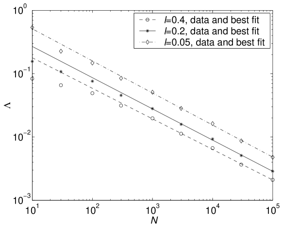
Figure 3.2: $\Lambda$ as a function of $N$ and $l$. The best fits are: for $l=0.4$, $\Lambda=(0.54\pm 0.07)N^{-0.483\pm 0.014}$; for $l=0.2$, $\Lambda=(0.83\pm 0.08)N^{-0.493\pm 0.09}$; for $l=0.05$, $\Lambda=(1.64\pm 0.16)N^{-0.507\pm 0.09}$.

Note also that the data points approach their asymptotic regimes very differently for different values of $l$: the bigger $l$ is, the lower the data start compared to their respective fits. This is explainable in view of the fact that smoother distributions usually vary over smaller ranges. For example, for $l=0.4$ the target distribution $P(x)$ usually takes values from $\sim 0.5$ to $\sim 2$. On the other hand, for not too large $N$ the estimates are also smooth and close to being uniform. Therefore, the KL divergence usually comes out small in this case. Thus the $l=0.4$ data starts so low not because we manage to learn the distribution extremely well for $N=10$, but because almost any guess is as good as any other at this level of detail.

3.4 Learning with ‘wrong’ priors

We stress first that there is no such thing as a wrong prior. If one admits the possibility of a prior being wrong, then that prior does not encode all of our a priori knowledge! It does make sense, however, to ask what happens if the distribution we are trying to learn is an extreme outlier in the prior ${\cal P}[\phi(x)]$. One way to generate such an example is to choose a typical function from a different prior ${\cal P}^{\prime}[\phi(x)]$, and this is what we mean by ‘learning with an incorrect prior.’ To study this we learn using $\eta=1$ and $l$, but we choose our target distributions from the prior Eq. (3.2) with different values of $\eta_{a}$ and $l_{a}$.

If the prior is wrong in the above sense, and the learning process is as usual, Eqs. (A.3, A.6–A.8), then we still expect the asymptotic behavior, Eq. (3.3), to hold. Indeed, once $\phi_{\rm cl}$ becomes close to $-\log P$, it takes the same time to discover that the distribution’s features at the current relevant scale $\xi(N)$ are as expected, too big, or almost absent. Thus only the prefactors of $\Lambda$ should change, and those must increase because there is an obvious advantage in having the right prior. We illustrate these points in Figs. (3.3, 3.4).

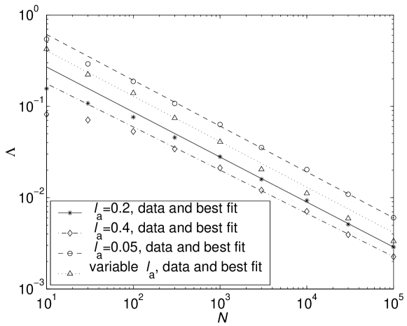
Figure 3.3: $\Lambda$ as a function of $N$ and $l_{a}$. Best fits are: for $l_{a}=0.4$, $\Lambda=(0.56\pm 0.08)N^{-0.477\pm 0.015}$; for $l_{a}=0.05$, $\Lambda=(1.90\pm 0.16)N^{-0.502\pm 0.008}$; for variable $l_{a}$, $\Lambda=(1.28\pm 0.13)N^{-0.498\pm 0.016}$. In all cases we learn with $l=0.2$.

Figure (3.3) shows the learning curve for distributions generated with the ‘actual’ smoothness scale $l_{a}=0.4,\,0.05$ and studied using the ‘learning’ smoothness scale $l=0.2$ (we show the case $l_{a}=l=0.2$ again as a reference). The $\Lambda\sim 1/\sqrt{N}$ behavior is seen unmistakably. The prefactors are a bit larger (unfortunately, insignificantly) than the corresponding ones from Fig. (3.2), so we may expect that the ‘right’ $l$, indeed, provides better learning (see Section 3.5 for a detailed discussion). Finally, the approach to the asymptotes again is different for the different examples considered, but it is still explainable by the argument we used for Fig. (3.2).

To generate outliers that are even more uncommon than the ones just discussed one may want to distort the $x$ axis (use different parameterization), and this results in a variable smoothness scale $l_{a}(x)$. As an example, Fig. (3.3) shows the learning curve for $l_{a}=0.2$ distributions that have been rescaled according to $x\to x-0.9\sin(2\pi x/L)$. For the rescaled variable, $l_{a}(x)$ varies from $0.02$ to $0.38$. Two separate straight line fits—through the first five (shown) and the last four points—are possible for this data. Each of the fits separately agrees with the prediction, but their prefactors are different. This is probably just a numerical artifact because $1000$ Fourier modes used here feel like much less in some places due to the rescaling, and this shows up at large enough $N$. Alternatively, this may be an indication that a detailed analysis of the reparameterization invariant formulation (Periwal 1997, 1998) is needed.

Finally, Fig. (3.4) illustrates learning when not only $l$, but also $\eta$ is ‘wrong’ in the sense defined above. We illustrate this for $\eta_{a}=2,\,0.8,\,0.6,\,0$ (remember that only $\eta_{a}>0.5$ removes UV divergences). Again, the inverse square root decay of $\Lambda$ should be observed, and this is evident for $\eta_{a}=2$. The $\eta_{a}=0.8,\,0.6,\,0$ cases are different: even for $N$ as high as $10^{5}$ the estimate of the distribution is far from the target, thus the asymptotic regime is not reached. This is a crucial observation for our subsequent analysis of the smoothness scale determination from the data (Section 3.5). Remarkably, $\Lambda$ (both averaged and in the single runs shown) is monotonic, so even in the cases of qualitatively less smooth distributions there is still no overfitting. On the other hand, $\Lambda$ is well above the asymptote for $\eta=2$ and small $N$, which means that initially too many details are expected and wrongfully introduced into the estimate, but then they are almost immediately ($N\sim 300$) eliminated by the data.

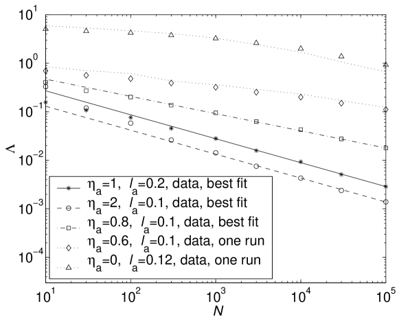
Figure 3.4: $\Lambda$ as a function of $N$, $\eta_{a}$ and $l_{a}$. Best fits: for $\eta_{a}=2$, $l_{a}=0.1$, $\Lambda=(0.40\pm 0.05)N^{-0.493\pm 0.013}$, for $\eta_{a}=0.8$, $l_{a}=0.1$, $\Lambda=(1.06\pm 0.08)N^{-0.355\pm 0.008}$. $l=0.2$ for all graphs, but the one with $\eta_{a}=0$, for which $l=0.1$.

3.5 Selecting the smoothness scale

Results presented in the last Figures already suggest that Occam factors should work in this infinite dimensional case, and that it indeed is possible to see this in numerical simulations. The competition between the data and the Occam factor is equivalent to minimizing the expression [cf. Eq. (A.6, A.7)]

$$H^{*}[\phi_{\rm cl};\{x_{\rm i}\};l]=\int dx\frac{l}{2}(\partial_{x}\phi_{\rm cl})^{2}+\sum_{j=1}^{N}\phi_{\rm cl}(x_{j})+\frac{1}{2}\sqrt{\frac{N}{ll_{0}}}\int dx\exp\left[-\phi_{\rm cl}(x)/2\right],$$ (3.9)

which makes the total probability of the data maximal, and thus the length needed to code it minimal. How does the smoothness scale $l^{*}$ that minimizes $H^{*}$ behave? The data term [second in Eq. (3.9)] on average is equal to $ND_{\rm KL}(P||Q_{\rm cl})$, and it can be small compared to the other terms for very regular $P(x)$. Then only the kinetic and the fluctuation terms matter, and $l^{*}\sim N^{1/3}$, as was obtained by Bialek, Callan, and Strong (1996). For less regular distributions $P(x)$ [cf. graphs for $\eta_{a}=0,0.6,0.8$ on Fig. (3.4)], this is not true. Indeed, for $\eta=1$, $Q_{\rm cl}(x)$ approximates large scale features of $P(x)$ very well, but details at scales smaller than $\sim\sqrt{l/NL}$ are not present in it. If $P(x)$ is taken from the prior, Eq. (3.2), characterized by some $\eta_{a}$ and $l_{a}$, then according to Eq. (3.8) the contribution of these details falls off with the wave number $k$ as $\sim(L/l_{a})^{\eta_{a}-1/2}k^{-\eta_{a}}$. Thus the expected data term is

$$ND_{\rm KL}(P||Q_{\rm cl})\sim N\int_{\sqrt{NL/l}}^{\infty}\;\left({L\over{l_{a}}}\right)^{2\eta_{a}-1}k^{-2\eta_{a}}=N\left({L\over{l_{a}}}\right)^{2\eta_{a}-1}\left({NL\over l}\right)^{-\eta_{a}+1/2},$$ (3.10)

and this is not necessarily small. For $\eta_{a}<1.5$ it actually dominates the kinetic term and competes with the Occam factor to establish the relevant smoothness scale. Summarizing,

$$l^{*} \sim N^{1/3},\,\,\,\,\,\eta_{a}\geq 1.5$$ (3.11)

$$l^{*} \sim N^{(\eta_{a}-1)/\eta_{a}},\,\,\,\,\,0.5<\eta_{a}<1.5\,.$$ (3.12)

There are two noteworthy things about Eq. (3.12). First, for $\eta_{a}=\eta=1$, $l^{*}$ stabilizes at some constant value, which we expect to be equal to $l_{a}$. Second, even if $\eta_{a}\neq\eta$, but $\eta_{a}<1.5$, then Eqs. (3.3, 3.12) ensure that $\Lambda\sim N^{1/2\eta_{a}-1}$, and this asymptotic behavior will be reached almost immediately, unlike in the $\eta_{a}=0,0.6$ examples from Fig. (3.4). This performance is, at most, a constant factor away from the limits set by heuristic calculations of predictive information, Eq. (2.99), with the ‘right’ priors $\eta_{a}=\eta\neq 1$—a remarkable result!

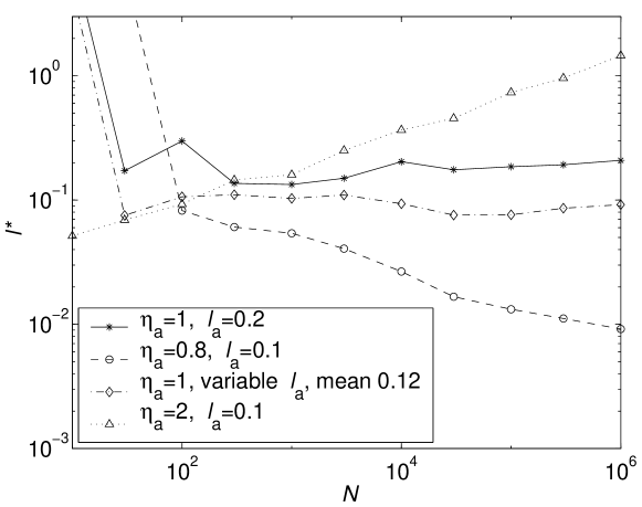
Figure 3.5: Smoothness scale selection by the data. The lines that go off the axis for small $N$ symbolize that $H^{*}$ monotonically decreases as $l\to\infty$.

We present simulations relevant to these predictions in Figs. (3.5, 3.6). Unlike in the previous Figures, these results are not averaged due to extreme computational costs, so all our further claims, which are inherently statistical, have to be taken cautiously. On the other hand, selecting $l^{*}$ and observing the effects associated with it in single runs has some practical advantages since then we are able to ensure the best possible learning for any given realization of the data, not just on average.

Figure (3.5) shows single learning runs for various $\eta_{a}$ and $l_{a}$. In addition, to keep the Figure readable, we do not show runs with $\eta_{a}=0.6,\,0.7,\,1.2,\,1.5,\,3$, and $\eta_{a}\to\infty$, which is a finitely parameterizable distribution. All of these display a good agreement with the predicted scalings, Eq. (3.11, 3.12).

Figure (3.6) shows the KL divergence between the target distribution and its classical estimate calculated at $l^{*}$; the average of this divergence over the samples and the prior is the learning curve. Again, the predictions are clearly fulfilled. Note that for all $\eta_{a}$ with exception of $\eta_{a}=\eta=1$ there is indeed a qualitative advantage in using the data induced smoothness scale. To illustrate this more clearly and ease the comparison we replotted some of the curves with adaptive $l$ side by side with their fixed $l$ analogues on Fig. (3.7).

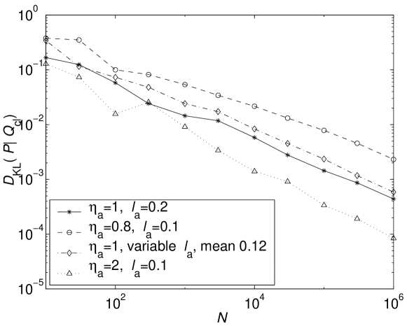
Figure 3.6: Learning with the data induced smoothness scale.

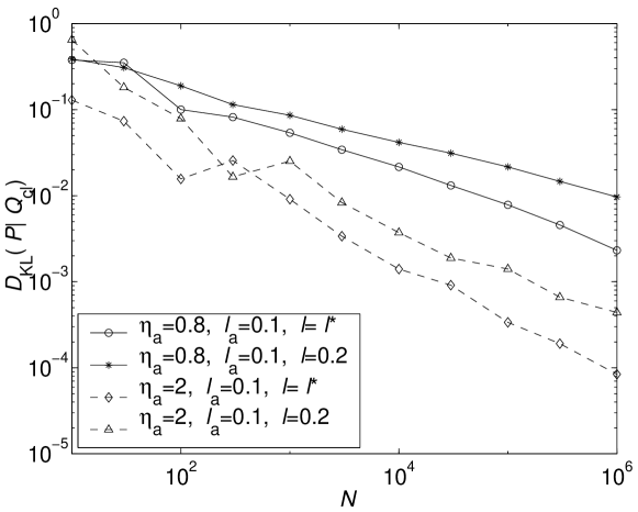
Figure 3.7: Comparison of learning speeds for the same data sets with different a priori assumptions. In all runs we learn using the model with $\eta=1$, and $l$ is either predefined, or set by the Occam factor.

3.6 Can the ‘wrong’ prior help?

The last four Figures have illustrated some aspects of learning with ‘wrong’ priors. However, more importantly, all of our results may be considered as belonging to the ‘wrong prior’ class. Indeed, the actual probability distributions we used were not nonparametric continuous functions with smoothness constraints, but were composed of $k_{c}$ Fourier modes and thus had exactly $2k_{c}$ parameters. Usually it would take well over $2k_{c}$ samples to even start to close down on the actual value of the parameters, and many more to get accurate results. However, using the wrong continuous parameterization [$\phi(x)$] we were able to obtain good fits for as low as $1000$ samples [cf. Figs. (3.1)] with the help of the prior Eq. (A.5). Moreover, learning happened continuously and monotonically without huge chaotic jumps of overfitting that necessarily accompany any brute force parameter estimation method at low $N$. So, for some cases, a seemingly more complex model is actually easier to learn!

We can summarize this by stating that, when data are scarce and the parameters are abundant, one gains even by using the regularizing powers of wrong priors. The priors select some large scale features that are the most important to learn first and fill in the details as more data become available. If the global features are dominant (arguably, this is generic), one actually wins in the learning speed [cf. Figs. (3.2, 3.3, 3.6)]. If, however, small scale details are as important, then one is at least guaranteed to avoid overfitting [cf. Fig. (3.4)].

Thus we can argue that our numerical experiments support the Occam–like claim we made in Section 2.6: if two models provide equally good fits to data, the simpler one should always be used. In particular, using Eq. (2.102) we see that for our simulations, the nonparametric QFT model is simpler (as characterized by the predictive information) than a finite dimensional one for $N<N_{c}\sim(k_{c}\log k_{c})^{2}$. We operate in this regime in all of our simulations, and so we must learn faster and with less overfitting if we use the wrong parameterization. Note, that these results are very much in the spirit of our whole program: not only is the value of $l^{*}$ selected that simplifies the description of the data, but the continuous parameterization itself serves the same purpose. This is an unexpectedly neat generalization of the MDL (Rissanen 1989) principle to nonparametric cases.

3.7 Discussion

The field theoretic approach to density estimation in principle not only regularizes the learning process but also allows the self–consistent selection of smoothness criteria through an infinite dimensional version of the Occam factors. We have shown numerically that this works, even more clearly than was conjectured. For $\eta_{a}<1.5$, $Q_{\rm est}$ and the learning curve $\Lambda$ truly become properties of the data and not of the Bayesian prior used for learning: one can set a learning machine to work at $\eta=1$ and be sure that this does not bias the estimates in any excessive way. If we can extend these results to include $\eta_{a}>1.5$ and combine this work with the reparameterization invariant formulation of Periwal (1997, 1998), this should give a complete theory of Bayesian learning for one dimensional distributions, and this theory has no arbitrary parameters. In addition, if this theory properly treats the limit $\eta_{a}\to\infty$, we should be able to see how the well–studied finite dimensional Occam razors and the MDL principle arise from a more general nonparametric formulation.

These results also have some biological implications. First of all, it may be that this smoothness scale adaptation mechanism is partly responsible for a commonly known effect: children learn faster than adults. More seriously, and more closely connected to the models discussed here is the learning and development of smooth ‘maps’ in the nervous system (see, for example, Knudsen et al. 1987). These maps become much less susceptible to the sensory inputs as time passes, and this may be interpreted in terms of stiffening of the smoothness constraint. Indeed, starting from scratch, it is very easy to drift the smoothness scale to such large values that susceptibility of the learning machine (in other words, an animal) to the new data will be extremely small.

Second, if our conclusions are correct, then a learning machine that is programmed to solve problems at $\eta=1$ can easily solve more complex problems with any $\eta_{a}$, $1.5>\eta_{a}>0.5$, by performing a simple averaging over the smoothness scales. At worst, this procedure may lead to a constant multiplicative drop in performance. By analogy, we may expect that, once an animal is able to treat a problem that falls in any power–law class with respect to the predictive information, then it is able to treat any problem that provides more predictive information with only a multiplicative overhead. Since, as we have already discussed (Hilberg 1990, Ebeling and Pöschel 1994, Pöschel, Ebeling, and Rosé 1995), humans can solve power–law problems, it is encouraging to know that there is no learning task in this world that is, in principle, too difficult for us (our lifetime is the only limiting factor). More seriously, if it is, indeed, possible to construct a complete theory of one (and, possibly, higher) dimensional learning, where both the smoothness scale and the exponent can be self–consistently determined, then the questions we asked in Section 2.6 (like “what models do humans use for learning?”) may lose their meaning—any model is almost as good as any other, and it is very difficult to look for possible multiplicative differences between them. Surprisingly, these questions are meaningful if such a theory cannot be constructed. In this case, as we saw in Eqs. (3.11, 3.12) and on Figs. (3.5, 3.6), a complex learning machine cannot effectively adapt to simple tasks. This again accords with our subjective experience that it is sometime very hard to find a simple solution when expecting a complex one. It should be possible to devise an experiment that would quantify this failure to solve simple problems in complex contexts.

Chapter 4 Learning discrete variables:
Information–theoretic regularization

4.1 The general paradigm

In Chapters 2 and 3 of this work we discussed what we consider to be some of the most interesting problems in modern statistics and learning theory. We defined predictive information and complexity, studied the learning of nonparametric distributions, and showed an example of how Occam factors generalized to infinite dimensional problems. There is one tantalizing question that followed us through this whole discussion: many problems require a prior to regularize learning, but then how can one make sure that the estimates and the conclusions are inferred from the data, rather then being imposed by some a priori knowledge that the data do not support? The results in the infinite dimensional generalization of the Occam factors seemed especially interesting in this respect—estimates can become almost insensitive even to the qualitative choice of prior, at least in a broad range. This conclusion, together with Periwal’s (1997, 1998) work, are the only results known to us that aim towards constructing a reparameterization and prior invariant (or, better yet, ignorant) theory of nonparametric Bayesian inference.

Even though we have concentrated on nonparametric problems, similar difficulties also exist in seemingly simpler, parametric cases. The choice of the prior for finite parameter learning scenarios is still a hot topic, and various alternatives are proposed that make some universal theoretical sense within the framework of information theory, MDL theory, etc. Examples include universal priors (Rissanen 1983, Lee and Vitányi 1993) or Jeffreys’ priors (Clarke and Barron 1994, Balasubramanian 1997).

We think, however, that the prior really should embody a priori knowledge, and thus we cannot agree with the use of universal, globally definable choices. On the other hand, there is an obvious appeal for approaches based on more general theoretical principles. For example, the problems of nonuniform convergence of the estimate to the target, Eq. (A.11), and of the infrared divergence of predictive information, Eq. (2.97), are easily resolved if one turns to reparameterization invariant priors (Periwal 1997, 1998). These have a clear theoretical edge over non–invariant ones since they estimate a true density, that is, a function that transforms like a density under reparameterizations of the independent variable.

As we tried to emphasize in this work, learning is information accrual, and, therefore, it is a part of Shannon’s information theory. Thus a general theoretical principle can be to construct priors solely from information–theoretic quantities like entropy (or self–information), Kullback–Leibler divergence (or relative information), various mutual informations, etc., and with no other constraints. In addition, since information–related quantities are formed from log–probabilities it makes sense to include them exponentially into the priors, which are, after all, also probabilities. In Sections 4.3 and 4.4 we will present a simple example that illustrates the use of this general principle—regularization with information–theoretic quantities—and show that it is possible and advantageous to learn with such priors.

4.2 Discrete variables: a need for special attention

When learning probability densities of continuous variables, except for the very simple cases $N>>d_{\rm VC}$, priors are used to balance the quality of fits to the data against the complexity of solutions (cf. Section 2.4.5 and Chapter 3); this smoothing of data prevents overfitting. It is easy to construct smoothing priors for continuous variables: continuity implies a metric, so locality is defined, and then one just needs to punish distributions that exhibit large variations over small distances. Such a ‘smoothness’ prior will work as a regularizer.

The case when a variable is discrete, and the (discrete) metric is impossible to define, presents a problem. Usually this case is not considered interesting, because the law of large numbers guarantees that, at large $N$, the frequencies of events estimate probabilities well. However, if the number of examples $N$ is smaller or comparable to the number of possible outcomes $K$, then statistical fluctuations are large. This situation is not as uncommon as one might hope. For example, it is possible that syntactic structures in a language can be inferred from statistical arguments alone (see, for example, Pereira et al. 1993, Manning and Schütze 1999). Estimating probabilities of occurrence of a few thousand common words is rather easy. It is even feasible to construct conditional distributions of nouns given verbs (Pereira et al. 1993). However, it is totally unrealistic to expect to build an accurate probability distribution of whole sentences from the raw data without some a priori knowledge.

Similar problems appear in molecular biology. For example, gene expression is governed by promoter regions in DNA molecules. These regions are usually thought to be constructed from two five base pair long blocks (there are $4^{5}$ possible different realizations of these) that appear anywhere inside ‘junk’ genetic material, which is about a hundred bases in length. If one tries to find the meaningful $5+5$ structures by statistical methods (see, for example, van Helden et al. 1998), then a probability distribution over $4^{5}*4^{5}\sim 10^{6}$ possibilities must be constructed. Many experiments are done on yeast, and their genome is only a few millions of base pairs long. So getting a full statistics is, at best, problematic. Even worse, if one tries to look for a possibility of promoters of a different length, then the problem becomes totally hopeless.

To solve these and similar problems, one needs smoothing priors that regularize fluctuations. However, now there is no notion of locality to create them. It is not at all evident how to impose smoothness conditions, or whether these conditions will speed up learning in any way. It is clear though that any smoothing must be global—we cannot talk about local changes, but global variability is well defined. Recall that variability can be measured non–metrically by entropies, and these have a very special meaning in information theory—they are the unique measure of information (Shannon 1948). Therefore, learning a discrete variable may turn out to be an excellent example of the general paradigm introduced above.

In the next Sections we present a toy model for learning a discrete variable and show that it is possible to regularize and speed up such learning with the help of information–theoretic priors. In general, discrete calculus is much less developed than its continuous analogue (precisely for the reason that the notion of locality is absent), so analytical results can usually be achieved only for very simple problems, and our example is like that. Nonetheless, this case is of interest as it solves some real world problems and, more importantly, because it develops techniques that later will be used in more complicated tasks; the work on those is already in progress.

4.3 Toy model: theory

Consider the following ‘real world’ problem. A US Census Bureau needs a preliminary report on statistics of people in Trenton, NJ based on the Census–2000 data. Unfortunately, only a few thousand households have filled in their Census cards, and this is clearly not enough to sample adequately many classes $x,\,x=1\cdots K$ (we also call them possible outcomes or bins) into which the people are classified (ethnicity, marital status, educational level, size of the household, etc.) Suppose now that Newark, NJ, perceived to have a similar population statistics, has been quick to organize door–to–door counting of people, so that a good sampling of Newark’s population, $Q^{*}(x)$, is available. Can the Census Bureau statisticians use these data to answer their questions about the Trenton people? An obvious solution would be to take a weighted average of the (undersampled) Trenton counts and the (well sampled) Newark probabilities. But how should the weights be set in order to ensure that the Trenton estimate is just smoothed and not unfairly biased by the Newark data?

We can offer a solution to the problem by choosing an a prior probability density for $Q(x)$, the Trenton distribution, that is biased towards the reference Newark distribution $Q^{*}(x)$. This may be done in the following form

$${\cal P}[Q(x),\lambda]=\frac{1}{{\cal Z}_{Q}(\lambda)}\exp\left[-\lambda D(Q^{*}||Q)\right]\,\delta\left(\sum_{x=1}^{K}Q(x)-1\right)\,{\cal P}(\lambda),$$ (4.1)

where ${\cal P}(\lambda)$ is some a priori normalized density for the inverse temperature–like parameter $\lambda$, ${\cal Z}_{Q}(\lambda)\equiv\int[dQ(x)]{\cal P}[Q(x)||\lambda]$ is the normalization of the a priori distribution of $Q(x)$ conditional on $\lambda$, and $D$ is some measure of distance between the two distributions, $Q^{*}$ and $Q$. If we want to stick to our paradigm of using information–theoretic quantities only, then we do not have much freedom in selecting $D$ since the natural distance between any two distributions in information theory is the familiar Kullback-Leibler divergence,

$$D(Q^{*}||Q)\equiv D_{\rm KL}(Q^{*}||Q)=\sum_{x=1}^{K}Q^{*}(x)\log\frac{Q^{*}(x)}{Q(x)}.$$ (4.2)

In the language of coding theory, this choice of $D$ means that we optimize our coding strategies for $Q$, but we want $Q$’s such that the data coming from the reference distribution can be coded compactly also. We could have chosen to measure distances in the opposite direction and switch arguments in the KL divergence. Then the best coding for $Q^{*}$ is fixed, and we look for $Q$ that is still coded well. We chose Eq. (4.2) over the other choice because this allows an exact solution.

Now, similarly to Bialek et al. (1996, see also Appendix A.1), we apply the Bayes formula to get the probability density for $Q(x)$ and $\lambda$ given the data $\{x_{\rm i}\}$

$$P[Q(x),\lambda|\{x_{\rm i}\}] = \frac{P[\{x_{\rm i}\}|Q(x),\lambda]\,{\cal P}[Q(x),\lambda]}{P(\{x_{\rm i}\})}$$ (4.3)

$$= \frac{{\cal P}[Q(x),\lambda]\prod_{i=1}^{N}Q(x_{\rm i})}{\int[dQ(x)]d\lambda{\cal P}[Q(x),\lambda]\prod_{i=1}^{N}Q(x_{\rm i})}\,.$$

The least square estimator of $Q(x)$ is then, as usual,

$$Q_{\rm est}(x|\{x_{\rm i}\}) = \int d\lambda[dQ(x)]\;Q(x)\,P[Q(x),\lambda|\{x_{\rm i}\}]$$ (4.4)

$$= \frac{\langle Q(x)Q(x_{1})Q(x_{2})\cdots Q(x_{N})\rangle^{(Q,\lambda)}}{\langle Q(x_{1})Q(x_{2})\cdots Q(x_{N})\rangle^{(Q,\lambda)}}\,,$$

where $\langle\cdots\rangle^{(Q,\lambda)}$ stands for averaging over $Q$ and $\lambda$ with respect to the prior; similarly, $\langle\cdots\rangle^{(Q)}$ means averaging only over ${\cal P}[Q|\lambda]$.

If $\lambda$ was fixed, then the averaging in Eq. (4.4) would have one integral less—a simpler problem. However, varying it may allow the Occam factor that arises from volumes in the $Q$-space to find some $\lambda^{*}$ that creates the shortest (thus the most probable) description of the data (cf. Section 3.5). By achieving the optimal balance between the ‘goodness of fit’ and closeness to the reference, this may resolve the problem of a possible erroneous bias towards $Q^{*}$.

As mentioned above, the solution of this model is rather simple. We write $n(x)$ for the data count in the bin $x$, $\sum_{x}n(x)=N$. Then, leaving aside the $\lambda$ integral for a while, we have (see Appendix A.2):

$$\langle Q(x_{1})\cdots Q(x_{N})\rangle^{(Q)} = \int[dQ]\frac{{\rm e}^{-\lambda D_{\rm KL}(Q^{*}||Q)}}{{\cal Z}_{Q}(\lambda)}\delta(\sum_{x}Q(x)-1)\prod_{x}Q(x)^{n(x)}$$ (4.5)

$$= \frac{{\rm e}^{S[Q^{*}]}}{{\cal Z}_{Q}(\lambda)}\int[dQ]\delta(\sum_{x}Q(x)-1)\prod_{x}Q(x)^{n(x)+\lambda Q^{*}(x)}$$ (4.6)

$$= \frac{{\rm e}^{S[Q^{*}]}}{{\cal Z}_{Q}(\lambda)}\;\frac{\prod_{x=1}^{K}\Gamma\Big{(}n(x)+\lambda Q^{*}(x)+1\Big{)}}{\Gamma(\lambda+N+K)},$$ (4.7)

where $S[Q^{*}]$ is just the entropy of the reference distribution. ${\cal Z}_{Q}(\lambda)$ is given by the same integral, Eq. (4.5, 4.7), but with $n(x)=N=0$. Therefore, if we now integrate over $\lambda$ using the steepest descent technique, then the most probable value of the inverse temperature is determined by

$$\sum_{j=1}^{N}\frac{1}{\lambda^{*}+K+j-1}-\sum_{x=1}^{K}\sum_{j=1}^{n(x)}\frac{Q^{*}(x)}{\lambda^{*}Q*(x)+j}=0.$$ (4.8)

Numerically (cf. Section 4.4) this equation has one nontrivial solution for large $N$, so that the Occam factor seems to work again. Unfortunately, however, we were unable to obtain satisfying analytical results with exception of some trivial asymptotic limits. If, on the other hand, we keep $\lambda$ fixed, then [see Eq. (4.4)]

$$Q_{\rm est}(x|\{x_{\rm i}\};\lambda)=\frac{n(x)+\lambda Q^{*}(x)+1}{N+\lambda+K}$$ (4.9)

The simplicity of this result is intriguing. Our initial suggestion to average the actual undersampled data with the well sampled smoothing distribution turns out to have deep roots in Bayesian inference with the prior Eq. (4.1)!

Note the presence of ‘$+1$’ in Eqs. (4.7, 4.9). Due to this term the estimated distribution is a smoothed version of the counts $n(x)$ even if $\lambda\to 0$. In this theory, no bin has an estimated probability of zero, so that $D_{\rm KL}(Q^{*}||Q)$ always is well defined, and observing the next sample in any bin never is a completely unexpected event. This summand, which has so many desirable consequences, appears because we define the prior, Eq. (4.1), on the space of $Q$’s. Changing the variables from probabilities to likelihoods, $-\phi(x)=\log Q(x)$, creates a Jacobian which effectively adds one count in every bin. Maximal likelihood estimation of parameters does not have this feature, and this is yet another argument in favor of the Bayesian formulation.

Even though this toy model has an exact solution, it still is instructive to perform a saddle point (large $N$) analysis in the hope that some useful knowledge reusable in more complex settings will be gained. With the usual change of variables,

$$Q(x)={\rm e}^{-\phi(x)},\,\,\,\,\,Q^{*}(x)={\rm e}^{-\phi^{*}(x)},$$ (4.10)

leaving the $\lambda$ integral aside again, and replacing the $\delta$-function by its Fourier representation, we get the following expression for the correlation functions:

$$\langle Q(x_{1})\cdots Q(x_{N})\rangle^{(Q)} = \int\frac{[d\phi(x)]}{{\cal Z}_{Q}(\lambda)}\frac{d\mu}{2\pi}{\rm e}^{-H[\phi(x),i\mu,\lambda,\phi^{*}(x)]-\sum_{x}[n(x)+1]\phi(x)},$$ (4.11)

$$H[\phi(x),i\mu,\lambda,\phi^{*}(x)] = \lambda\sum_{x}Q^{*}(x)[\phi(x)-\phi^{*}(x)]+i\mu(\sum_{x}{\rm e}^{-\phi(x)}-1).$$ (4.12)

Calculating up to one–loop corrections using the steepest descent techniques, this Hamiltonian results in

$$\langle Q(x_{1})\cdots Q(x_{N})\rangle^{(Q)} = {\rm e}^{-H_{\rm eff}[\phi_{\rm cl}(x),\lambda,\phi^{*}(x)]-\sum_{x}[n(x)+1]\phi_{\rm cl}(x)},$$ (4.13)

$$H_{\rm eff}[\phi_{\rm cl}(x),\lambda,\phi^{*}(x)] = H[\phi_{\rm cl}(x),i\mu=N+\lambda+K,\lambda,\phi^{*}(x)]$$ (4.14)

$$+ \frac{K}{2}\log\left(1+\frac{N}{\lambda}\right)+\frac{1}{2}\sum_{x}(\phi^{*}(x)-\phi_{\rm cl}(x)),$$

$$Q_{\rm cl}(x) \equiv {\rm e}^{-\phi^{\rm cl}(x)}=\frac{n(x)+\lambda Q^{*}(x)+1}{N+\lambda+K}$$ (4.15)

Again, just like in Eqs. (3.1, A.7), the fluctuation determinant [the last two terms in Eq. (4.14)] has a different $\lambda$ dependence than the data and the prior terms. This suggests, even more clearly than the exact result Eq. (4.7), that competition between them will select a nontrivial most probable value of $\lambda^{*}$.

Note that $Q_{\rm est}$, Eq. (4.9), is equal to $Q_{\rm cl}$. A priori one should not expect them to be similar even for large $N$. Indeed, the matrix of second derivatives in the saddle point calculation has eigenvalues $\sim n(x)$, and these are small for bins with small counts. So, in principle, one could expect large discrepancies between the exact and the classical solutions. The fact that they are the same inspires a hope that the saddle point analysis may remain useful for other, more complex, problems.

Finally, we want to illustrate yet another important aspect of this toy model. What is the predictive information for this system? In general, it is difficult to calculate, so we consider two very simple limits: $\lambda\ll N,\,K\ll N$, and $1\ll N\ll\lambda,K\ll\lambda$. The first case closely parallels calculations of Section 2.4.2 and yields

$$S_{1}(N)\approx\frac{K}{2}\log N.$$ (4.16)

In the second case, somewhat lengthy calculations lead to

$$S(N)=NS[Q^{*}]+S_{1}(N),\,\,\,\,\,\,\,\lim_{N\to\infty,N/\lambda\to 0}S_{1}\approx{\rm 0},$$ (4.17)

where $S[Q^{*}]$ is again the entropy of the reference distribution. These results are expected: for small $\lambda$ and large $N$ this problem is just learning a $K$–parameter distribution, so Eq. (2.50) should hold. On the other hand, for extremely large $\lambda$, the estimate converges to the reference distribution regardless of the data, so the problem is effectively zero dimensional.

If we do estimates at some large, but fixed, $\lambda$, then we should see a crossover from the zero to the $K$ parameter regime. For generic distributions the crossover will be smooth, since each bin starts to add its $(1/2)\log N$ to the predictive information independently when the estimate for that bin switches from the reference value to the count, i. e., when $n(x)>\lambda Q^{*}(x)$ [cf. Eq. (4.9)]. A smooth crossover from zero to the logarithm is possible only through a faster than logarithmic growth for some range of $N$. Indeed, from the discussion in Section 2.4.6, we know that continuous addition of extra degrees of freedom is a sign of the power–law growth of predictive information. It is remarkable that a discrete system as simple as this toy model can exhibit such a rich behavior that, so far, has been associated with only very complex nonparametric models; we will see a numerical demonstration of this in the next section.

4.4 Toy model: numerical analysis

If we want to be able to observe all of the features described in the previous section, then $K$, the number of bins, should be large enough to allow for a prominent prior–dominated (scarce data) region, but it also should be small enough so that we can generate enough samples and observe a cross–over to the data–driven regime in all bins. The choice of $K=75,100,125$ reasonably satisfies both conditions and will be used in all of our simulations.

The next important question is the generation of random distributions from the prior, Eq. (4.1). Due to the $\delta$-function normalization constraint this is a complicated task. However, in the limit of large $\lambda$, $D_{\rm KL}[Q^{*}||Q]$ typically is small and can be approximated by the $\chi^{2}$ distance

$$\lim_{D_{\rm KL}\to 0}D_{\rm KL}[Q^{*}(x)||Q(x)]={1\over 2}\sum_{x=1}^{K}\frac{[Q(x)-Q^{*}(x)]^{2}}{Q^{*}(x)}.$$ (4.18)

Then the prior, Eq. (4.1), becomes a multi–variable normal density, and generation of random distributions is easy .

The choice of $\lambda$ is motivated by the same arguments as the choice of $K$. The asymptotic regime is reached for $\lambda K>N$, while simulations are time limited by $N\sim 10^{5}$. Therefore, we must use $\lambda$ of up to about $1000$. On the other hand we want to see as much of the prior–enforced learning as possible, so we choose to work close to this limit: $\lambda=300,500,1000$. One may be concerned that these large values will produce random distributions that are almost identical to the reference, which would make some of our results less interesting. Fig. (4.1) shows that these fears are misplaced. The reference and the random distributions are similar (as we want them to be), but not excessively so.

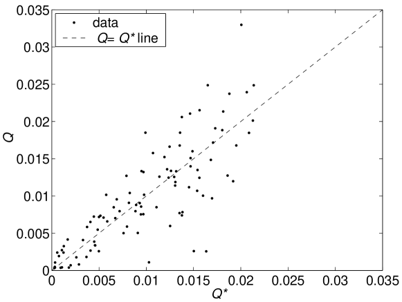
Figure 4.1: Comparison between the reference distribution and a typical random one generated with $\lambda=500$, and $K=100$. Each point corresponds to the values $\Big{(}Q^{*}(x),Q(x)\Big{)}$ in one of the bins $x$.

4.4.1 Learning with the correct prior

Fig. (4.2) shows the $N$ dependence of the universal learning curve $\Lambda$ [averaged KL divergence, Eqs. (2.13, 3.3)], for various combinations of $\lambda$ and $K$. All of the behavior predicted in Section 4.3 is observed clearly. The learning curves start out flat (predictive information and the effective number of parameters are zero) and soon enter a continuous series of transitions that add more and more degrees of freedom. Finally the behavior enforced by Eq. (2.62),

$$\Lambda(N)=\frac{K}{2N},$$ (4.19)

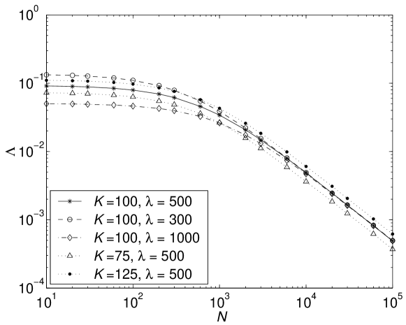
Figure 4.2: $\Lambda$ as a function of $\lambda$, $K$, and $N$ for $\lambda=\lambda_{a}$.

is reached. Notice that, in agreement with the claim that the number of active parameters depends on the comparison between the counts and the value of $\lambda$, the asymptotic regime is reached at earlier $N$ for smaller values of the parameter. The agreement with this asymptotic behavior is so remarkably good that we chose not to quote any fits: all of them are within the expected errors.

In the pre–asymptotic regime, learning curves with larger $\lambda$ start lower since there the random distributions are very close to the reference and are estimated much better by it. Similarly, curves with smaller $K$ also start lower because now there are fewer degrees of freedom and, therefore, fewer ways to get a larger KL divergence.

4.4.2 Learning with ‘wrong’ priors

As we did for nonparametric distributions in Section 3.4, we now want to investigate the performance of the learning algorithm on atypical data sequences. That is, as before, we will differentiate two sets of parameters: $\lambda$ and $Q^{*}$, which encode the expectations of the learning machine, and $\lambda_{a}$ and $Q^{*}_{a}$, which together with Eq. (4.1) describe the ensemble of atypical target distributions. Simulations related to this question are summarized in Fig. (4.3). Here we have shown learning with different combinations of $\lambda\neq\lambda_{a}$, and the case $\lambda=\lambda_{a}=500,Q^{*}=Q^{*}_{a}$ is plotted as a reference. Comparing the curves with the corresponding ones from the previous Figure, we clearly see that, even though learning with an ‘incorrect’ prior is possible, there are discrepancies: convergence to the asymptotic limit is different, and the curves start slightly higher then their ‘correct’ counterparts.

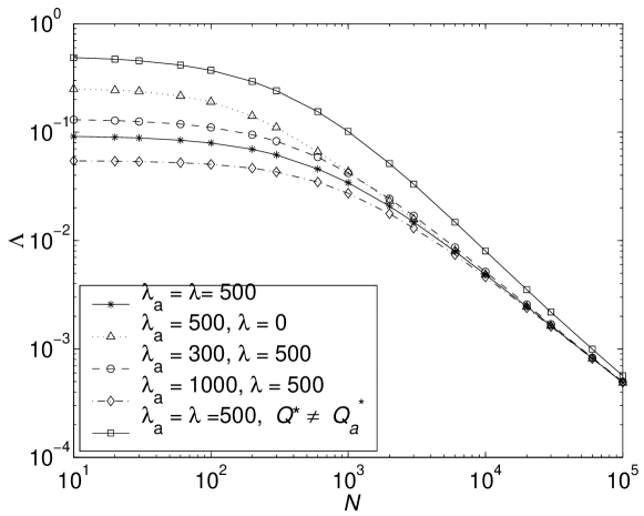
Figure 4.3: $\Lambda$ as a function of $\lambda$, $\lambda_{a}$, $Q^{*}_{a}$ and $N$. For all curves $K=100$.

Another interesting example shown is when $\lambda$ is ‘correct’, but the reference distribution itself is totally wrong. We see that this type of mistake is much more costly: even for $N$ as large as $10^{5}$ the influence of the wrong reference distribution is still strong enough to compromise fast learning.

Note the curve with $\lambda_{a}=500$, $\lambda=0$. This is a case of ‘trivial’ learning, when the only regularization is due to the Jacobian of the $Q\to\phi$ transformation [the ‘$+1$’ term in Eq. (4.9)]. If not for it, the estimate would be extremely overfitted and would have zeros, and the $\Lambda$ would explode. On the other hand, with the ’$+1$’ correction, $\Lambda$ starts out from a constant value, which is the KL divergence between the target and the uniform distribution.

4.4.3 Selecting $\lambda$ with the help of the data

Having shown how the learning machine performs on expected and unexpected data samples, we are now in a position to ask if the Occam factors can select the right regularization parameter $\lambda$ as in the case of finite dimensional models (MacKay 1992, Balasubramanian 1997) and nonparametric models (Bialek, Callan, and Strong 1996, and Section 3.5 of the present work). This question has an affirmative answer, and Fig. (4.5) shows $\lambda^{*}$, the value of $\lambda$ that maximizes the correlation function Eq. (4.7) and minimizes the exponent in Eq. (4.13).

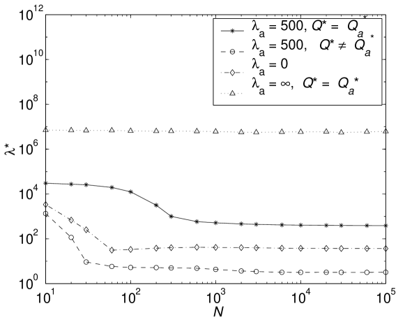
Figure 4.4: $\lambda^{*}$ for various ensembles of target distributions.

We show the results averaged over many runs, even though this form of presentation is questionable because $\lambda^{*}$ fluctuates a lot in different trials. These fluctuations explain the kinks on the three lower curves. For $N$ to the left of the kinks, there are many realizations of the data, for which there is no best value for $\lambda$, and the correlation functions are maximized at $\lambda^{*}\to\infty$. The kinks appear due to the numerically imposed finite cutoff on possible values of the parameter. Apart than this, the rest of the learning curves’ behavior is as hoped. For ensembles generated at $\lambda_{a}=500$ and studied at $Q^{*}=Q^{*}_{a}$, $\lambda^{*}$ turns out to be very close to 500. If $Q^{*}\neq Q^{*}_{a}$, $\lambda^{*}$ drifts to smaller values, letting the data, not the reference, control the estimate. The same happens for $\lambda_{a}=0$ for any $Q^{*}$ since at this value of the parameter the target is, again, far from the reference.

Finally, we examine the case where the ensemble of the distributions is qualitatively closer to the reference than the prior, Eq. (4.1), allows (this corresponds to $\eta\neq\eta_{a}$ for nonparametric learning). This can be achieved by having a higher power of the KL divergence in the exponent of the prior, but such a choice is very difficult for numerical simulations. So we take an easier, but less illustrative example of $\lambda_{a}=\infty$; that is, the target distribution is exactly equal to the reference. Here, not surprisingly, $\lambda^{*}$ quickly becomes very large. Again, it often exceeds the numerical cutoff, so the average line shown should not be taken to literally.

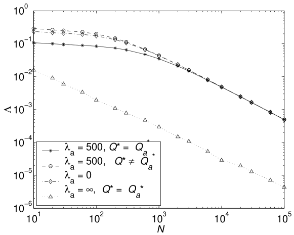
Figure 4.5: Learning with an adaptive $\lambda^{*}$.

Finishing up this section, in Fig. (4.4) we show the learning curves calculated at $\lambda=\lambda^{*}$ for all the cases considered above. Comparing to the corresponding learning curves in Fig. (4.3), we deduce that learning with an adaptive $\lambda$ is much faster than with a fixed wrong one, and the example with $\lambda_{a}=\infty$ is particularly demonstrative . The only learning curve which starts off slightly worse than its fixed $\lambda$ analogue is that for $\lambda_{a}=500,\,Q^{*}=Q^{*}_{a}$. Even though it improves very quickly, this once again proves the common knowledge that for small sample sizes nothing beats learning with the ‘correct’ prior.

4.5 Further work

The toy example we have investigated resolves the questions it was meant to answer. Yet it is just a toy example, and most of its value lies in the extension to more difficult problems.

The most straightforward, but very interesting development is one that has been already mentioned in passing. Reversing the direction of the KL divergence in Eq. (4.1) and choosing a uniform reference distribution $Q^{*}$, we obtain a prior that favors distributions with larger entropies, i. e., the flattest and the most regular distributions. Finding the least variable distribution compatible with the data is certainly in the spirit of our work and deserves an investigation.

This idea may be made more sophisticated when the independent variable is a vector, $\vec{x}=\{x,y\}$. If the distribution $Q({\vec{x}})$ is expected to be smooth, but the cardinalities of $x$ and $y$ ($K_{x}$ and $K_{y}$ respectively) are large, then only the marginal distributions $Q(x)=\sum_{y}Q(x,y)$ and $Q(y)=\sum_{x}Q(x,y)$ are sampled well for $K_{x}$ and $K_{y}\ll N\sim K_{x}K_{y}$. To smooth the data we might want to weight the a priori probability of $Q(x,y)$ by the entropy $S[Q(x,y)]$. However, this choice, though valid, is not the best. Indeed, the entropy can be small because the marginals are very narrow. But in the limit we are interested in, the marginals are well defined by the data and do not require separate smoothing. So it is not the entropy of a distribution, but its value with respect to the entropy of the marginals that should enter a regularizing prior. This is the mutual information $I(x,y)$ between $x$ and $y$, and it is, once again, a meaningful information–theoretic quantity.

A more ambitious but very appealing direction is to combine these methods with the relevant information extraction ideas of Tishby et al. (1999) and Bialek and Tishby (in preparation), discussed briefly in Section 2.6. Recall, that these authors proposed to compress (that is, to smooth) the variable $x$ into $\hat{x}$ so that the mutual information $I(\hat{x},y)$ remains as close to $I(x,y)$, as possible. There is a one parameter family of solutions to the problem, and this parameter measures the relative importance of compression (smoothing) and preservation of the information (fit to the data). In many practical applications, choosing the right value of this parameter is a problem. We can view the result of Tishby et al. as a classical solution to a problem with some (yet to be defined) prior. One can realistically expect that the value of the parameter will, once again, be set by the Occam factor.

If this theory succeeds, we can use these results to further advance the theory of learning a nonparametric variable. Derivatives of densities do not have any special meaning in the framework of information theory. Using them, as in Eq. (A.5) or its reparameterization invariant version (Periwal 1997, 1998), is thus not a preferred regularization. Building priors that include terms with derivatives of many different orders and fixing coefficients of the terms by requiring that the estimate does not depend on the UV details of the data (rounding or truncation) may work and have a meaning in QFT, but this is an approach alien to information theory. Similarly, preferring distributions that are close to their filtered version and averaging over the filters afterwards has the same problem. What we mean by smoothness in any formulation, including nonparametric continuous ones, is that the independent, possibly continuous, variable $x$ can be successfully coded in some $\hat{x}$ of finite and small cardinality such that this compacted version explains the data almost as well as the original one. For example, in the finite parameter case, $\hat{x}={\mbox{\boldmath$\alpha$}}$. Developing a theory for smoothing through compression would be a great achievement in itself, and within this formalism we get the added advantage that the right balance between the goodness of fit and the compression will again be determined by the Occam factor.

This is obviously only a start to an extensive program of generalizations, and we hope make a significant progress along these lines in the near future.

Chapter 5 Conclusion: what have we achieved?

Let us summarize our achievements and compare them to the promises we made and the desires we expressed in the beginning of this work. As promised, we built a uniform and universally valid approach to learning by using information theory and treating learning as an ability to predict. For this we defined a new quantity, the predictive information, and the study of it revealed that it not only measures the information relevant to prediction of a time series, but also defines uniquely the complexity of the process that generated the series. Statistical mechanics gave an insight on how learning is always annealing in the model space, and then we could illuminate numerous connections to statistical learning and coding theories and catch some omissions in those. Summarizing, we indeed delivered on the promise of a coherent re–treatment of the old knowledge.

Then we went further and showed that conventional finite parameter models are not the only possible scenario. We investigated nonparametric and (undersampled) discrete learning to show that the capacity control mechanisms work much better then one might have thought. We showed that the ’information theory only’ approach to learning can be made self consistent and does not need any supplemental help to survive. All of these efforts constitute an attempt to build up some new flesh around the core of ideas that are the focal point of our attention. This flesh may seem too thin, and it certainly is—a lot more has to be done before one can finally say: “The End!” However, one has to start somewhere, and we did.

Appendix A Appendix

A.1 Summary of nonparametric learning

The main problem of statistics—inferring distributions from a finite data set— has a wide variety of possible practical applications. Usually, based on some a priori considerations, an observer has some finite-dimensional model for the distribution being studied. Then the problem reduces to an estimation of a finite number of parameters from a large data set, and this is relatively well-studied (see, for example, Vapnik 1998, Balasubramanian 1997, and Sections 2.4.1–2.4.5 of the current work). Unfortunately, reducing the problem to a finite number of parameters heavily biases the outcome of statistical inference: the true distribution may not even be in the chosen family. Thus lately it has become popular to look for nonparametric solutions to the problem of learning distributions (recent reviews are Dey et al. 1998 and Lemm 1999). As discussed in Section 2.4.5, nonparametric estimations necessarily are prior dependent, i. e., Bayesian. Therefore, the result of the inference is a probability distribution of probability distributions, which becomes more concentrated as the number of samples increases. Even though the result depends on the prior, the prior may be very mildly restrictive (say only some smoothness constraints are assumed), and then the bias is less than in any finite parameter setting.

Recently Bialek, Callan, and Strong presented an elegant formulation that casts nonparametric Bayesian learning in the familiar setting of statistical mechanics or, equivalently, Euclidean Quantum Field Theory (QFT) (Bialek, Callan, and Strong 1996). This approach and some alternative formulations were further developed by Periwal (1997, 1998), Holy (1997), and Aida (1998). In the present work, we have utilized heavily the techniques and results of Bialek et al. and expanded or corrected some of their conclusions. To make our presentation more self contained, we here present a brief overview of the theory augmented with some comments of our own.

Following the original reference, if $N$ i. i. d. samples $\{x_{i}\},i=1\dots N,$ are observed, then the probability that a particular density $Q(x)$ gave rise to these data is given by the application of the Bayes formula

$$P[Q(x)|\{x_{i}\}]=\frac{P[\{x_{i}\}|Q(x)]\,{\cal P}[Q(x)]}{P(\{x_{i}\})}=\frac{{\cal P}[Q(x)]\prod_{i=1}^{N}Q(x_{i})}{\int[dQ(x)]{\cal P}[Q(x)]\prod_{i=1}^{N}Q(x_{i})}\,,$$ (A.1)

where ${\cal P}[Q(x)]$ encodes our a priori expectations of $Q$. Specifying this prior on a space of functions defines a QFT, and the optimal least squares estimator is then given by a ratio of correlation functions

$$Q_{\rm est}(x|\{x_{i}\}) = \int[dQ(x)]\,Q(x)\,P[Q(x|\{x_{i}\})]$$ (A.2)

$$= \frac{\langle Q(x)Q(x_{1})Q(x_{2})\dots Q(x_{N})\rangle^{(Q)}}{\langle Q(x_{1})Q(x_{2})\dots Q(x_{N})\rangle^{(Q)}}\,,$$ (A.3)

where $\langle\dots\rangle^{(Q)}$ means averaging with respect to the prior. Since $Q(x)\geq 0$, it is convenient to define an unconstrained field $\phi(x)$

$$Q(x)\equiv\frac{1}{l_{0}}\,{\rm e}^{-\phi(x)},$$ (A.4)

Unlike another possible choice, $Q(x)=[\phi(x)]^{2}$, (Holy 1997) this definition puts $Q$ and $\phi$ in one–to–one correspondence.

The next step is to select a prior that regularizes the infinite number of degrees of freedom and allows learning. We require that when we estimate the distribution $Q(x)$ the answer must be everywhere finite. Also we want the prior ${\cal P}[\phi]$ to make sense as a continuous theory, so that the statistics of $\phi(x)$ on large scales are not affected, for example, by discretization or round–off errors in $x$ on small scales. This implies that we should look for a renormalization group invariant prior (the first steps along this direction were performed in Aida 1998) . Simpler, but almost equally satisfying, is any ultraviolet (UV) convergent prior. For $x$ in one dimension, a minimal choice that is the easiest for theoretical (and, accidentally, numerical) analysis is

$${\cal P}[\phi(x)]=\frac{1}{\cal Z}\exp\left[-\frac{l}{2}\int dx\left(\frac{\partial\phi}{\partial x}\right)^{2}\right]\,\delta\left[{1\over{l_{0}}}\int dx\,{\rm e}^{-\phi(x)}-1\right],$$ (A.5)

where ${\cal Z}$ is the normalization constant, and the $\delta$-function enforces normalization of $Q$. The coefficient $l$ defines a scale below which variations in $\phi$ are considered to be too rapid, thus we refer to $l$ as the smoothness scale. By making this scale local, one may also achieve reparameterization invariance of learned results (Periwal 1997, 1998).

The resulting field theory was solved by Bialek et al. up to one–loop corrections in the limit of large $N$ using standard semiclassical techniques:

$$\langle Q(x_{1})\cdots Q(x_{N})\rangle^{(Q)} \approx \frac{1}{l_{0}^{N}}\exp\Big{(}-H_{\rm eff}[\phi_{\rm cl}(x);\{x_{i}\};l]-\sum_{j=1}^{N}\phi_{\rm cl}(x_{j})\Big{)},$$ (A.6)

$$H_{\rm eff}[\phi_{\rm cl}(x);\{x_{i}\};l] = {l\over 2}\int dx(\partial_{x}\phi_{\rm cl})^{2}+\frac{1}{2}\left(\frac{N}{ll_{0}}\right)^{1/2}\int dx\,{\rm e}^{-\phi_{\rm cl}(x)/2},$$ (A.7)

$$l\partial^{2}_{x}\phi_{\rm cl}(x)+\frac{N}{l_{0}}\exp[-\phi_{\rm cl}(x)]=\sum_{j=1}^{N}\delta(x-x_{j})\,,$$ (A.8)

where $\phi_{\rm cl}$ is the ‘classical’ solution to the field theory. In the effective Hamiltonian [Eq. (A.7)], the first term is due to the value of the prior at $\phi_{\rm cl}$, while the second one is the infinite dimensional determinant arising from one–loop integration over fluctuations around the classical solution. Calculating this determinant is the most technically involved step in the solution, and this can be done using a standard van Vleck technique (see, for example, Chapter 7 of Coleman 1988). This term is a direct analog of Occam factors that appear in finitely parameterizable models (MacKay 1992, Balasubramanian 1997) and allow one to build a complexity penalizing razor.

Using the WKB method, the authors have shown that the solutions [both the classical approximation $Q_{\rm cl}=(1/l_{0})\exp(-\phi_{\rm cl})$, and the optimal least squares estimator $Q_{\rm est}$, Eq. (A.3)] are non–singular even at finite $N$ and are essentially self consistent averagings of fluctuations (samples) over regions of a (local) size

$$\xi\sim\left[l/NQ_{\rm cl}(x)\right]^{1/2}.$$ (A.9)

It was assumed implicitly that the target distribution $P(x)$ being learned varies negligibly over this length scale, and then the WKB method can be used again to show that the fluctuations in the estimate, $\psi(x)\equiv\phi(x)-[-\log P(x)]$ behave at large $N$ as

$$\left<\psi(x)\right> = \frac{l}{NP(x)}\,\partial^{2}_{x}\log P(x)+\cdots,$$ (A.10)

$$\left<\left[\delta\psi(x)\right]^{2}\right> = \frac{1}{4}\,\frac{1}{\sqrt{NP(x)l}}+\cdots.$$ (A.11)

If $P(x)$ is not smooth enough, then in both of these equations one must replace $P$ by its version smoothed over the local smoothness scale $\xi$ (for more on this see Section 3.5). Note also that the variance of the fluctuations is not uniformly small; this is a direct result of parameterization dependence of the prior, Eq. (A.5) (Periwal 1998).

One of the most interesting conjectures of the Bialek et al. (1996) paper is that the Occam factor (the fluctuation determinant) is enough to construct a complexity razor just as in the finite parameter case. Indeed, one may impose an a priori distribution on $l$ and average over it after the correlation function, Eq. (A.6), is found. The kinetic and the fluctuation determinant terms of the effective Hamiltonian, Eq. (A.7), have opposite dependences on $l$, so at large $N$ the average should be dominated by some $l^{*}$, for which $H_{\rm eff}$ is minimal. The data itself should select the best smoothness scale consistent with the finite parameter Minimal Description Length paradigm of Rissanen (1983, 1989) and the Occam’s complexity razor of MacKay (1992) and Balasubramanian (1997). With the same implicit assumption of a very smooth $P(x)$ the authors have concluded that

$$l^{*}\sim N^{1/3}.$$ (A.12)

If $P(x)$ is not smooth enough, a different dependence of $l^{*}$ on $N$ should be expected (cf. Section 3.5).

This approach has a few shortcomings, most of them arising from reparameterization noninvariance and omission of clear identification of the above–mentioned smooth target assumption. Some of these problems are discussed in our present work, and some have been analyzed by Periwal (1997, 1998).

A.2 Correlation function evaluation

In the step from Eq. (4.6) to Eq. (4.7) we have performed the integral of the following form

$${\cal I}=\int_{0}^{1}dt_{1}\,dt_{2}\cdots dt_{K}\,\prod_{j=1}^{K}t_{j}^{z_{j}}\delta\left(1-\sum_{k=1}^{K}t_{k}\right),$$ (A.13)

where $t_{j}$ was $Q(x)$, $z_{j}$ was $n(x)+\lambda Q^{*}(x)$, and the limit of integration for each variable is $1$ because probabilities are normalized to one. This integral may be calculated in a straightforward manner by integrating out each variable in turn. This creates a product of ${\rm B}$–functions, which can be simply reduced to the final result, Eq. (A.17). However, this ease of integration is a consequence of the simplicity of our toy model. Some other models currently under investigation (see Section 4.5) involve similar integrals, but they are sufficiently different to prohibit easy exact calculations. Keeping these possible applications in mind, we want to show a trickier integration method of Eq. (A.13) that may be more useful in other problems.

First note that due to the $\delta$–function, which enforces the normalization, only $t_{j}$’s less than or equal to $1$ matter. So we may equally well replace the upper limits of all integrals in Eq. (A.13) by $+\infty$. Then we can replace the delta function by its Fourier representation, shift the contour of integration by a small $\varepsilon$ to the right [the contours and the directions of the integrations are shown in Fig. (A.1)], and exchange the order of the integrals

$${\cal I} = \int_{0}^{\infty}dt_{1}\,dt_{2}\cdots dt_{K}\,\prod_{j=1}^{K}t_{j}^{z_{j}}\int_{C_{1}}\frac{d\mu}{2\pi i}\,{\rm e}^{\mu\left(1-\sum_{k=1}^{K}t_{k}\right)}$$ (A.14)

$$= \lim_{\varepsilon\to 0}\int_{C_{2}}\frac{d\mu}{2\pi i}\,{\rm e}^{\mu}\prod_{j=1}^{K}\left[\int_{0}^{\infty}dt_{j}\,t_{j}^{z_{j}}{\rm e}^{-\mu t_{j}}\right].$$ (A.15)

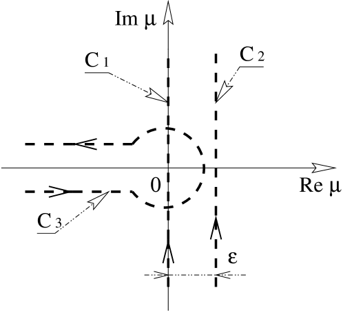
Figure A.1: Integration contours.

Now, since we shifted the contour, ${\rm Re}\mu>0$. Therefore each of the internal integrals in Eq. (A.15) is a $\Gamma$ function:

$${\cal I}=\prod_{j=1}^{K}\Gamma(z_{j}+1)\times\lim_{\varepsilon\to 0}\int_{C_{2}}\frac{d\mu}{2\pi i}\,\frac{{\rm e}^{\mu}}{\prod_{j}\mu^{z_{j}+1}}$$ (A.16)

In more complex cases we probably would have stopped here, trading $K$ real integrals of Eq. (A.13) for one contour integration in the complex plane—this is why this method may be of use. However, our toy model is very easy, so we can proceed further and do the $\mu$ integration. Remembering that $\varepsilon$ is small, we can now use the Jordan’s lemma and bend the integration contour $C_{2}$ into $C_{3}$. Then using a well known formula for the integral representation of the inverse $\Gamma$–function [Gradshtein and Ryzhik 1965, Eq. (8.315)] we get

$${\cal I}=\int_{0}^{1}dt_{1}\,dt_{2}\cdots dt_{K}\,\prod_{j=1}^{K}t^{z_{j}}\delta\left(1-\sum_{k=1}^{K}t_{k}\right)=\frac{\prod_{j=1}^{K}\Gamma(z_{j}+1)}{\Gamma(\sum_{j=1}^{K}z_{j}+K)}$$ (A.17)

Note that, in the case of Eq. (4.6), the sum of $z_{j}$’s is just $N$.

Bibliography

Abarbanel, H. D. I., Brown, R., Sidorowich, J. J., & Tsimring L. S. (1993). The analysis of observed chaotic data in physical systems, Revs. Mod. Phys. 65, 1331–1392.

Adami, C., & Cerf N. J. (2000). Physical complexity of symbolic sequences, Physica D 137, 62–69. See also adap-org/9605002.

Aida, T. (1999). Field theoretical analysis of on–line learning of probability distributions, Phys. Rev. Lett. 83, 3554–3557. See also cond-mat/9911474.

Akaike, H. (1974a). Information theory and an extension of the maximum likelihood principle, in Second international symposium of information theory, B. Petrov and F. Csaki, eds. Budapest: (Akademia Kiedo, Budapest).

Akaike, H. (1974b). A new look at the statistical model identification, IEEE Trans. Automatic Control. 19, 716–723.

Atick, J. J. (1992). Could information theory provide an ecological theory of sensory processing? In Princeton Lectures on Biophysics, W. Bialek, ed., pp. 223–289 (World Scientific, Singapore).

Attneave, F. (1954). Some informational aspects of visual perception, Psych. Rev. 61, 183–193.

Balasubramanian, V. (1997). Statistical inference, Occam’s razor, and statistical mechanics on the space of probability distributions, Neural Comp. 9, 349–368. See also cond-mat/9601030.

Barlow, H. B. (1959). Sensory mechanisms, the reduction of redundancy and intelligence, in Proceedings of the Symposium on the Mechanization of Thought Processes, vol. 2, D. V. Blake and A. M. Uttley, eds., pp. 537–574 (H. M. Stationery Office, London).

Barlow, H. B. (1961). Possible principles underlying the transformation of sensory messages, in Sensory Communication, W. Rosenblith, ed., pp. 217–234 (MIT Press, Cambridge).

Barlow, H. B. (1983). Intelligence, guesswork, language, Nature 304, 207–209.

Bennett, C. H. (1990). How to define complexity in physics, and why, in Complexity, Entropy and the Physics of Information, W. H. Zurek, ed., pp. 137–148 (Addison–Wesley, Redwood City).

Bialek, W. (1995). Predictive information and the complexity of time series, NEC Research Institute technical note.

Bialek, W., Callan, C. G., & Strong, S. P. (1996). Field theories for learning probability distributions, Phys. Rev. Lett. 77, 4693–4697. See also
cond-mat/9607180.

Bialek, W., Fairhall, A., Miller, J., & Nemenman, I., in preparation.

Bialek, W., Nemenman, I., & Tishby N. (2000). Predictability, complexity and learning, preprint. Available at physics/0007070.

Bialek, W., & Nemenman, I. (2000). Learning continuous distributions: simulations with field theoretic priors, in preparation.

Bialek, W., & Tishby, N. (1999). Predictive information, preprint. Available at cond-mat/9902341.

Bialek, W., & Tishby, N. (in preparation). Extracting relevant information.

Brenner, N., Bialek, W., & de Ruyter van Steveninck, R. (2000). Adaptive rescaling optimizes information transmission, Neuron 26, 695–702.

Bruder, S. D. (1998). Ph.D. Dissertation, Princeton University.

Capaldi, E. A.,  Robinson, G. E., & Fahrbach S. E. (1999). Neuroethology of spatial learning: The birds and the bees, Annu. Rev. Psychol. 50, 651–682.

Carpenter, R. H. S., & Williams, M. L. L. (1995). Neural computation of log likelihood in control of saccadic eye movements, Nature 377, 59–62.

Chaitin, G. J. (1975). A theory of program size formally identical to information theory, J. Assoc. Comp. Mach. 22, 329–340.

Clarke, B. S., & Barron A. R. (1990). Information–theoretic asymptotics of Bayes methods, IEEE Trans. Inf. Thy. 36, 453–471.

Clarke, B. S., & Barron A. R. (1994). Jeffreys’ prior is asymptotically least favorable under entropy risk, J. Stat. Planning and Inference 41, 37–60.

Coleman, S. (1988). Aspects of symmetry, (Cambridge University Press, Cambridge).

Cover, T. M., & King, R. C. (1978). A convergent gambling estimate of the entropy of English, IEEE Trans. Inf. Thy. 24, 413–421.

Cover, T. M., & Thomas, J. A. (1991). Elements of Information Theory (Wiley, New York).

Crutchfield, J. P., & Feldman, D. P. (1997). Statistical complexity of simple 1–d spin systems, Phys. Rev. E 55, 1239–1243R. See also cond-mat/9702191.

Crutchfield, J. P., Feldman, D. P., & Shalizi C. R. (1999). Comment on “Simple measure for complexity,” preprint. Available at chao-dyn/9907001.

Crutchfield, J. P., & Shalizi, C. R. (1998). Thermodynamic depth of causal states: objective complexity via minimal representation, Phys. Rev. E 59, 275–283. See also cond-mat/9808147.

Crutchfield, J. P., & Young, K. (1989). Inferring statistical complexity, Phys. Rev. Lett. 63, 105–108.

Ebeling, W., & Pöschel, T. (1994). Entropy and long-range correlations in literary English, Europhys. Lett. 26, 241–246.

Feldman, D. P., & Crutchfield, J. P. (1998). Measures of statistical complexity: why? Phys. Lett. A 238, 244–252. See also cond-mat/9708186.

Gell–Mann, M., & Lloyd, S. (1996). Information measures, effective complexity, and total information, Complexity 2, 44–52.

de Gennes, P.–G. (1979). Scaling Concepts in Polymer Physics (Cornell University Press, Ithaca and London).

Gradshtein, I. S., Ryzhik I. M., (1965). Tables of integrals, series, and products, 4th ed. (Academic Press, New York).

Grassberger, P. (1986). Toward a quantitative theory of self–generated complexity, Int. J. Theor. Phys. 25, 907–938.

Haussler, D., Kearns, M., Seung, S., & Tishby, N. (1996). Rigorous learning curve bounds from statistical mechanics, Machine Learning 25, 195–236.

Hawken, M. J., & Parker, A. J. (1991). Spatial receptive field organization in monkey V1 and its relationship to the cone mosaic, in Computational models of visual processing, M. S. Landy and J. A.  Movshon, eds., pp. 83–93 (MIT Press, Cambridge)

van Helden, J., Andre, B., & Collado-Vides, J. (1998). Extracting regulatory sites from the upstream region of yeast genes by computational analysis of oligonucleotide frequencies, J. Mol. Biol., 281, 827–842.

Herschkowitz, D., & Nadal, J.–P. (1999). Unsupervised and supervised learning: mutual information between parameters and observations, Phys. Rev. E, 59, 3344–3360.

Hilberg, W. (1990). The well–known lower bound of information in written language: Is it a misinterpretation of Shannon experiments? (in German) Frequenz 44, 243–248.

Holy, T. E. (1997). Analysis of data from continuous probability distributions, Phys. Rev. Lett. 79, 3545–3548. See also physics/9706015.

Kemeney, J. G. (1953). The use of simplicity in induction, Philos. Rev. 62, 391–315.

Knudsen, E. I., du Lac S., & Esterly S. D. (1987). Computational maps in brain, Ann. Rev. Neurosci. 10, 41–65.

Kolmogoroff, A. (1939).  Sur l’interpolation et extrapolations des suites stationnaires, C. R. Acad. Sci. Paris 208, 2043–2045.

Kolmogorov, A. N. (1941). Interpolation and extrapolation of stationary random sequences (in Russian), in Izv. Akad. Nauk. SSSR Ser. Mat. 5, 3–14; translation in Selected Works of A. N. Kolmogorov, vol. II. A. N. Shiryagev, ed., pp. 272–280 (Kluwer Academic Publishers, Dordrecht, The Netherlands).

Kolmogorov, A. N. (1965). Three approaches to the quantitative definition of information, Prob. Inf. Trans. 1, 4–7.

Li, M., & Vitányi, P. (1993). An Introduction to Kolmogorov Complexity and its Applications (Springer-Verlag, New York).

Lloyd, S., & Pagels, H. (1988). Complexity as thermodynamic depth, Ann. Phys. 188, 186–213.

Logothetis, N. K., & Sheinberg, D. L. (1996). Visual object recognition, Annu. Rev. Neurosci. 19, 577–621.

Lopes, L. L., & Oden, G. C. (1987). Distinguishing between random and nonrandom events, J. Exp. Psych.: Learning, Memory, and Cognition 13, 392–400.

Lopez–Ruiz, R., Mancini, H. L., & Calbet, X. (1995). A statistical measure of complexity, Phys. Lett. A 209, 321–326.

MacKay, D. J. C. (1992). Bayesian interpolation, Neural Comp. 4, 415–447.

Manning C., & Schütze H. (1999). Foundations of statistical natural language processing (MIT Press, Cambridge, MA).

Opper, M. (1994). Learning and generalization in a two-layer neural network: the role of the Vapnik–Chervonenkis dimension, Phys. Rev. Lett. 72, 2113–2116.

Opper, M., & Haussler, D. (1995). Bounds for predictive errors in the statistical mechanics of supervised learning, Phys. Rev. Lett. 75, 3772–3775.

Pereira F., Tishby N., & Lee L. (1993). Distributional clustering of English words, in Proceedings of the 31st Annual Meeting of the Association for Computational Linguistics, pp. 183–190.

Periwal, V. (1997). Reparametrization invariant statistical inference and gravity, Phys. Rev. Lett. 78, 4671–4674. See also hep-th/9703135.

Periwal, V. (1998). Geometrical statistical inference, Nucl. Phys. B 554[FS], 719–730. See also adap-org/9801001.

Pöschel, T., Ebeling, W., & Rosé, H. (1995). Guessing probability distributions from small samples, J. Stat. Phys. 80, 1443–1452.

Press, W., Flannery, B., Teukolsky S., Vetterling, W. (1988) Numerical recipes in C (Cambridge University Press , Cambridge).

Rieke, F., Warland, D., de Ruyter van Steveninck, R., & Bialek, W. (1997). Spikes: Exploring the Neural Code (MIT Press, Cambridge).

Rissanen, J. (1978). Modeling by shortest data description, Automatica, 14, 465–471.

Rissanen, J. (1983). A universal prior for integers and estimation by minimum description length, Ann. Stat. 11, 416–431.

Rissanen, J. (1984). Universal coding, information, prediction, and estimation, IEEE Trans. Inf. Thy. 30, 629–636.

Rissanen, J. (1986). Stochastic complexity and modeling, Ann. Statist. 14, 1080–1100.

Rissanen, J. (1987). Stochastic complexity, J. Roy. Stat. Soc. B, 49, 223–239, 253–265.

Rissanen, J. (1989). Stochastic Complexity and Statistical Inquiry (World Scientific, Singapore).

Rissanen, J. (1996). Fisher information and stochastic complexity, IEEE Trans. Inf. Thy. 42, 40–47.

Saffran, J. R., Aslin, R. N., & Newport, E. L. (1996). Statistical learning by 8–month–old infants, Science 274, 1926–1928.

Saffran, J. R., Johnson, E. K., Aslin, R. H., & Newport, E. L. (1999). Statistical learning of tone sequences by human infants and adults, Cognition 70, 27–52.

Seung, H. S., Sompolinsky, H., & Tishby, N. (1992). Statistical mechanics of learning from examples, Phys. Rev. A 45, 6056–6091.

Shalizi, C. R., & Crutchfield, J. P. (1999). Computational mechanics: pattern and prediction, structure and simplicity, preprint. Available at
cond-mat/9907176.

Shalizi, C. R., & Crutchfield, J. P. (2000). Information bottleneck, causal states, and statistical relevance bases: how to to represent relevant information in memoryless transduction. Available at nlin.AO/0006025.

Shiner, J., Davison, M., & Landsberger, P. (1999). Simple measure for complexity, Phys. Rev. E 59, 1459–1464.

Shannon, C. E. (1948). A mathematical theory of communication, Bell Sys. Tech. J. 27, 379–423, 623–656. Reprinted in C. E. Shannon and W. Weaver, The Mathematical Theory of Communication (University of Illinois Press, Urbana, 1949).

Shannon, C. E. (1951). Prediction and entropy of printed English, Bell Sys. Tech. J. 30, 50–64. Reprinted in N. J. A. Sloane and A. D. Wyner, eds., Claude Elwood Shannon: Collected papers (IEEE Press, New York, 1993).

Smirnakis, S., Berry III, M. J., Warland, D. K., Bialek, W., & Meister, M. (1997). Adaptation of retinal processing to image contrast and spatial scale, Nature 386, 69–73.

Sole, R. V., & Luque, B. (1999). Statistical measures of complexity for strongly interacting systems, preprint. Available at adap-org/9909002.

Solomonoff, R. J. (1964). A formal theory of inductive inference, Inform. and Control 7, 1–22, 224–254.

Tishby, N., Pereira, F., & Bialek, W. (1999). The information bottleneck method, in Proceedings of the 37th Annual Allerton Conference on Communication, Control and Computing, B. Hajek and R. S. Sreenivas, eds., pp. 368–377 (University of Illinois). See also physics/0004057

Vapnik, V. (1998). Statistical Learning Theory (John Wiley & Sons, New York).

Vitányi, P., & Li, M. (2000). Minimum description length induction, Bayesianism, and Kolmogorov Complexity, IEEE Trans. Inf. Thy. 46, 446–464. See also cs.LG/9901014.

Weigend, A. S., & Gershenfeld, N. A., eds. (1994). Time series prediction: Forecasting the future and understanding the past (Addison–Wesley, Reading MA).

Wiener, N. (1949). Extrapolation, Interpolation and Smoothing of Time Series (Wiley, New York).