Time-Symmetric ADI and Causal Reconnection: Stable Numerical Techniques for Hyperbolic Systems on Moving Grids.

Abstract

Moving grids are of interest in the numerical solution of hydrodynamical problems and in numerical relativity. We show that conventional integration methods for the simple wave equation in one and more than one dimension exhibit a number of instabilities on moving grids. We introduce two techniques, which we call causal reconnection and time-symmetric ADI, which together allow integration of the wave equation with absolute local stability in any number of dimensions on grids that may move very much faster than the wave speed and that can even accelerate. These methods allow very long time-steps, are fully second-order accurate, and offer the computational efficiency of operator-splitting.

We develop causal reconnection first in the one-dimensional case: we find that a conventional implicit integration scheme that is unconditionally stable as long as the speed of the grid is smaller than that of the waves nevertheless turns unstable whenever the grid speed increases beyond this value. We introduce a notion of local stability for difference equations with variable coefficients. We show that, by “reconnecting” the computational molecule at each time-step in such a way as to ensure that its members at different time-steps are within one another’s causal domains, one eliminates the instability, even if the grid accelerates. This permits very long time-steps on rapidly moving grids. The method extends in a straightforward and efficient way to more than one dimension.

However, in more than one dimension, it is very desirable to use operator-splitting techniques to reduce the computational demands of implicit methods, and we find that standard schemes for integrating the wave equation — Lees’ First and Second Alternating Direction Implicit (ADI) methods — go unstable for quite small grid velocities. Lees’ first method, which is only first-order accurate on a shifting grid, has mild but nevertheless significant instabilities. Lees’ second method, which is second-order accurate, is very unstable.

By adopting a systematic approach to the design of ADI schemes, we develop a new ADI method that cures the instability for all velocities in any direction up to the wave speed. This scheme is uniquely defined by a simple physical principle: the ADI difference equations should be invariant under time-inversion. (The wave equation itself and the full implicit difference equations satisfy this criterion, but neither of Lees’ methods do.) This new time-symmetric ADI scheme is, as a bonus, second-order accurate. It is thus far more efficient than a full implicit scheme, just as stable, and just as accurate.

By implementing causal reconnection of the computational molecules, we extend the time-symmetric ADI scheme to arrive at a scheme that is second order accurate, computationally efficient and unconditionally locally stable for all grid speeds and long time-steps. We have tested the method by integrating the wave equation on a rotating grid, where it remains stable even when the grid speed at the edge is 15 times the wave speed. Because our methods are based on simple physical principles, they should generalize in a straightforward way to many other hyperbolic systems. We discuss briefly their application to general relativity and their potential generalization to fluid dynamics.

I Introduction.

In the numerical study of wave phenomena it is often necessary to use a reference frame that is moving with respect to the medium in which the waves propagate. This could be the case, for example, when studying the waves generated by a moving source, where it may prove convenient to use a reference frame attached to this source. In some cases, one may even need to use a frame that moves faster than the waves themselves, as in the case of a supersonic flow. In general relativity, especially in black-hole problems, one may have to use a grid that shifts rapidly, even faster than light. All these problems arise in more than one spatial dimension, where computational efficiency may make stringent demands on the algorithm. It is a common experience to find that standard algorithms seem to go unstable in realistic problems. In this paper, by studying the simple wave equation, we show that the consistent application of two fundamental physical principles — causality and time-reversal-invariance — produces remarkably stable, efficient and accurate integration methods. These principles can easily be applied to more complex physical systems, where we would expect similar benefits.

Our principal motivation for studying these techniques is the development of suitable algorithms for the numerical simulation of moving, interacting black holes. Relativists have long acknowledged the importance of using shifting grids in some problems, but to our knowledge there has been no systematic study of the effects of such shifts on the stability of numerical algorithms. In the next two paragraphs we develop this motivation. Readers not concerned with numerical relativity may skip these without loss of continuity.

Let us consider the requirements that black-hole problems will make of our algorithms. Within the context of the  $3+1$  formalism of General Relativity ([1], [2]), it would seem to be desirable to develop methods on a quasi-rectangular 3-dimensional grid, so that no special coordinate features would prevent one from studying quite general problems. If we imagine a picture in which a black hole moves “through” such a grid, much the way a star would if it were interacting with another, then some requirements become clear:

1. Grid points will move from outside to inside the horizon, but the grid as a whole should not be sucked in. This may require an inner boundary to the grid, say on a marginally trapped surface, and this boundary will have to move at faster than the speed of light. Grid points may cross this boundary and be forgotten, at least temporarily, but others will emerge on the other side of the boundary.

2. Grid points that so emerge will then move from inside to outside the horizon as the hole passes over them; this will require grids that shift faster than light. This is inescapable unless one ties the grid to the hole as it moves.

3. If two black holes begin in orbit around one another, then it may be desirable to adopt a grid that rotates with respect to infinity, in which the holes move relatively slowly at first. In such a grid one would expect that one could take long time-steps without losing accuracy, since not much happens initially. One therefore would like to be free of the Courant condition on time-steps, i.e. one wants to use implicit methods.

4. Integrating the equations of general relativity on a grid with reasonable resolution will tax the capacity of the best available computers for some time to come. Full implicit schemes are very time-consuming in more than one spatial dimension, because they require the inversion of huge sparse matrices. Alternating-direction-implicit (ADI) schemes reduce this burden enormously by turning the integration into a succession of one-dimensional implicit integrations, so an ADI scheme that can cope with grid shifts is very desirable.

In this paper we show that it should be possible to develop stable methods that satisfy the last three requirements above: ADI schemes that are absolutely stable and computationally efficient even on grids that shift at many times the speed of light. As a bonus, our ADI methods preserve the second-order accuracy of the full implicit equations. The first requirement, that of dealing with an inner boundary that moves faster than light, is closely related to these techniques and will be addressed elsewhere.

Having these requirements in mind, we have studied the effects that the use of a moving reference frame has on the finite difference approximation to the simple wave equation, centering our attention particularly in the stability properties. The wave equation is the simplest system, so the instabilities we find in the standard ADI methods should certainly also be present when they are applied to more realistic physical systems. Of course, the wave equation is much simpler than other systems, so it is possible that methods that stabilize its integration will not extend to other systems. However, the principles that we find here are of such a fundamental physical nature that it seems certain that they should be applied wherever possible. Other kinds of instabilities may of course arise in complex systems, especially those directly due to nonlinearity, but we feel that moving-grid instabilities are likely to be cured by the methods we describe here.

We shall conclude this introductory section by summarizing the approach and results of the following sections. In the second section we develop the mathematical framework of shifting grids. Then in Section III we study the one-dimensional wave equation. We find simple implicit finite difference schemes that are locally stable for any speed up to that of the waves, even when the grid is accelerating as well as moving. When formulated on a grid that is moving, and even accelerating, it is not immediately obvious how one defines stability: solutions of the differential equation do not have simple harmonic time-dependence in this frame. We find that a satisfactory criterion for local stability of these simple schemes is that no solutions of the difference equations should grow faster anywhere on the grid than local solutions of the differential equation.

However, as soon as the reference frame moves faster than the wave speed, these schemes become highly unstable. We trace the origin of this instability to the fact that the computational molecules no longer represent in an adequate way the causal relationships between the grid points. We find that by modifying the molecules so that they link a given point on one time-slice with one on the next one that is within the first point’s cone of characteristics (its forward “light cone”), one can restore stability. We discuss one algorithm for doing this in Appendix B.

We call this causal reconnection. It is important to note that this has a minimal impact on the integration scheme: for implicit schemes, the matrix that must be solved for the solution at a given time-step is constructed only from the relations between grid-points at that time-step, while causal reconnection affects only the relations between points on different time-steps. Thus, it can be incorporated into the part of the algorithm that constructs the “inhomogeneous terms” that generate the right-hand-side of the implicit matrix equation. For the 1-dimensional wave equation, the extra work involved in seeking out causally related grid points can be significant, but it becomes a smaller proportion of the overhead in more than one dimension, and for complicated systems of equations, such as one has in general relativity, the overhead will be a negligible fraction of the total work per time-step. We have tested causal reconnection and found it to be stable even on grids moving at many times the speed of the waves. It is also insensitive to the acceleration of the grid.

We then move our attention in Section IV to operator-splitting ADI methods [4], which are computationally efficient ways of implementing implicit schemes in more than one dimension. We find it helpful to derive ADI schemes from a more systematic point of view than one usually finds in expositions of this technique. The goal is to add extra terms to a set of difference equations that (i) do not change its accuracy, but (ii) replace the large sparse non-tridiagonal matrix which has to be solved in implicit schemes with a matrix that is a simple product of tridiagonal matrices of the 1-D implicit form for each dimension, which are easy to solve. The extra terms are related to the “left-over” terms that appear as the difference between the true operator and its factored replacement acting on the data values on the final time-step. These final-time-step terms must be eliminated. They are in effect replaced by similar terms from earlier time-steps, which replacement makes no difference when $\Delta t\rightarrow 0$, but which removes them from the matrix inversion and allows them to be included as part of the inhomogeneous terms in the matrix solution. Then the new equations will be a valid approximation to the differential equation but can be solved by a succession of (rapid) 1-D tridiagonal matrix solutions.

When subjected to the same stability analysis as we devised for causal reconnection, the standard ADI methods show instabilities even when the reference frame moves very slowly. The instability is most marked in Lees’ second method, in which the extra terms added in are of second order and therefore do not degrade the accuracy of the full implicit scheme. The instability is also present, albeit more weakly, in Lees’ first scheme, which is only first-order accurate.

We trace these instabilities to the fact that the extra terms added in either of the standard methods break the time-reversal invariance exhibited by the original differential equation and by the full implicit difference equations. Demanding that the extra terms be time-symmetric uniquely determines an ADI scheme that is essentially a hybrid of Lees’ first and second methods. This time-symmetric ADI method turns out to be fully stable for all grid shifts up to the wave speed. Although not built in as a requirement, the new method also turns out to be second-order accurate.

The method can then be extended to grid speeds larger than the wave speed by a direct generalization of the causal reconnection approach developed for the one-dimensional case. We demonstrate this by performing an integration on a rotating grid whose edge moves faster than the wave speed.

In Appendix A, we derive the wave equation in the accelerating coordinate system using the efficient tensorial techniques of relativity. In Appendix B, we discuss one method of implementing causal reconnection.

II The wave equation on a moving grid.

The wave equation is a good testing ground for any new algorithms for hyperbolic systems. The equations governing many wave systems can be reduced to the standard wave equation, and its cone of characteristics has the causal structure of space-time. We shall use it to test methods for integrating hyperbolic systems on moving grids.

We consider the wave equation in an arbitrary number of spatial dimensions  $n$ ,

$$\nabla^{2}\phi-\frac{1}{c^{2}}\frac{\partial^{2}\phi}{\partial t^{2}}\,=\,0\,.$$ (II.1)

written in a standard inertial coordinate system denoted by  ($t,\xi^{i}$).

We are interested in finding a finite difference approximation to this equation using a grid of points that moves with an arbitrary non-uniform speed. Moreover, we will assume that the speed of each grid point can change with time. In order to represent this situation, we need to introduce a second coordinate system $(t,x^{i})$ that will be comoving with the grid. We introduce these coordinates in the continuous case by a transformation of the form

$$x^{i}\,=\,x^{i}(t,\,\xi^{k})\,.$$ (II.2)

We have not changed the time coordinate, so we assume that the identification of surfaces of constant time does not change. This is thus not the usual Lorentz transformation of special relativity, so there is no reason for the form of the wave equation to remain invariant. This will have the implication that, in finite differences, the time interval between $t=\rm const$ slices will be constant, independent of position. For problems in general relativity, this is somewhat of a restriction, but we do not feel it is a serious one. If the causal relations are properly taken into account, then a spatial dependence in the lapse function ought not to change our physical conclusions.

In Appendix A we show that the wave equation takes the following form in the new coordinates $(t,x^{i})$:

$$(g^{i\,k}-\beta^{i}\beta^{k})\,\frac{\partial^{2}\phi}{\partial x^{i}\,\partial x^{k}}+\frac{2\beta^{i}}{c}\,\frac{\partial^{2}\phi}{\partial x^{i}\,\partial t}-\Gamma^{i}\,\frac{\partial\phi}{\partial x^{i}}-\frac{1}{c^{2}}\,\frac{\partial^{2}\phi}{\partial t^{2}}\,=\,0\,.$$ (II.3)

The following quantities derived from the coordinate transformation appear in the last equation:

$$\beta^{i} := \,-\frac{1}{c}\,\frac{\partial x^{i}}{\partial t}\,,$$ (II.4)

$$g_{\,i\,j} := \sum_{l=1}^{n}\,\frac{\partial\xi^{l}}{\partial x^{i}}\,\frac{\partial\xi^{l}}{\partial x^{j}}\rule[0.0pt]{0.0pt}{22.76219pt}\,,$$ (II.5)

$$g^{\,i\,j} := \sum_{l=1}^{n}\,\frac{\partial x^{i}}{\partial\xi^{l}}\,\frac{\partial x^{j}}{\partial\xi^{l}}\,,$$ (II.6)

$$g := \det\left(g_{ij}\right)\rule[0.0pt]{0.0pt}{17.07164pt}\,,$$ (II.7)

$$\Gamma^{i} := -\frac{1}{\sqrt{g}}\left\{\frac{\partial}{\partial t}\left(\sqrt{g}\beta^{i}\right)+\frac{\partial}{\partial x^{j}}\left[\sqrt{g}\left(g^{ij}-\beta^{i}\beta^{j}\right)\right]\right\}\rule[0.0pt]{0.0pt}{25.60747pt}\,.$$ (II.8)

Each of these quantities has a physical interpretation, which we now explain. Readers familiar with these ideas may skip to the next section.

The shift vector  $\beta^{i}$  gives the relationship between the two coordinate systems on nearby surfaces of constant time. Let the line of constant  $\{\xi^{i}\}$  have coordinates  $\{x^{i}_{t}\}$  at the lower hypersurface and  $\{x^{i}_{t+dt}\}$ at the upper hypersurface. From the definition of the shift vector in Equation II.4, it is clear that

$$x^{i}(\xi^{j},t+dt)\,\approx\,x^{i}(\xi^{j},t)\,-\,c\,\beta^{i}dt\,.$$ (II.9)

As we illustrate in Figure 1, if one starts at any given point at time $t$, then by time $t+dt$ the $\{x^{i}\}$ coordinates will have shifted by an amount equal to the shift vector times $c\,dt$ relative to the $\{\xi^{i}\}$ (inertial) coordinates. The shift vector  $\beta^{i}$  will in general be a function of both  $\{x^{i}_{t}\}$  and t.

FIG. 1.: Shift vector $\beta^{i}$.

We now introduce the spatial metric tensor  $g_{\,i\,j}$, which we have defined in Equation II.5. Its name comes from the fact that the distance  $dl$  between two points whose coordinates differ by $d\xi^{l}$ in the original coordinates and by  $dx^{i}$  in the shifting coordinates is given by the Pythagorean Theorem:

$$dl^{\,2}\,=\,\sum_{l=1}^{n}d\xi^{l}\,d\xi^{l}=\sum_{i,j=1}^{n}g_{\,i\,j}\,dx^{i}dx^{j}$$ (II.10)

That this gives Equation II.5 for $g_{ij}$ is readily seen by substituting the following transformation from $d\xi^{l}$ to $dx^{i}$ into the first version of the Pythagorean Theorem:

$$d\xi^{l}=\sum_{i=1}^{n}\frac{\partial\xi^{l}}{\partial x^{i}}dx^{i}.$$ (II.11)

The next tensor that appears in the general form of the wave equation is the inverse metric tensor given by Equation II.6. This is the matrix inverse of the metric tensor,

$$\sum_{j=1}^{n}g^{ij}g_{jk}=\delta^{i}_{k},$$ (II.12)

as can easily be seen by substituting Equations II.5 and II.6 into the above.

The final quantity we need is $\Gamma^{i}$, a measure of the acceleration of the shifting coordinates with respect to the old ones, given by Equation II.8. We will leave the full derivation of $\Gamma^{i}$ to Appendix A, but to illustrate our interpretation of it as an acceleration term, we shall explicitly evaluate it in the case where the new coordinates are obtained from the inertial ones by a simple shift independent of position. Then the shift vector  $\beta^{i}$  is only a function of time, and the spatial metric  $g_{\,i\,j}$  is just the unit matrix:

$$\frac{\partial\beta^{i}}{\partial x^{j}}\,=\,0\,,\hskip 28.45274ptg_{\,i\,j}\,=\,\delta_{\,i\,j}\,.$$ (II.13)

It is not difficult to see that in this case the coefficients  $\Gamma^{i}$  reduce to:

$$\Gamma^{i}\,=\,-\,\frac{1}{c}\,\frac{d\beta^{i}}{dt}\,.$$ (II.14)

Since the shift vector gives the speed of the $\{x^{i}\}$ coordinates, the last expression implies that the  $\Gamma^{i}$  coefficients are essentially the acceleration.

Notice that if there is no acceleration, the only essential difference from the normal wave equation is the transport term $\vec{\beta}\cdot\nabla\dot{\phi}$, which arises as well in hydrodynamical problems. We will see that the local stability properties of the algorithms we study are determined mainly by $\beta^{i}$, not $\Gamma^{i}$, which is one reason we expect our analysis to have much wider applicability than just to problems involving the wave equation.

Having derived the form of the wave equation in our new coordinates, we now establish a grid for formulating difference equations in these coordinates. By assumption, we take the time-interval $\Delta t$ between successive surfaces of constant time to be uniform (independent of position) and constant (the same for any pair of surfaces). We take each grid point to have a fixed spatial coordinate position $x^{i}$, and for convenience we take the spacing between grid points $\Delta x^{i}$ to be uniform in each coordinate direction. As seen in the inertial frame, the grid deforms itself as in Figure 2. The corresponding picture in the $x^{i}$-coordinate frame looks much more regular (Figure 3).

FIG. 2.: Grid in original coordinates, showing true distances.

FIG. 3.: Grid in new coordinates.

III The one dimensional case.

A Finite difference approximation.

The one-dimensional wave equation allows us to study shifting grids in a relatively simple fashion. The added complication of extra dimensions will be treated in the next section.

In one spatial dimension, the metric, shift, and acceleration coefficients reduce to scalar functions:

$$\left.\begin{array}[]{lll}g_{\,1\,1}(x,t)\,=\,g(x,t)\,,\\ \\ \beta^{1}(x,t)\,=\,\beta(x,t)\,,\\ \\ \Gamma^{1}(x,t)\,=\,\Gamma(x,t)\,.\end{array}\right\}$$ (III.1)

Because the metric scales the squares of the coordinate distances (Equation II.10), it is convenient to define the linear scale function  $s(x,t)$  by

$$s(x,t)\,:=\,\sqrt{g(x,t)}=\frac{\partial\xi}{\partial x}\,,$$ (III.2)

so that the spatial proper distance is given by

$$d\xi\,=\,s(x,t)\,dx\,.$$ (III.3)

Using this expression, Equation II.3 becomes:

$$(\frac{1}{s^{2}}-\beta^{2})\,\frac{\partial^{2}\phi}{\partial x^{2}}+\frac{2\beta}{c}\,\frac{\partial^{2}\phi}{\partial x\,\partial t}-\Gamma\,\frac{\partial\phi}{\partial x}-\frac{1}{c^{2}}\,\frac{\partial^{2}\phi}{\partial t^{2}}\,=\,0\,.$$ (III.4)

For the finite difference approximation to this equation we employ the usual notation:

$$\phi^{j}_{i}\,:=\,\phi\,(i\,\Delta x,j\,\Delta t)\,.$$ (III.5)

We define the first and second centered spatial differences as:

$$\left.\begin{array}[]{ll}\delta_{x}\,\phi^{j}_{i}\,:=\,\phi^{j}_{i+1}-\phi^{j}_{i-1}\,,\\ \\ \delta^{2}_{x}\,\phi^{j}_{i}\,:=\,\phi^{j}_{i+1}-2\phi^{j}_{i}+\phi^{j}_{i-1}\,.\end{array}\right\}$$ (III.6)

It is important to note that with the last definitions $\left(\delta_{x}\right)^{2}\,\neq\,\delta^{2}_{x}$. We can also define analogous differences for the time direction.

We now write the finite difference approximation to the differential operators that appear in Equation III.4 using the computational molecule shown in Figure 4. We have:

$$\left(\partial^{2}_{t}\,\phi\right)^{j}_{i}\,=\,\frac{\phi^{j+1}_{i}-2\phi^{j}_{i}+\phi^{j-1}_{i}}{\left(\Delta t\right)^{2}}+E_{tt}\,,$$ (III.7)

where  $E_{tt}$  is the truncation error whose principal part is:

$$E_{tt}\,=\,-\frac{\left(\Delta t\right)^{2}}{12}\,\left(\partial^{4}_{t}\,\phi\right)^{j}_{i}\,+\ldots\,.$$ (III.8)

Similarly, for the mixed derivative in space and time we find:

$$\left(\partial_{x}\partial_{t}\,\phi\right)^{j}_{i}\,=\,\frac{\delta_{x}\,\phi^{j+1}_{i}-\delta_{x}\,\phi^{j-1}_{i}}{4\,\Delta x\,\Delta t}+E_{xt}\,,$$ (III.9)

with:

$$E_{xt}\,=\,-\frac{1}{6}\left[\left(\Delta x\right)^{2}\,\left(\partial^{3}_{x}\partial_{t}\,\phi\right)^{j}_{i}+\left(\Delta t\right)^{2}\,\left(\partial_{x}\partial^{3}_{t}\,\phi\right)^{j}_{i}\right]\,+\,\ldots\,.$$ (III.10)

FIG. 4.: Computational molecule.

For the second derivative in the  $x$  direction we use an implicit approximation of the following form:

$$\left(\partial^{2}_{x}\phi\right)^{j}_{i}=\frac{\theta_{1}}{2}\,\left[\frac{\delta^{2}_{x}\,\phi^{j+1}_{i}}{\left(\Delta x\right)^{2}}+\frac{\delta^{2}_{x}\,\phi^{j-1}_{i}}{\left(\Delta x\right)^{2}}\right]+\left(1-\theta_{1}\right)\,\left[\frac{\delta^{2}_{x}\,\phi^{j}_{i}}{\left(\Delta x\right)^{2}}\right]+E_{xx}\,,$$ (III.11)

where  $\theta_{1}$  is an arbitrary parameter that gives the weight of the implicit terms. If  $\theta_{1}\,=\,0$  the approximation is explicit, while if  $\theta_{1}\,=\,1$  all the weight is given to the initial and final time-steps of the molecule in the figure. Note that the last equation is symmetric in time. The error for this  $x$  derivative is:

$$E_{xx}\,=\,-\frac{\left(\Delta x\right)^{2}}{12}\,\left(\partial^{4}_{x}\,\phi\right)^{j}_{i}-\theta_{1}\,\frac{\left(\Delta t\right)^{2}}{2}\,\left(\partial^{2}_{x}\partial^{2}_{t}\,\phi\right)^{j}_{i}\,+\,\ldots\,.$$ (III.12)

Finally, for the first derivative in  $x$  we take:

$$\left(\partial_{x}\,\phi\right)^{j}_{i}\,=\,\frac{\theta_{2}}{2}\left[\frac{\delta_{x}\,\phi^{j+1}_{i}}{2\,\Delta x}\,+\,\frac{\delta_{x}\,\phi^{j-1}_{i}}{2\,\Delta x}\right]\,+\,\left(1-\theta_{2}\right)\,\left[\frac{\delta_{x}\,\phi^{j}_{i}}{2\,\Delta x}\right]\,+\,E_{x}\,,$$ (III.13)

where we have used again an implicit approximation with a different parameter  $\theta_{2}$ . The truncation error  $E_{x}$  is:

$$E_{x}\,=\,-\left[\frac{\left(\Delta x\right)^{2}}{6}\,\left(\partial^{3}_{x}\,\phi\right)^{j}_{i}\,+\,\theta_{2}\,\frac{\left(\Delta t\right)^{2}}{2}\,\left(\partial_{x}\partial_{t}^{2}\,\phi\right)^{j}_{i}\right]\,+\,\ldots\,.$$ (III.14)

We can now write down a second order finite difference approximation to Equation III.4:

$$\rho^{2}\,\left(\frac{1}{s^{2}}-\beta^{2}\right)\,\left\{\frac{\theta_{1}}{2}\,\left[\delta^{2}_{x}\,\phi^{j+1}_{i}+\delta^{2}_{x}\,\phi^{j-1}_{i}\right]+\left(1-\theta_{1}\right)\,\left[\delta^{2}_{x}\,\phi^{j}_{i}\right]\right\}\,$$ (III.15)

$${}+\frac{\rho\beta}{2}\,\left[\delta_{x}\,\phi^{j+1}_{i}\,-\,\delta_{x}\,\phi^{j-1}_{i}\right]\,-\,\left[\phi^{j+1}_{i}-2\phi^{j}_{i}+\phi^{j-1}_{i}\right]\,$$ (III.16)

$${}-\frac{\rho\,\left(c\,\Delta t\right)}{2}\>\>\Gamma\,\left\{\frac{\theta_{2}}{2}\left[\delta_{x}\,\phi^{j+1}_{i}\,+\,\delta_{x}\,\phi^{j-1}_{i}\right]\,+\,\left(1-\theta_{2}\right)\,\left[\delta_{x}\,\phi^{j}_{i}\right]\right\}\, = \,0\,,$$ (III.17)

where  $\rho$  is the ‘Courant parameter’ [3] given by:

$$\rho\,:=\,\frac{c\,\Delta t}{\Delta x}\,.$$ (III.18)

The coefficients {$s$, $\beta$, $\Gamma$} appearing in Equation III.17 should be evaluated at the point  $\left(i,j\right)$  that corresponds to the center of the molecule.

To arrive at the final form of the difference equation we multiplied it through by  $\left(\Delta t\right)^{2}$ . This means that the overall truncation error is now

$$E_{\mbox{\ref{eq:finite1D}}}={\cal O}\left[\left(\Delta x\right)^{2}\,\left(\Delta t\right)^{2}\right]\,+\,{\cal O}\left[\left(\Delta t\right)^{4}\right]\,.$$ (III.19)

Equation III.17 is well studied in the particular case when  $\beta\,=\,\Gamma\,=\,0$  and  $s\,=\,1$  [4]. It is important to note that, because we use centered differences in the transport term, the above finite difference approximation will be implicit whenever the shift vector is different from zero, even when  $\theta_{1}\,=\,\theta_{2}\,=\,0$ . Therefore the use of implicit approximations for the spatial derivatives does not add any extra numerical difficulty.

We shall need to know how much numerical work is involved in using the implicit scheme. Suppose there are $N$ spatial grid points. Then Equation III.17 is to be solved for the $N$ values $\{\phi^{j+1}_{i},\,i=1,\ldots,N\}$ at the final time-step. The equation for index $i$ relates three such values, at points $\{i-1,\,i,\,i+1\}$. The system of equations therefore has the matrix form

$$\hat{\cal Q}_{x}\,\phi^{j+1}=f(\phi^{j},\,\phi^{j-1}),$$ (III.20)

where $\hat{\cal Q}_{x}$ is a tridiagonal $N\times N$ matrix, and the inhomogeneous term $f$ is constructed from field values at the first two time-steps. Solving a tridiagonal matrix involves  ${\cal O}\left(N\right)$  operations. Since we also need  ${\cal O}\left(N\right)$  operations for the solution of an explicit scheme, we see that the use of an implicit method in one dimension will increase the number of operations per time-step by at most a multiplier, independent of the number of grid points. Against this, the implicit scheme for certain choices of $\theta_{1}$ and $\theta_{2}$ can, on a fixed grid, take much larger time-steps, limited only by accuracy considerations. In the next section, we shall show that this property of the implicit scheme in one dimension can, with suitable modifications, be extended to grids that shift essentially arbitrarily fast.

B Local stability:   definition and analysis of the implicit scheme on a shifting grid.

It is well known [4] that the implicit approximation to the wave equation can be made unconditionally stable in the case when  $\beta\,=\,\Gamma\,=\,0$  and  $s\,=\,1$  by using an implicit parameter  $\theta_{1}\,\geq\,1/2$ . We are interested in studying under what conditions this property is preserved in the case of a shifting grid. The shifting grid introduces a major difficulty: the coefficients in the equation generally depend on both position and time. This complicates the definition of stability.

This difficulty means that an analytic stability analysis must be local: we will actually only consider the stability of the difference equation obtained from Equation III.17 by, at each point $(x,t)$, taking the coefficients to be constant, with the values corresponding to that point. We feel that this is not a very restrictive assumption, since in practice instabilities usually appear as local phenomena [4], with the fastest growing modes having wavelengths comparable to the grid spacing. Moreover, if the coefficients in the difference equation are not practically constant over a few grid points, then we are probably not approximating the original differential equation adequately anyway.

We will start then by considering the nature of the solutions of the differential equation in a very small region around the point  $\left(x,t\right)$ . As usual, we look for a solution of the form:

$$\phi(x,t)\,=\,e^{\imath\alpha t}\,e^{\imath kx}\,.$$ (III.21)

Substituting this in Equation III.4 gives the following “dispersion relation” for $\alpha$:

$$\alpha_{\pm}\,=\,k\beta c\pm c\,\left[\frac{k^{2}}{s^{2}}+ik\Gamma\right]^{1/2}\,.$$ (III.22)

The general solution for a wavenumber $k$ is

$$\phi(x,t)=e^{\imath kx}\left[Z_{+}e^{\imath\alpha_{+}t}+Z_{-}e^{\imath\alpha_{-}t}\right].$$ (III.23)

Clearly, if $\Gamma\neq 0$, then one of the independent solutions will grow with time, but the other one will decay because of what we shall call the analytic boundedness condition:

$$\left|e^{\imath\alpha_{+}t}e^{\imath\alpha_{-}t}\right|\,=\,1\,.$$ (III.24)

This does not mean that the system is physically unstable, but only that in an accelerating coordinate system  $\left(\Gamma\neq 0\right)$  the wave equation does not have purely sinusoidal solutions. One can understand this intuitively in the following way: Consider a sinusoidal solution in a static coordinate system. From the point of view of an accelerating observer, the frequency of this solution will be changing with time (he will be seeing more and more crests per unit time). This change in frequency will have important local effects. As a crest approaches our accelerated observer, he will see the wave function rising faster than an observer moving at the same speed, but not accelerating, would. Hence the appearance of locally growing modes in our analysis. Similarly, after a crest is reached, the accelerated observer will see the value of the wave function falling faster than a uniformly moving observer would. It is not difficult to see that the difference between the growth rate in the first case and the decay rate in the other, as seen by our two observers, will be the same. This is the origin of the analytic boundedness condition given above.

The presence of the growing modes is crucial for our local stability analysis. Since the solutions of the differential equation can grow with time, we can not ask the solutions of the finite difference approximation not to do so. What we are entitled to ask is for the numerical solutions not to grow faster than the corresponding normal modes of the differential equation. Our stability criterion is, therefore: a difference equation is locally stable if every solution for a given wavenumber $k$ is bounded in time by a solution of the differential equation for the same $k$.

Bearing this in mind, we now proceed to an analogous analysis of the solutions of the finite difference scheme. We look for a local stability condition around the point  $\left(n,m\right)$  by making the substitution:

$$\phi^{m}_{n}\,=\,\left(\psi\right)^{m}\,e^{i\,k\,n\,\Delta x}\,.$$ (III.25)

Substituting the last expression in the finite difference approximation (Equation III.17) we find a quadratic equation in  $\psi$  of the form:

$$A\,\left(\psi\right)^{2}+B\,\psi+C\,=\,0\,,$$ (III.26)

with coefficients given by:

$$A\, = \,\left\{\theta_{1}\,\rho^{2}\left(\frac{1}{s^{2}}-\beta^{2}\right)\left[\cos\left(k\,\Delta x\right)\,-\,1\rule[0.0pt]{0.0pt}{14.22636pt}\right]\,-\,1\right\}$$ (III.28)

$${}+\,i\rho\>\sin\left(k\,\Delta x\right)\,\left[\beta\,-\,\frac{\theta_{2}}{2}\left(c\,\Delta t\right)\Gamma\right]\,,$$

$$B\, = \,\left\{2\left(1-\theta_{1}\right)\,\rho^{2}\left(\frac{1}{s^{2}}-\beta^{2}\right)\left[\cos\left(k\,\Delta x\right)\,-\,1\rule[0.0pt]{0.0pt}{14.22636pt}\right]\,+\,2\right\}$$ (III.31)

$${}-\,i\rho\left(1-\theta_{2}\right)(c\,\Delta t)\Gamma\>\sin\left(k\,\Delta x\right)\rule[0.0pt]{0.0pt}{17.07164pt}\,,$$

$$C\, = \,\left\{\theta_{1}\,\rho^{2}\left(\frac{1}{s^{2}}-\beta^{2}\right)\left[\cos\left(k\,\Delta x\right)\,-\,1\rule[0.0pt]{0.0pt}{14.22636pt}\right]\,-\,1\right\}$$ (III.34)

$${}-\,i\rho\>\sin\left(k\,\Delta x\right)\,\left[\beta\,+\,\frac{\theta_{2}}{2}\left(c\,\Delta t\right)\Gamma\right]\,.$$

The two roots of this equation are:

$$\psi_{\pm}\,=\,\frac{-B\pm\left(B^{2}-4AC\right)^{1/2}}{2A}\,,$$ (III.35)

and the general solution of the difference equation is

$$\phi^{m}_{n}=e^{\imath kn\Delta x}\left[Z_{+}\left(\psi_{+}\right)^{m}+Z_{-}\left(\psi_{-}\right)^{m}\right].$$ (III.36)

It is not difficult to see that the coefficients  $A$  and  $C$  have the property:

$$\left|A\right|^{2}\,=\,\left|C\right|^{2}\,-\,2\,\theta_{2}\,\rho^{2}\beta\,\left(c\,\Delta t\right)\,\Gamma\,\sin\left(k\Delta x\right)\,,$$ (III.37)

which implies:

$$\left|\psi_{+}\psi_{-}\right|=\left|\frac{C}{A}\right|\,\neq\,1\,.$$ (III.38)

This contrasts with the differential case, Equation III.24, where the product of the magnitudes of the two fundamental solutions was 1. Since the ratio $|C/A|$ depends on the value of $k$ in Equation III.37, there will always exist wavenumbers for which the product $\left|\psi_{+}\psi_{-}\right|$ exceeds 1. This would seem to be undesirable from the point of view of stability, but we can eliminate it as a potential problem by setting from now on

$$\theta_{2}\,=\,0\,.$$ (III.39)

This means that we will use an implicit approximation only for the second spatial derivatives  $\left(\theta_{1}\,\neq\,0\right)$ , and not for the first spatial derivatives  $\left(\theta_{2}\,=\,0\right)$ . Since from now on we will have only one $\theta$ parameter, we will change notation now and define  $\theta\,:=\,\theta_{1}$ . The solutions of the difference equation now satisfy:

$$\left|\psi_{+}\psi_{-}\right|\,=\,1\,.$$ (III.40)

Next we introduce the amplification measure  $M$ :

$$M\,:=\,\max_{k}\,\left(\left|\psi_{+}\right|^{2},\left|\psi_{-}\right|^{2}\right)\,,$$ (III.41)

and analogously for the solutions of the differential equation. The amplification measure bounds the growth in the magnitude of any normal mode in one time-step. Our local stability condition is then equivalent to

$$M_{\rm Num}\,\leq\,M_{\rm Ana}\,,$$ (III.42)

where  $M_{\rm Num}$  and  $M_{\rm Anal}$  are the amplification measures for the finite difference approximation and the differential equation respectively.

When all the parameters are free to take any value, Equation III.42 is very complicated, and it is then difficult to find its consequences analytically. We shall therefore study this equation numerically, in order to find regions of the parameter space in which the finite difference scheme is stable.

First let us consider the case of a static grid, $\beta\,=\,0\,,\Gamma\,=\,0$. This case has, of course, been studied analytically [4], and it is known that if $\theta<1/2$ the generalized Courant stability condition is:

$$\left(\frac{\rho}{s}\right)^{2}\,\leq\,\frac{1}{\left(1-2\theta\right)}\,,$$ (III.43)

while if $\theta\geq 1/2$ the scheme is absolutely stable. In Figure 5 we show graphs of both the numerical amplification measure (solid line) and the one corresponding to the differential equation (dotted line). We have only plotted the functions for  $k\,\Delta x\,=\,\pi$  because this turns out to be the worst case. The first graph shows how for  $\theta\,=\,0$  the scheme is stable for values of the Courant parameter  $\rho/s$  smaller than one. However, when this parameter takes values slightly larger than one, the numerical amplification measure begins to grow very fast. In the second case we see that for$\,\theta\,=\,1/2$  the scheme is locally stable for all values of the Courant parameter, in agreement with the known stability condition given above.

FIG. 5.: Stability on a static grid. In the left-hand figure, we treat the explicit scheme, where we find, as expected, that instability sets in for Courant parameter $\rho/s>1$. On the right, we see that a fully implicit scheme ($\theta=0.5$) is stable for all time-steps, again as expected.

The next group of graphs (Figure 6) shows the effect of a uniform shift. In both graphs we have assumed that there is no acceleration  $\left(\Gamma\,=\,0\right)$ , and we have taken  $\theta\,=\,1/2$  in order to avoid any instability of the type seen in Figure 5. The first of these shows that the scheme remains locally stable for all values of the Courant parameter, even when the grid shift speed  $s\beta$  is very close to 1. However, in the second graph we see that, as soon as  $s\beta$  becomes larger than 1, the scheme turns unstable for all values of  $\rho$ . In this last case there is no stable choice of time-step. This is a very important property: The finite difference scheme becomes unconditionally unstable whenever the shift is faster than the speed of the waves.

FIG. 6.: Stability on a uniformly shifting grid. The figure on the left has a grid speed $0.9$ times the wave speed. On the right the grid moves at $1.1$ times the wave speed. In both cases we have set $\theta=1/2$ and $\Gamma=0$ (no acceleration).

Finally, in Figures 7 and 8 we consider the effects of an accelerating grid for the particular case when:  $\theta\,=\,1/2$ ,  $s\,\beta\,=\,1/2$ , and  $s^{2}\,\Gamma\,\Delta x\,=\,1$ . In Figure 7 we show the behavior of the amplification measure for the finite-difference equation and the differential equation for two different normal modes (two values of $k$). As we expect, the amplification measure corresponding to the differential equation, $M_{\rm Ana}$ is no longer  $1$ . For the first graph we have  $k\,\Delta x\,=\,1$  and for the second  $k\,\Delta x\,=\,2$ . For the smaller wave number (larger wavelength) the amplification measures for the differential and finite-difference cases are relatively close to each other. As the wavenumber increases, the finite-difference amplification measure falls further below that of the differential equation, so that the finite-difference scheme remains stable (although less accurate). Figure 8 shows a surface plot of  $(M_{\rm Ana}\,-\,M_{\rm Num})$  in the region:

$\displaystyle\rho/s\,\in\,(0,2)\hskip 56.9055ptk\,\Delta x\,\in\,(0,\pi)\,,$

We clearly see how $(M_{\rm Ana}\,-\,M_{\rm Num})\,\geq\,0$ in the whole region. Since $k\,\Delta x\,=\,\pi$  corresponds to the smallest wavelength that can be represented on the grid  $(\lambda\,=\,2\,\Delta x)$ , we find that the finite-difference scheme will be stable for all modes.

FIG. 7.: Stability on an accelerating grid. For two different modes, the finite-difference amplification measure (solid curve) lies below that of the differential equation (dotted curve). This means the finite-difference scheme is stable, at least for these modes.

FIG. 8.: Stability on an accelerating grid. Here we show a surface plot of the difference between the analytical and numerical amplification measures. This difference is always positive, which means that the finite-difference scheme is stable in the whole region.

We have searched through other values of  $\Gamma$ , and we have found that, although the details of the graphs change, the qualitative behavior is preserved. The acceleration parameter  $\Gamma$  thus seems to have no important effect on the stability of the scheme.

In summary, our stability analysis shows that the finite difference scheme given by Equation III.17 will be locally stable for all values of the Courant parameter  $\rho$  if the following conditions are satisfied:

$$\left.\begin{array}[]{lll}\bullet\hskip 14.22636pt\theta_{1}\,\geq\,1/2\,,\\ \\ \bullet\hskip 14.22636pt\theta_{2}\,=\,0\,,\\ \\ \bullet\hskip 14.22636pt\left|\,s\beta\,\right|\,<\,1\,,\\ \\ \bullet\hskip 14.22636pt\Gamma\hskip 14.22636ptirrelevant\,.\end{array}\right\}$$ (III.44)

The limit on $\beta$ is inconvenient in many problems, where it is desirable to have grids shifting faster than the wave speed. We turn now to a method for removing this restriction.

C Causal reconnection of the computational molecules.

1 Causality problem.

The causal structure of a grid shifting faster than the wave speed is particularly clearly illustrated in the original  $\left(\xi,t\right)$  coordinates. In Figure 9a we see how, for a very large shift, the individual grid points move faster than the waves, that is, they move outside the light-cone. Since the differential equation propagates data along this cone, it seems plausible that the instability found in the previous section arises in the fact that the difference scheme attempts to determine the solution at points on the final time-step using data that are outside the past light-cone of these points.

This suggests that we should not build the computational molecules from grid points with fixed index labels, but instead use those points that have the closest causal relationship (Figure 9b). We shall now proceed to show analytically how such a reconnection can stabilize the scheme.

FIG. 9.: Causal computational molecule. In both figures, the dashed lines represent the light-cone, and the thick solid lines show the computational molecule. Figure (a) shows the usual molecule that follows the motion of the grid points. Figure (b) shows the reconnected molecule, where we pay attention to the causal structure instead.

In order to build this causal molecule let us consider then an individual grid point at the last time level. We look for that grid point in the previous time level that is closest to it in the causal sense. Having found this point, we repeat the procedure to find the closest causally connected point in the first time level. In Appendix B we give a simple algorithm for finding these points in an integration of the wave equation. The algorithm adapts easily to other linear hyperbolic systems. We shall return in a later paper to its generalization to nonlinear equations, and in particular to the case of shocks in hydrodynamics. First we consider the general constraints on the time-step that causal reconnection imposes, and then address the issue of how much extra computational effort causal reconnection may involve.

2 The causal reconnection condition.

Since we permit the grid to move with an arbitrary non-uniform speed, there is no reason that these causally connected points should be in a straight line in either the original inertial reference frame  $(\xi,t)$  or in the moving reference frame  $(x,t)$. In the moving coordinate system  $\left(x,t\right)$  the relationship among these three points may generically look something like that shown in Figure 10.

FIG. 10.: Causally connected grid points.

Accordingly, we introduce a new local coordinate system  $\left(x^{\prime},t^{\prime}\right)$  adapted to the three given points. In order to do this, it is convenient to introduce the interpolating second order polynomial that can be obtained from these three points:

$$P\left(t\right)\,=\,A\,\frac{\left(t-t_{0}\right)^{2}}{2}+B\,\left(t-t_{0}\right)+x_{0}\,,$$ (III.45)

where  $t_{0}$  is the time at the central point of the molecule,  $x_{t_{0}}$  the position of that point, and:

$$A\,:=\,\left(\frac{x_{t_{0}+\Delta t}-2x_{t_{0}}+x_{t_{0}-\Delta t}}{\left(\Delta t\right)^{2}}\right)\,,\hskip 56.9055ptB\,:=\,\left(\frac{x_{t_{0}+\Delta t}-x_{t_{0}-\Delta t}}{2\,\Delta t}\right)\,.$$ (III.46)

We define the new local coordinate system adapted to the causal molecule by:

$$\left.\begin{array}[]{ll}x^{\prime}\,:=\,\left(x-x_{t_{0}}\right)-P\left(t\right)\,,\\ \\ t^{\prime}\,\,:=\,t\,.\end{array}\right\}$$ (III.47)

It can easily be seen that this new coordinate system  $\left(x^{\prime},t^{\prime}\right)$  moves with respect to the old one  $\left(x,t\right)$  with a speed  $B$  at time  $t\,=\,t_{0}$ , and with a constant acceleration  $A$ . Since in general the value of the coefficients  $A$  and  $B$  will change from molecule to molecule, the above change of variables must be repeated for each molecule. We assume that this can be done in a smooth manner; this may not be possible in a nonlinear system, if the characteristics depend on the solution.

In the primed coordinate system, the differential equation has exactly the same form as before (see Equation III.4), except for the following substitutions:

$$\beta\,\longrightarrow\,\beta+\frac{A\,\left(t-t_{0}\right)+B}{c}\,,\hskip 56.9055pt\Gamma\,\longrightarrow\,\Gamma-\frac{A}{c^{2}}\,.$$ (III.48)

In the same way, the finite difference approximation will have the same form as before (Equation III.17), except for the substitutions:

$$\beta\,\longrightarrow\,\beta+\frac{B}{c}\,,\hskip 56.9055pt\Gamma\,\longrightarrow\,\Gamma-\frac{A}{c^{2}}\,,$$ (III.49)

where the term with  $\left(t-t_{0}\right)$  has disappeared because in this case the coefficients should be evaluated at the center of the molecule where  $t\,=\,t_{0}$ .

Since the original finite difference approximation could be made stable as long as Equation III.44 was satisfied (and  $\theta\,\geq\,1/2$), the analogous condition for a finite-difference scheme adapted to the new local coordinates takes the form:

$$\frac{1}{s^{2}}\,-\,\left(\beta+\frac{B}{c}\right)^{2}\,\geq\,0\,.$$ (III.50)

We will say that the three given points form a proper causal molecule when the last condition is satisfied. In order to find when this happens, we will start by defining the effective numerical light-cone of the point  $x_{t_{0}}$  as the region between the lines:

$$x_{\pm}\left(t\right)\,:=\,x_{t_{0}}\,+\,\left(-\beta\,\pm\,\frac{1}{s}\right)c\,\left(t-t_{0}\right)\,+\,\frac{1}{2}\,\Gamma c^{2}\left(t-t_{0}\right)^{2}\,.$$ (III.51)

This numerical light-cone will coincide with the exact light-cone when:

$$\frac{\partial\beta}{\partial x}\,=\,0\hskip 56.9055pt\frac{\partial\Gamma}{\partial x}\,=\,\frac{\partial\Gamma}{\partial t}\,=\,0\,.$$ (III.52)

We will also define the axis of the numerical light-cone as the line:

$$x_{a}\left(t\right)\,:=\,x_{t_{0}}\,-\,\beta c\,\left(t-t_{0}\right)\,+\,\frac{1}{2}\,\Gamma c^{2}\left(t-t_{0}\right)^{2}\,.$$ (III.53)

We will now show that if  $x_{t_{0}+\Delta t}$  and  $x_{t_{0}-\Delta t}$  are inside the numerical light-cone of  $x_{t_{0}}$  then the three points will form a proper causal molecule. From the definition of the numerical light-cone we see that if  $x_{t_{0}+\Delta t}$  and  $x_{t_{0}-\Delta t}$  are inside it then

$$x_{t_{0}+\Delta t}\,=\,x_{a}\left(\Delta t\right)\,+\,D_{+}\hskip 56.9055ptx_{t_{0}-\Delta t}\,=\,x_{a}\left(-\Delta t\right)\,+\,D_{-}\,,$$ (III.54)

with

$$D_{+},D_{-}\,\in\,\left[-\frac{c\,\Delta t}{s}\,,\,\frac{c\,\Delta t}{s}\,\right]\,.$$ (III.55)

The coefficients  $A$  and  $B$  will then be given by

$$B\,=\,-\beta\,c\,+\,\frac{D_{+}-D_{-}}{2\left(\Delta t\right)}\,,\hskip 56.9055ptA\,=\,\Gamma\,c^{2}\,+\,\frac{D_{+}+D_{-}}{\left(\Delta t\right)^{2}}\,,$$ (III.56)

which in turn means

$$\left(\beta+\frac{B}{c}\right)\,\in\,\left[-\frac{1}{s}\,,\,\frac{1}{s}\,\,\right]\,,\hskip 56.9055pt\left(\Gamma-\frac{A}{c^{2}}\right)\,\in\,\left[-\frac{2}{s\,\left(c\Delta t\right)}\,,\,\frac{2}{s\,\left(c\Delta t\right)}\,\right]\,.$$ (III.57)

From this it is easy to see that condition III.50 is indeed satisfied, that is, the three points do form a proper causal molecule. Moreover, the absolute value of the acceleration in the new local coordinates will be bounded, and even though this doesn’t affect the stability of the finite difference scheme, it does improve its accuracy.

In order to be able to form proper causal molecules everywhere, we must guarantee that two logically distinct conditions hold. If we call the central point at $t_{0}$ as the “parent” and the points at $t_{0}\pm\Delta t$ the “children”, then every parent must have two children and every child must have a parent:

1. Every parent must have two children. There must always be at least one grid point in the upper and lower time levels inside the numerical light-cone of any given point in the middle time level. This can be guaranteed if we ask for the distance between grid points to be smaller than the spread of the smallest light-cone, that is,

   $$\Delta x\,\leq\,\frac{2c\,\Delta t}{\max\left(s\right)}\,,$$ (III.58)

   which implies

   $$2\,\rho\,\min\left(\frac{1}{s}\right)\,\geq\,1\,.$$ (III.59)

   (Without loss of generality, we assume in this section that $\Delta t$ and hence $\rho$ are positive.)

2. Every child must have a parent. All the grid points in the upper and lower time levels must be inside the numerical light-cone of at least one point in the middle time level. This requires that the distance between the axes of the numerical light-cones of two consecutive grid points must be smaller than the spread of the minimum light-cone.

   Let us therefore consider two consecutive grid points  $x_{1}$  and  $x_{2}\,=\,x_{1}+\Delta x$ . The distance between the axis of their light-cones at the next time level is given by:

   $$d_{+}\,=\,\left|\,\left({x_{a}}\right)_{2}\left(\Delta t\right)-\left({x_{a}}\right)_{1}\left(\Delta t\right)\,\rule[0.0pt]{0.0pt}{14.22636pt}\right|\,.$$ (III.60)

   Using the definition of  $x_{a}$  we find that:

   $$d_{+}\,=\,\left|\,\Delta x\,-\,c\,\Delta t\,\left[\beta\left(x_{2}\right)-\beta\left(x_{1}\right)\rule[0.0pt]{0.0pt}{14.22636pt}\right]\,+\,\frac{1}{2}\left(c\,\Delta t\right)^{2}\,\left[\Gamma\left(x_{2}\right)\,-\,\Gamma\left(x_{1}\right)\rule[0.0pt]{0.0pt}{14.22636pt}\right]\,\right|\,.$$ (III.61)

   In the same way we find that the distance between the axis of the light-cones at the previous time level is:

   $$d_{-}\,=\,\left|\,\Delta x\,+\,c\,\Delta t\,\left[\beta\left(x_{2}\right)-\beta\left(x_{1}\right)\rule[0.0pt]{0.0pt}{14.22636pt}\right]\,+\,\frac{1}{2}\left(c\,\Delta t\right)^{2}\,\left[\Gamma\left(x_{2}\right)\,-\,\Gamma\left(x_{1}\right)\rule[0.0pt]{0.0pt}{14.22636pt}\right]\,\right|\,.$$ (III.62)

   The maximum of these two is:

   $$d\,=\,\left|\,\Delta x\,+\,c\,\Delta t\,\left|\beta\left(x_{2}\right)-\beta\left(x_{1}\right)\rule[0.0pt]{0.0pt}{14.22636pt}\right|\,+\,\frac{1}{2}\left(c\,\Delta t\right)^{2}\,\left[\Gamma\left(x_{2}\right)\,-\,\Gamma\left(x_{1}\right)\rule[0.0pt]{0.0pt}{14.22636pt}\right]\,\right|\,.$$ (III.63)

   Let us assume now that both  $\beta$  and  $\Gamma$  are continuous functions. Then we can expand them in a Taylor series around the point:

   $$\bar{x}\,:=\,\frac{x_{1}\,+\,x_{2}}{2}\,.$$ (III.64)

   We then find that, to second order in  $\Delta x$ :

   $$d\,=\,\left|\,\Delta x\,+\,c\,\Delta t\,\left|\,\frac{\partial\beta}{\partial x}\,\Delta x\,\right|\,+\,\frac{1}{2}\left(c\,\Delta t\right)^{2}\,\left[\,\frac{\partial\Gamma}{\partial x}\,\Delta x\,\right]\,\right|\,,$$ (III.65)

   where the derivatives are evaluated at the point  $\bar{x}$ .

   The condition that the maximum value of this distance should be smaller than the spread of the minimum light-cone is now:

   $$\max\left(d\right)\,\leq\,\frac{2c\,\Delta t}{\max\left(s\right)}\,,$$ (III.66)

   Using now the expression for  $d$ , we can rewrite this as:

   $$2\,\rho\,\min\left(\frac{1}{s}\right)\,\geq\,\left|\,1\,+\,\rho\,\Delta x\,\max\left|\,\frac{\partial\beta}{\partial x}\,\right|\,+\,\frac{1}{2}\,\rho^{2}\,\left(\Delta x\right)^{2}\,\max\left[\,\frac{\partial\Gamma}{\partial x}\,\right]\,\right|\,.$$ (III.67)

   This is the “no orphans” condition, that every child point should have a parent. Since we want this to be true for all grid points, it must hold for all  $x$ .

We call equations III.59 and III.67 the causal reconnection conditions: when they are satisfied, one is guaranteed that causal molecules can be formed everywhere.

It is clear that if the derivatives of  $\beta$  and  $\Gamma$  are too large, it will be impossible to satisfy the second of the causal reconnection conditions, Equation III.67 (no orphans). This can be avoided if we require that  $\beta$  and  $\Gamma$  change very little from one grid point to another:

$$\Delta x\,\max\left|\,\frac{\partial\beta}{\partial x}\,\right|\,\ll\,1\hskip 56.9055pt\Delta x\,\max\left|\,\frac{\partial\Gamma}{\partial x}\,\right|\,\ll\,1$$ (III.68)

As we mentioned before, if this is not the case our finite difference approximation is unlikely to be good anyway, and a more refined grid spacing should be used.

Another interesting feature of condition III.67 is the fact that, whenever  $\Gamma$  is not uniform, there will always be a value of  $\rho$  large enough for the condition to be violated. These sets an upper bound on the time-step, which can be understood if we examine the effects of a non-uniform acceleration on two adjacent numerical light-cones. If the acceleration increases with  $x$ , the numerical light-cones will eventually converge and pass through each other at a large enough time, even if they were diverging initially. Similarly, if the acceleration decreases with  $x$ , the numerical light-cones will eventually diverge, even if they intersect each other for a while. Clearly these situations do not arise in the exact (differential) case because they would break the causal structure of the solutions. We must therefore conclude that the numerical light-cones will not approximate the real light-cones properly when we have a time-step large enough for these effects to occur. However, if  $\Gamma$  is such that III.68 holds, then the upper limit on  $\Delta t$  will be very large indeed, much larger than the Courant limit, and so large that the accuracy of the integration must be breaking down anyway. Moreover, for any given time-step condition III.67 can always be satisfied for a small enough grid spacing  $\Delta x$ .

3 Numerical overheads of causal reconnection.

Notice that causal reconnection does not change the fundamental structure of the difference equation, since it does not affect the relations between points at the final time-step. Therefore, even with causal reconnection, the equation will have the form

$$\hat{\cal Q}_{x}\,\phi^{j+1}=f^{\prime}(\phi^{j},\,\phi^{j-1})\,,$$ (III.69)

where $f^{\prime}$ is a different function, which reflects the fact that causal reconnection identifies different points at time-steps $j$ and $j-1$ to use to generate the points at the final time-step. Therefore, any algorithms that are used without causal reconnection for the solution of this tridiagonal system of equations can be used equally well with causal reconnection.

There will, of course, be an overhead associated with the search for causally related grid points. In a one-dimensional problem with $N$ grid points, this will require only ${\cal O}(N)$ operations, since once the causal molecule of one grid point has been constructed, the causal molecule of its neighbor will, by continuity, usually differ by at most one spatial shift at any time level. In more than one dimension, the search should still scale linearly with the number of grid points, since again by continuity the causal molecule of any point can usually be guessed from that of any of its neighbors.

We have found that for the one-dimensional wave equation, the implementation of causal reconnection given in Appendix B can multiply the computation time by something like a factor of two. But for a more realistic problem, such as general relativity, where there are many dependent variables per grid point, the overhead of searching for the causal structure will be no different than for the simple wave equation, so it will represent a small percentage of the overall computing time.

D Numerical examples of causal reconnection.

As an example of the methods that we have developed in the last sections, we will consider a grid that is oscillating in the original coordinates  $\left(\xi,t\right)$ . The scale and shift functions are given by:

$$s\left(x,t\right)\,=\,1\,,\hskip 56.9055pt\beta\left(x,t\right)\,=\,A\>\cos\left(\omega t\right)\,,$$ (III.70)

from which we deduce

$$\Gamma\,=\,A\,\omega\>\sin\left(\omega t\right)\,.$$ (III.71)

This grid turns out to give a very good illustration of all the properties we have mentioned so far. In the calculations we have taken  $c\,=\,1$ .

FIG. 11.: Oscillating grid, non-causal approach.

In Figure 11 we show two calculations using the finite difference approximation given by Equation III.17. In these examples we have not taken into consideration the causal structure. The figures show the evolution of a Gaussian wave packet that was originally at rest at the center of the grid. In both cases we have taken $\omega\,=\,6$, and we show the situation after 35 time-steps (3.5 periods of oscillation of the grid).

In the first graph $A\,=\,1$: the maximum shift equals the speed of the waves, but for all the rest of the time the shift is less than 1. At the end of the calculation there is no evidence of any instabilities. In fact, we have integrated this for a very large number of time-steps with the same result: no instabilities appear.

For the second graph we have taken$A\,=\,1.1$: the maximum shift is now slightly larger than the speed of the waves, although even here the grid spends most of its time at speeds less than 1. By the end of the calculation an instability has started to form. It exhibits the characteristic feature of finite-difference instabilities, that the shortest wavelengths are the most unstable.

FIG. 12.: Oscillating grid, causal reconnection.

In Figure 12 we compare the direct, non-causal, approach and the causal approach for a larger shift amplitude. We use the same initial Gaussian wave packet as before and take $A\,=\,1.3$, $\omega\,=\,6$. Here the instability appears very fast in the direct approach (after only 25 time-steps). With causal reconnection, however, the calculation remains stable. We have carried out the same calculation for many more time-steps, and also for larger values of  $A$  (up to  $A\,=\,15$ ), and the results are the same: no instabilities develop in the causal approach.

Therefore causal reconnection of the computational molecules seems to cure all the local instabilities on grids that move faster than the waves. We will see that in more than one dimension it will also guarantee local stability for rapid shifts, but only after we cure a further instability that arises in operator-splitting methods for small velocities.

IV The multi-dimensional case.

A How to design an ADI scheme for a hyperbolic system.

1 Fully implicit scheme.

We shall begin our discussion of stable integration schemes in more than one dimension by introducing ADI schemes in a way that makes our time-symmetric ADI method emerge naturally, and which makes it clear how to generalize it to other hyperbolic systems in a straightforward manner. ADI is basically a device for implementing an implicit integration scheme in many dimensions without the enormous computational overheads that the direct implicit scheme would involve. We begin our discussion, therefore, with an examination of the direct implicit scheme and its computational demands. We shall concentrate on two dimensions, but the generalization to more is straightforward.

The general wave equation (Equation II.3) in two dimensions is

$$\left[g^{x\,x}-\left(\beta^{x}\right)^{2}\right]\,\frac{\partial^{2}\phi}{\partial x^{2}}+2\left(g^{x\,y}-\beta^{x}\beta^{y}\right)\,\frac{\partial^{2}\phi}{\partial x\,\partial y}+\left[g^{y\,y}-\left(\beta^{y}\right)^{2}\right]\,\frac{\partial^{2}\phi}{\partial y^{2}}$$ (IV.1)

$${}+\frac{2\beta^{x}}{c}\,\frac{\partial^{2}\phi}{\partial x\,\partial t}+\frac{2\beta^{y}}{c}\,\frac{\partial^{2}\phi}{\partial y\,\partial t}-\Gamma^{x}\,\frac{\partial\phi}{\partial x}-\Gamma^{y}\,\frac{\partial\phi}{\partial y}-\frac{1}{c^{2}}\,\frac{\partial^{2}\phi}{\partial t^{2}} = 0\,.$$ (IV.2)

In the finite difference approximations to this equation, we will use the notation

$$\phi^{j}\,:=\,\phi^{j}_{i_{x},i_{y}}\,;$$ (IV.3)

that is, we will suppress the spatial indices and write them only when the possibility of confusion arises. The finite difference approximations to all the differential operators that appear in Equation IV.2 have the same form as in the one dimensional case, except for a new term that did not exist before:

$$\left(\partial_{x}\partial_{y}\,\phi\right)^{j}\,=\,\frac{\delta_{x}\delta_{y}\,\phi}{4\,\left(\Delta x\right)^{2}}+E_{xy}\,,$$ (IV.4)

where the spatial differences are defined in the same way as before, and the truncation error is:

$$E_{xy}\,=\,-\frac{1}{6}\,\left(\Delta x\right)^{2}\,\left[\left(\partial^{3}_{x}\partial_{y}\,\phi\right)^{j}+\left(\partial_{x}\partial^{3}_{y}\,\phi\right)^{j}\right]\,+\,\ldots\,.$$ (IV.5)

As we learned to do in the one-dimensional case, we will use only explicit approximations for the first spatial derivatives. We can then write our second-order implicit finite difference approximation to Equation IV.2 in the form:

$$\rho^{2}\left[g^{x\,x}-\left(\beta^{x}\right)^{2}\right]\left[\frac{\theta}{2}\,\left(\delta^{2}_{x}\,\phi^{j+1}+\delta^{2}_{x}\,\phi^{j-1}\right)+\left(1-\theta\right)\,\left(\delta^{2}_{x}\,\phi^{j}\right)\right]\,$$ (IV.6)

$${}+\rho^{2}\left[g^{y\,y}-\left(\beta^{y}\right)^{2}\right]\left[\frac{\theta}{2}\,\left(\delta^{2}_{y}\,\phi^{j+1}+\delta^{2}_{y}\,\phi^{j-1}\right)+\left(1-\theta\right)\,\left(\delta^{2}_{y}\,\phi^{j}\right)\right]\,$$ (IV.7)

$${}+\frac{\rho^{2}}{2}\left(g^{x\,y}-\beta^{x}\beta^{y}\right)\left(\delta_{x}\delta_{y}\,\phi^{j}\right)\,+\,\frac{\rho\beta^{x}}{2}\,\left(\delta_{x}\,\phi^{j+1}-\delta_{x}\,\phi^{j-1}\right)\,$$ (IV.8)

$${}+\frac{\rho\beta^{y}}{2}\,\left(\delta_{y}\,\phi^{j+1}-\delta_{y}\,\phi^{j-1}\right)\,-\frac{\rho\,\left(c\,\Delta t\right)}{2}\>\Gamma^{x}\,\left(\delta_{x}\,\phi^{j}\right)$$ (IV.9)

$${}-\,\frac{\rho\,\left(c\,\Delta t\right)}{2}\>\Gamma^{y}\,\left(\delta_{y}\,\phi^{j}\right)\,-\,\left(\phi^{j+1}-2\phi^{j}+\phi^{j-1}\right) = 0\,.$$ (IV.10)

In this equation we have assumed for convenience that the spatial increment is the same in both directions, and we have defined the Courant parameter in the same way as before. As in the one dimensional case, to arrive at the last expression we have multiplied through by  $\left(\Delta t\right)^{2}$ . The truncation error is therefore of order:

$$E_{\mbox{\ref{eq:finite2D}}}={\cal O}\left[\left(\Delta x\right)^{2}\,\left(\Delta t\right)^{2}\right]\,+\,{\cal O}\left[\left(\Delta t\right)^{4}\right]\,.$$ (IV.11)

Equation IV.10 is the most direct finite difference approximation to the original differential equation in $2$ dimensions. We call it the “fully implicit” scheme. As in the one-dimensional case, it takes the form of a matrix equation

$$\hat{\cal Q}_{2}\phi^{j+1}=f(\phi^{j},\,\phi^{j-1}).$$ (IV.12)

However, as is well-known, the numerical solution of this equation is considerably more time-consuming than in the one dimensional case, and the computational demands increase very rapidly with the number of dimensions. This is due to the fact that, if we have  $N$  grid points in each of $n$ spatial directions, the matrix $\hat{\cal Q}_{n}$ will have $N^{n}$ rows and columns. Most importantly, this matrix will not be tridiagonal: it may be possible to arrange that the nearest neighbors in, say, the $x$-direction of any point should occupy adjacent columns, but those in other directions will be far away in another part of the matrix. The matrix will still be sparse, but the number of operations involved in solving it may be very large indeed, in the worst case involving of order $N^{3n}$ operations at each time-step. Even if a well-designed relaxation method is used, the number of operations will in general increase faster than $N^{n}$.

ADI schemes offer a systematic way around this problem, usually affording considerable savings in computational effort with, as we will show, no sacrifice in accuracy. However, while the fully implicit scheme may be expected to be as stable against grid shifts in $n$ dimensions as in one, this is not true of ADI schemes, and we shall have to be careful to design a stable one.

2 Designing ADI schemes: how to make the operator factorizable.

Alternating Direction Implicit (ADI) methods [4] reduce the numerical work involved in an $n$-dimensional problem by modifying the finite-difference scheme in such a way as to replace the original large sparse matrix $\hat{\cal Q}_{n}$ by one that can be factored into a product of tridiagonal matrices related to $\hat{\cal Q}_{x}$ for each spatial direction. If we assume that we have the same number  $N$  of grid points in all directions, we will have to invert a series of  $N^{n-1}$  tridiagonal matrices of size  $N\times N$  for each spatial dimension. This means that we will need only  ${\cal O}(nN^{n})$  operations to solve the system. We see then that the number of operations for the ADI scheme will scale with the number of grid points in the same way as it does for an explicit method.

The reason that one can contemplate replacing the original operator $\hat{\cal Q}_{n}$ with a different one is that the fully implicit finite-difference equation is only an approximation to the differential equation, so if we modify it by adding extra high-order terms that are of the same order as those neglected in the original approximation, the accuracy of the scheme will not be affected. If we can then choose these extra terms to change the operator acting on the function at the last time level  $\phi^{j+1}$  into a factorizable one, we will have speeded up the solution by a huge amount.

For our two-dimensional wave equation, the operator acting on  $\phi^{j+1}$  is (see Equation IV.10):

$$\hat{\cal Q}_{2} := -\,1\,+\,\frac{\rho}{2}\,\left(\beta^{x}\,\delta_{x}+\beta^{y}\,\delta_{y}\right)$$ (IV.14)

$${}+\rho^{2}\,\frac{\theta}{2}\,\left\{\,\left[g^{x\,x}-\left(\beta^{x}\right)^{2}\right]\,\delta^{2}_{x}+\left[g^{y\,y}-\left(\beta^{y}\right)^{2}\right]\,\delta^{2}_{y}\,\right\}\,.$$

We want to add high-order terms to this expression to transform it into a product of one-dimensional operators of the form of the similar term we had in the one-dimensional case (Equation III.17 with  $\theta_{2}\,=\,0$ ) :

$$\hat{\cal Q}^{\prime}_{2} = \hat{\cal Q}_{x}\>\hat{\cal Q}_{y}$$ (IV.15)

$$:= -\left\{\,1\,-\,\frac{\rho\,\beta^{x}}{2}\,\delta_{x}\,-\,\rho^{2}\,\frac{\theta}{2}\,\left[g^{x\,x}-\left(\beta^{x}\right)^{2}\right]\,\delta^{2}_{x}\,\right\}$$ (IV.17)

$$\quad{}\times\left\{\,1\,-\,\frac{\rho\,\beta^{y}}{2}\,\delta_{y}\,-\,\rho^{2}\,\frac{\theta}{2}\,\left[g^{y\,y}-\left(\beta^{y}\right)^{2}\right]\,\delta^{2}_{y}\,\right\}\,.$$

Let us define $\hat{\cal S}$ to be the difference between these operators:

$$\hat{\cal S}:=\hat{\cal Q}^{\prime}_{2}\,-\,\hat{\cal Q}_{2}.$$ (IV.18)

Then we can rearrange the fully implicit equation (Equation IV.12) to read

$$\hat{\cal Q}^{\prime}_{2}\phi^{j+1}=f(\phi^{j},\,\phi^{j-1})+\hat{\cal S}\phi^{j+1}.$$ (IV.19)

Now, this is not directly any help, since although we have the factorizable operator $\hat{\cal Q}^{\prime}_{2}$ on the left-hand-side, we have unknown terms in $\phi^{j+1}$ on the right. However, let us consider the following related equation:

$$\hat{\cal Q}^{\prime}_{2}\phi^{j+1}=f(\phi^{j},\,\phi^{j-1})+\hat{\cal S}\phi^{j}.$$ (IV.20)

This equation is in a form that can be solved easily, since the unknown $\phi^{j+1}$ appears only with the operator $\hat{\cal Q}^{\prime}$. Moreover, since in the limit $\Delta t\rightarrow 0$ we have $\phi^{j}\rightarrow\phi^{j+1}$, in that limit Equation IV.20 approaches Equation IV.19, which is the original fully implicit equation. This fully implicit approximation is itself only a valid approximation to the original differential equation in the same limit, so it follows that Equation IV.20 also approximates the differential equation in that limit. (It need not be as good an approximation, of course: the error terms of the original Equation IV.19 may be smaller than those introduced by the change to Equation IV.20. We will address this point below.)

There is nothing unique about changing $\hat{\cal S}\phi^{j+1}$ to $\hat{\cal S}\phi^{j}$ to make the equation factorizable. One could change $\hat{\cal S}\phi^{j}$ to any combination of terms that limits to $\hat{\cal S}\phi^{j+1}$ as $\Delta t\rightarrow 0$. The different ADI methods make different choices of these terms. We shall see that the standard choices produce equations that are very unstable when the grid shifts, but that by imposing the simple physical requirement of time-reversibility one gets a uniquely defined ADI scheme that is stable and just as accurate as the original fully implicit method.

It will be helpful to write out explicitly what the operator $\hat{\cal S}$ defined in Equation IV.18 is:

$$\hat{\cal S} = -\left[\,\frac{\rho^{2}}{4}\,\beta^{x}\,\delta_{x}\left(\beta^{y}\delta_{y}\right)\,+\,\frac{\rho^{3}\theta}{4}\,\left[\beta^{x}\,\delta_{x}\left\{\left[g^{y\,y}-\left(\beta^{y}\right)^{2}\right]\,\delta_{y}^{2}\right\}\,+\,\left[g^{x\,x}-\left(\beta^{x}\right)^{2}\right]\,\delta_{x}^{2}\left(\beta^{y}\delta_{y}\right)\right]\right.$$ (IV.22)

$$\qquad{}+\,\left.\frac{\rho^{4}\theta^{2}}{4}\,\left[g^{x\,x}-\left(\beta^{x}\right)^{2}\right]\,\delta_{x}^{2}\left\{\left[g^{y\,y}-\left(\beta^{y}\right)^{2}\right]\,\delta_{y}^{2}\right\}\,\right]\,.$$

It is important to note here that the expression for the operator  $\hat{\cal S}$  includes terms in which the difference operators in the  $x$  direction act on the functions  $g^{yy}$  and  $\beta^{y}$ , because these functions in general depend on both  $x$  and  $y$ . Had we defined  $\hat{\cal Q}^{\prime}_{2}$  as  $\hat{\cal Q}_{y}\>\hat{\cal Q}_{x}$  we would have had a different expression for  $\hat{\cal S}$  , because, whenever the coefficients in the finite difference approximation change with position, the operators  $\hat{\cal Q}_{x}$  and  $\hat{\cal Q}_{y}$  do not commute.

3 ADI schemes old and new.

We first cast the two original, and still standard, ADI methods for the wave equation, Lees’ first and second methods, into the notation we have used above. They serve to illustrate how our approach to ADI methods works on a familiar method, and we will subsequently analyze the stability of these schemes. Then we will introduce the scheme that will turn out to be stable for shifting grids, the time-symmetric scheme.

a Lees’ first method.

The most straightforward approach is that introduced by Lees in 1962 ([7], [8]) for the case of the ordinary wave equation on a fixed grid. It is convenient to describe it in terms of the extra terms that one adds to the left-hand-side of Equation IV.10 to produce a factorizable equation:

$$\hat{\cal S}\,\left(\phi^{j+1}-\phi^{j-1}\right)\,.$$ (IV.23)

This effectively produces the equation

$$\hat{\cal Q}^{\prime}_{2}\phi^{j+1}=f(\phi^{j},\,\phi^{j-1})+\hat{\cal S}\phi^{j-1}.$$ (IV.24)

This is a simple change from Equation IV.20.

It is clear that as $\Delta t\rightarrow 0$ the extra term (IV.23) will vanish, and we will recover the original differential equation. However, we will see below that the extra terms do not vanish as fast as the errors in Equation IV.10, which are given in Equation IV.11. Lees’ first method is only first-order accurate on a shifting grid. It is known that Lees’ first method is absolutely stable on a static grid. However, it will turn out to be subject to weak but significant instabilities when used on shifting grids.

b Lees’ second method.

Another way to modify the equation is to add instead a second-time-difference term. This is known as Lees’ second method:

$$\hat{\cal S}\,\left(\phi^{j+1}-2\phi^{j}+\phi^{j-1}\right)\,.$$ (IV.25)

Here again we recover the original differential equation in the limit $\Delta t\rightarrow 0$. The result is in fact a linear combination of Equations (IV.20) and (IV.24). We will see below that this method does not sacrifice accuracy: the introduced terms are of the same order as the original truncation error on shifting grids. Moreover, it is absolutely stable on a static grid. However, our stability analysis will reveal that this method shows strong instabilities when used on shifting grids.

c The time-symmetric ADI method.

A more general approach would be to separate the operator  $\hat{\cal S}$  into different pieces and use a first time difference with some of them, and a second time difference with the rest. We will call this a mixed ADI method. One can try many different mixed methods, but there is one that is natural from the point of view of the original differential equation. This is the one we call the time-symmetric ADI method.

The original differential equation, Equation IV.2, has, in common with all fundamental physics differential equations, the property of time-reversal invariance. In this case, the equation is invariant if we make the replacements

$$t\longrightarrow\,-t\qquad\mbox{and}\qquad\beta^{i}\longrightarrow\,-\beta^{i}.$$ (IV.26)

The fully implicit difference equation, Equation IV.10, also has this property, since the approximations used for the time-derivatives are centered differences: they do not bias the direction of time. In our case, time-reversal is implemented by the exchange of the time-step indices $j+1$ and $j-1$. However, replacing the fully implicit operator $\hat{\cal Q}_{2}$ with $\hat{\cal Q}^{\prime}_{2}$ breaks this invariance, because this change modifies the way that $\phi^{j+1}$ enters the equation without automatically modifying the $\phi^{j-1}$ terms in a symmetrical way.

If we look at the definition of the operator $\hat{\cal S}$ in Equation IV.22, we see that it is not itself invariant: it contains terms both linear and quadratic in $\beta^{i}$. Therefore, since Lees’ first and second schemes both add terms in which $\hat{\cal S}$ operates on an expression with a definite time-symmetry, neither scheme is time-reversal invariant. What we need to do is to separate $\hat{\cal S}$ into parts $\hat{\cal S}_{e}$ and $\hat{\cal S}_{o}$ that are even and odd with respect to $\beta^{i}$ and then to allow them to act, respectively, on even and odd extra terms. That is, we add to Equation IV.10 the term

$$\hat{\cal S}_{e}\,\left(\phi^{j+1}-2\phi^{j}+\phi^{j-1}\right)\,+\,\hat{\cal S}_{o}\,\left(\phi^{j+1}-\phi^{j-1}\right)\,,$$ (IV.27)

where the even and odd parts of the operator $\hat{\cal S}$ are defined by

$$\hat{\cal S}_{e} := -\,\frac{\rho^{2}}{4}\,\beta^{x}\,\delta_{x}\left(\beta^{y}\delta_{y}\right)\,-\,\frac{\rho^{4}\theta^{2}}{4}\,\left[g^{x\,x}-\left(\beta^{x}\right)^{2}\right]\,\delta_{x}^{2}\left\{\left[g^{y\,y}-\left(\beta^{y}\right)^{2}\right]\delta_{y}^{2}\right\}\,,$$ (IV.28)

$$\hat{\cal S}_{o} := -\frac{\rho^{3}\theta}{4}\,\left[\beta^{x}\,\delta_{x}\left\{\left[g^{y\,y}-\left(\beta^{y}\right)^{2}\right]\delta_{y}^{2}\right\}\,+\,\left[g^{x\,x}-\left(\beta^{x}\right)^{2}\right]\,\delta_{x}^{2}\left(\beta^{y}\delta_{y}\right)\right]\,.$$ (IV.29)

This effectively ensures that we apply the same modification to the $\phi^{j-1}$ terms as to the $\phi^{j+1}$ terms in producing a factorizable equation that limits to the fully implicit equation as the time-step goes to zero. We will see that, by so preserving the time-symmetry of the original equation, we have also produced a method that is just as accurate as the fully implicit method and, perhaps more importantly, is unconditionally locally stable on grids shifting at any speed up to the wave speed.

4 Intermediate values and the implementation of ADI schemes.

Whichever ADI method we choose to use, we will always produce an equation of the form:

$$\hat{\cal Q}^{\prime}_{2}\,\phi^{j+1}\,=\,\hat{\cal A}\,\phi^{j}\,+\,\hat{\cal B}\,\phi^{j-1}\,,$$ (IV.30)

where  $\hat{\cal A}$  and  $\hat{\cal B}$  are spatial finite difference operators whose specific form will depend on the method chosen. Looking at the definition of  $\hat{\cal Q}^{\prime}_{2}$  in Equation IV.17, we see that the last equation can be decomposed into a system of two coupled equations in the following way:

$$\left\{\,1\,-\,\frac{\rho\,\beta^{y}}{2}\,\delta_{y}\,-\,\rho^{2}\,\frac{\theta}{2}\,\left[g^{y\,y}-\left(\beta^{y}\right)^{2}\right]\,\delta^{2}_{y}\,\right\}\,\phi^{j+1}\, := \left.\phi^{*}\right.^{j+1},$$ (IV.31)

$$\left\{\,1\,-\,\frac{\rho\,\beta^{x}}{2}\,\delta_{x}\,-\,\rho^{2}\,\frac{\theta}{2}\,\left[g^{x\,x}-\left(\beta^{x}\right)^{2}\right]\,\delta^{2}_{x}\,\right\}\,\left.\phi^{*}\right.^{j+1} = \hat{\cal A}\,\phi^{j}\,+\,\hat{\cal B}\,\phi^{j-1},$$ (IV.32)

where the first equation defines the so-called intermediate value ${\phi^{*}}^{j+1}$.

These two equations give the simplest ADI split of the finite difference approximation. In order to solve the system, one first solves the second equation for  $\left.\phi^{*}\right.^{j+1}$  using values of  $\phi$  in the previous time levels. This operation involves solving a tridiagonal system of equations for each fixed value of the $y$-index. One then solves for  $\phi^{j+1}$  using the first equation, again solving only tridiagonal equations. In the general case of an  $n$  dimensional problem, this procedure will take us to a system of  $n\,$ equations and $n-1$ intermediate values. Each equation employs an operator acting only in one of the spatial directions.

It is important to realize that the splitting of Equation IV.30 given above is by no means unique. One may find many different splittings of the same equation, and some may prove to be more computationally efficient than the one we have given above. However, the differences will only be in the algebra (and in roundoff errors): different splittings are only different ways of writing the same ADI scheme.

5 Accuracy of ADI methods.

The different methods of forming  $\hat{\cal A}$  and  $\hat{\cal B}$  will differ in general in their accuracy and stability. To find the accuracy of the different ADI schemes on shifting grids, we start by considering Lees’ first method. In this case we must add to the left hand side of Equation IV.10 the following term:

$$\hat{\cal S}\left(\phi^{j+1}-\phi^{j-1}\right) = {}-\frac{\rho^{2}}{4}\,\beta^{x}\,\delta_{x}\left[\beta^{y}\,\delta_{y}\,\left(\phi^{j+1}-\phi^{j-1}\right)\right]$$ (IV.36)

$${}-\frac{\rho^{3}\theta}{4}\,\left\{\beta^{x}\,\delta_{x}\left[\left(g^{y\,y}-\left(\beta^{y}\right)^{2}\right)\delta_{y}^{2}\,\left(\phi^{j+1}-\phi^{j-1}\right)\right]\right.$$

$${}+\left.\left(g^{x\,x}-\left(\beta^{x}\right)^{2}\right)\,\delta_{x}^{2}\left[\beta^{y}\,\delta_{y}\left(\phi^{j+1}-\phi^{j-1}\right)\right]\right\}$$

$${}-\frac{\rho^{4}\theta^{2}}{4}\,\left(g^{x\,x}-\left(\beta^{x}\right)^{2}\right)\delta_{x}^{2}\left[\left(g^{y\,y}-\left(\beta^{y}\right)^{2}\right)\delta_{y}^{2}\left(\phi^{j+1}-\phi^{j-1}\right)\right]\,.$$

The order of this term is found by replacing differences with derivatives:

$$\hat{\cal S}\,\left(\phi^{j+1}-\phi^{j-1}\right) \approx {}-\,2c^{2}\left(\Delta t\right)^{3}\,\beta^{x}\frac{\partial}{\partial x}\left[\beta^{y}\,\frac{\partial^{2}\phi}{\partial y\partial t}\right]$$ (IV.40)

$${}-\,\theta c^{3}\left(\Delta t\right)^{4}\,\left\{\,\beta^{x}\,\frac{\partial}{\partial x}\left[\left(g^{y\,y}-\left(\beta^{y}\right)^{2}\right)\,\frac{\partial^{3}\phi}{\partial y^{2}\partial t}\right]\right.$$

$$\left.{}+\,\left(g^{x\,x}-\left(\beta^{x}\right)^{2}\right)\frac{\partial^{2}}{\partial x^{2}}\left[\beta^{y}\,\frac{\partial^{2}\phi}{\partial y\partial t}\right]\,\right\}$$

$${}-\,\frac{\theta^{2}}{2}c^{4}\left(\Delta t\right)^{5}\,\left(g^{x\,x}-\left(\beta^{x}\right)^{2}\right)\frac{\partial^{2}}{\partial x^{2}}\left[\left(g^{y\,y}-\left(\beta^{y}\right)^{2}\right)\,\frac{\partial^{3}\phi}{\partial y^{2}\partial t}\right]$$

$$= {\cal O}\left(\left(\Delta t\right)^{3}\right)\,+\,{\cal O}\left(\left(\Delta t\right)^{4}\right)\,+\,{\cal O}\left(\left(\Delta t\right)^{5}\right)\,.$$ (IV.41)

From this we can see that the principal part of the truncation error introduced by the new terms is of order  $\left(\Delta t\right)^{3}$ , which is in fact one order less than the original accuracy of Equation IV.10. Using Lees’ first ADI decomposition reduces the accuracy of the original scheme. This is only true, however, when we consider a moving grid. From the last expression it is clear that for a fixed grid  $(\beta^{x}\,=\,\beta^{y}\,=\,0)$ , the truncation error introduced by this method will only be of order  $\left(\Delta t\right)^{5}$ , as is well known.

When we do the same analysis for the case of the ADI scheme based on Lees’ second method, we find that the principal part of the truncation error introduced by the new terms is of order  $\left(\Delta t\right)^{4}$  for a shifting grid. The accuracy of the original equation is therefore preserved. In principle, one would therefore prefer Lees’ second method. However, we will see below that the second method is far more unstable than the first when the grid shifts, so its higher accuracy is of limited usefulness.

For the time-symmetric ADI scheme, the principal part of the truncation error introduced by the extra terms is again of order  $\left(\Delta t\right)^{4}$ . This method is thus as accurate as the fully implicit one. We will see that it is also stable.

B Local stability analysis.

We turn now to the all-important question of the stability of the ADI schemes that we have described in the last section. In the same way as in the one dimensional case, we will start by studying the nature of the solutions of the differential equation (Equation IV.2), and we will again consider the solutions in a very small region around the point  $\left(x^{i},t\right)$ , assuming that the coefficients remain constant in this region.

Moreover, for simplicity we will assume that we can take the functions  $g^{yy}$  and  $\beta^{y}$  out of the difference operators in the expression for  $\hat{\cal S}$  (Equation IV.29). Again, if these functions change rapidly from one grid point to the next, the accuracy of the finite-difference scheme on this grid is probably poor anyway.

1 Solutions of the differential equation.

Following the same procedure as in the one-dimensional case, we will look for solutions of the differential equation Equation IV.2 that take the form:

$$\phi\,\left(x,t\right)\,=\,e^{\imath\,\alpha(\vec{k})\,t}\,e^{\imath\,\vec{k}\cdot\vec{x}}\,,$$ (IV.42)

where $\vec{k}$ is the 2-dimensional wave vector. We denote its components by $k^{i}$, and define the associated covector (one-form) components $k_{i}$ by

$$k_{i}=g_{ij}\,k^{j}.$$ (IV.43)

Substituting into Equation IV.2 and solving for $\alpha$, we find the dispersion relation:

$$\alpha_{\pm}\,=\,c\,\left(k_{j}\beta^{j}\right)\,\pm\,c\left[\left(k_{j}k^{j}\right)+i\left(k_{j}\Gamma^{j}\right)\right]^{1/2}\,.$$ (IV.44)

This is a simple generalization of Equation III.22. Again we have the analytic boundedness condition

$$\left|e^{\imath\alpha_{+}t}e^{\imath\alpha_{-}t}\right|^{2}\,=\,1\,.$$ (IV.45)

Therefore, if one of the solutions is growing, the other is dying at the same rate.

2 Local stability of the difference equations.

We will now proceed to the local stability analysis of the different numerical approximations. We look for numerical solutions to the finite difference approximations of the following form:

$$\phi^{m}_{n_{x}n_{y}}\,=\,\psi^{m}\,e^{i\,\left(k_{x}n_{x}+k_{y}n_{y}\right)\,\Delta x}\,,$$ (IV.46)

where we have used our simplifying assumption that $\Delta y=\Delta x$. By substituting this equation into any of the finite difference approximations, we shall always obtain a quadratic equation for  $\psi$  of the form:

$$A\,\phi^{2}+B\,\psi+C\,=\,0\,.$$ (IV.47)

The coefficients in this equation will depend on the particular approximation used. We call the two solutions of this equation $\psi_{\pm}$.

As in the one-dimensional case, we define the numerical amplification measure:

$$M_{\rm Num}\,:=\,\max_{\vec{k}}\,\left(\left|\psi_{+}\right|^{2},\left|\psi_{-}\right|^{2}\right)\,,$$ (IV.48)

and we take our local stability condition to be:

$$M_{\rm Num}\,\leq\,M_{\rm Ana}\,.$$ (IV.49)

One general consideration applies to all difference schemes. It is not difficult to see that the analytic boundedness condition Equation IV.45 will also hold in the finite difference case when the following condition on the coefficients in Equation IV.47 is satisfied:

$$|A|\,=\,|C|.$$ (IV.50)

a Lees’ first scheme.

Lees showed that his methods are stable for all time-steps if $\theta\geq 1/2$, for a static grid. In the shifting case, the coefficients of the quadratic equation for Lees’ first method are:

$$A = \left\{1\,-\,i\rho\beta^{x}\>\sin\left(k_{x}\Delta x\right)\,-\,\rho^{2}\theta\,\left[g^{xx}-\left(\beta^{x}\right)^{2}\right]\>\left[\cos\left(k_{x}\Delta x\right)-1\right]\right\}$$ (IV.52)

$${}\times\left\{1\,-\,i\rho\beta^{y}\>\sin\left(k_{y}\Delta x\right)\,-\,\rho^{2}\theta\,\left[g^{yy}-\left(\beta^{y}\right)^{2}\right]\>\left[\cos\left(k_{y}\Delta x\right)-1\right]\right\}\,,$$

$$B = -\left(2\rho^{2}\left(1-\theta\right)\left\{\left[g^{xx}-\left(\beta^{x}\right)^{2}\right]\left[\cos\left(k_{x}\Delta x\right)-1\right]+\left[g^{yy}-\left(\beta^{y}\right)^{2}\right]\left[\cos\left(k_{y}\Delta x\right)-1\right]\right\}\right.$$ (IV.56)

$$\quad{}\,-\,2\rho^{2}\left(g^{xy}-\beta^{x}\beta^{y}\right)\>\sin\left(k_{x}\Delta x\right)\>\sin\left(k_{y}\Delta x\right)$$

$$\quad{}\,-\,\left.i\rho^{2}\Delta x\,\left[\Gamma^{x}\>\sin\left(k_{x}\Delta x\right)\,+\,\Gamma^{y}\>\sin\left(k_{y}\Delta x\right)\right]\,+\,2\right)\,,$$

$$C = -\left(\left\{1\,-\,i\rho\beta^{x}\>\sin\left(k_{x}\Delta x\right)\,-\,\rho^{2}\theta\,\left[g^{xx}-\left(\beta^{x}\right)^{2}\right]\>\left[\cos\left(k_{x}\Delta x\right)-1\right]\right\}\right.$$ (IV.61)

$$\qquad{}\times\left\{1\,-\,i\rho\beta^{y}\>\sin\left(k_{y}\Delta x\right)\,-\,\rho^{2}\theta\,\left[g^{yy}-\left(\beta^{y}\right)^{2}\right]\>\left[\cos\left(k_{y}\Delta x\right)-1\right]\right\}$$

$$\quad{}+2\rho^{2}\theta\,\left\{\left[g^{xx}\,-\,\left(\beta^{x}\right)^{2}\right]\left[\cos\left(k_{x}\Delta x\right)\,-\,1\right]+\left[g^{yy}\,-\,\left(\beta^{y}\right)^{2}\right]\left[\cos\left(k_{y}\Delta x\right)\,-\,1\right]\right\}$$

$$\quad{}\,-\,\left.\rule[0.0pt]{0.0pt}{11.38109pt}\,2\right)\,.$$

It is clear that these coefficients do not satisfy the boundedness condition Equation IV.50.

We shall test the stability condition given by Equation IV.49 on Lees’ first method by numerically calculating the amplification measure from the roots of Equation IV.47. For simplicity, we consider the case where:

$$\left.\begin{array}[]{rcccl}g^{xx}&=&g^{yy}&=&1\,,\\ g^{xy}&=&0\,.&&\\ \Gamma^{i}&=&0\,.&&\end{array}\right\}$$ (IV.62)

We do not believe this restricts the generality of our conclusions: from our analysis of the one-dimensional case, the restriction on $\Gamma^{i}$ should not cause a problem, and the particular values of the metric tensor are unlikely to have a determining effect on stability.

The results of our local stability analysis appear in Figure 13, where we show the following region of the shift vector space:

$\displaystyle\beta^{x},\,\beta^{y}\,\in\,\left(0,1.2\right)\,.$

Since $\left|\vec{\beta}\right|\,=\,1$ corresponds to a grid shifting with a speed  $c$ , the region considered in the graphs will include grids that shift faster than the waves. We have considered  $50\times 50$  uniformly spaced values of the shift vector inside this region. For a given point in the shift vector space, we find the maximum value of the quantity:

$\displaystyle R\,:=\,\frac{M_{\rm Num}}{M_{\rm Ana}}\,,$

using  $10\times 10$  different values of the wave vector  $\vec{k}$ :

$\displaystyle k_{x},\,k_{y}\,\in\,\left(0,2\pi\right)\,,$

and, for each wave vector,  $100$  different values of the Courant parameter  $\rho$  in the interval  $(0,10)$ .

Having found  $R_{\max}$  we plot its value on a logarithmic scale. In the graphs, values of  $\log_{10}(R_{\max})$  smaller than or equal to  $0$  ($R_{\max}\,\leq\,1$) are represented by clear regions, and values larger than  $2$  ($R_{\max}\,\geq\,100$) by the darkest regions. It is not difficult to see that the clear regions will correspond to values of the shift vector for which the finite difference scheme is locally stable (at least for  $\rho\,\in\,\left(0,10\right)$ ), and dark regions to values of the shift that give rise to instabilities. The darker the region, the more violent the instabilities. Finally, the solid arc in the graphs marks the end of the light-cone.

It is important to note that the presence of a dark region does not mean that for the given value of  $!pvec{\beta}$  the scheme will be unstable for all  $\rho\,\in\,(0,10)$ , but only that we must expect instabilities for at least some values of the  $\rho$  in that interval.

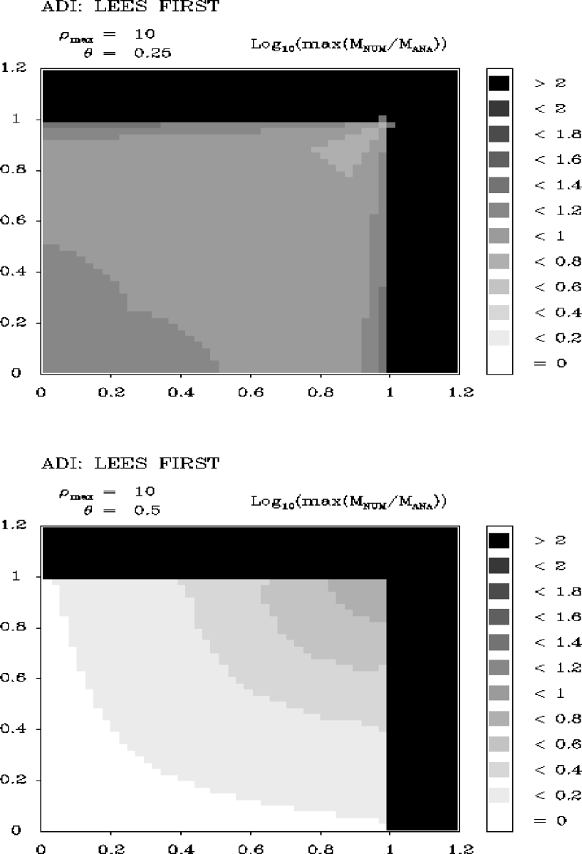
FIG. 13.: Stability for a method of Lees’ first type.

In the upper graph in Figure 13, we show the case where  $\theta\,=\,1/4$ . The finite difference scheme is unstable for at least some value of  $\rho$  at all values of the shift vector. This instability becomes much stronger whenever one of the components of the shift vector is greater than the speed of the waves. We recall that even in the one-dimensional case, the implicit scheme for $\theta=1/4$ is only conditionally stable, so the behavior here is no surprise. This figure also shows how the introduction of an operator splitting has broken the rotational symmetry of our problem: it is no longer the light-cone which is the important feature, but the rectangular region in which the light-cone is inscribed.

The lower graph corresponds to the case  $\theta\,=\,1/2$ , which is unconditionally stable in the one-dimensional case. In two dimensions, the scheme is still locally stable for values of the shift vector along the direction of the coordinate axis, just as the 1-D scheme was. However, instabilities appear for speeds in other directions. These instabilities are weak compared to those for speeds faster than the wave speed, but their presence will nevertheless be significant, as we will show in the examples of numerical integrations that we give below.

We have looked at larger values of the parameter  $\theta$ , but the situation doesn’t improve beyond $\theta=1/2$. Lees’ first scheme is therefore not very useful for grid speeds that are not aligned with the coordinate axis.

b Lees’ second scheme.

We next turn to Lees’ second method, for which the coefficients of the quadratic equation are:

$$A = \left\{1\,-\,i\rho\beta^{x}\>\sin\left(k_{x}\Delta x\right)\,-\,\rho^{2}\theta\,\left[g^{xx}-\left(\beta^{x}\right)^{2}\right]\>\left[\cos\left(k_{x}\Delta x\right)-1\right]\right\}$$ (IV.64)

$${}\times\left\{1\,-\,i\rho\beta^{y}\>\sin\left(k_{y}\Delta x\right)\,-\,\rho^{2}\theta\,\left[g^{yy}-\left(\beta^{y}\right)^{2}\right]\>\left[\cos\left(k_{y}\Delta x\right)-1\right]\right\},$$

$$B = -\,\left(2\rho^{2}\left(1-\theta\right)\left\{\left[g^{xx}-\left(\beta^{x}\right)^{2}\right]\left[\cos\left(k_{x}\Delta x\right)-1\right]+\,\left[g^{yy}-\left(\beta^{y}\right)^{2}\right]\left[\cos\left(k_{y}\Delta x\right)-1\right]\right\}\right.$$ (IV.71)

$$\quad{}\,-\,2\rho^{2}\,g^{xy}\>\sin\left(k_{x}\Delta x\right)\>\sin\left(k_{y}\Delta x\right)-\,i\rho^{2}\Delta x\,\left[\Gamma^{x}\>\sin\left(k_{x}\Delta x\right)\,+\,\Gamma^{y}\>\sin\left(k_{y}\Delta x\right)\right]$$

$$\quad{}+\,2i\rho^{3}\theta\,\left\{\beta^{x}\,\left[g^{yy}-\left(\beta^{y}\right)^{2}\right]\>\sin\left(k_{x}\Delta x\right)\>\left[\cos\left(k_{y}\Delta x\right)-1\right]\right.$$

$$\quad\qquad\left.{}+\,\beta^{y}\,\left[g^{xx}-\left(\beta^{x}\right)^{2}\right]\>\sin\left(k_{y}\Delta x\right)\>\left[\cos\left(k_{x}\Delta x\right)-1\right]\right\}$$

$$\quad{}+\,2\rho^{4}\theta^{2}\left[g^{xx}-\left(\beta^{x}\right)^{2}\right]\left[g^{yy}-\left(\beta^{y}\right)^{2}\right]\left[\cos\left(k_{x}\Delta x\right)-1\right]\left[\cos\left(k_{y}\Delta x\right)-1\right]$$

$$\quad{}\left.\,+\,2\rule[0.0pt]{0.0pt}{11.38109pt}\,\right),$$

$$C = -\,\left(\rho^{2}\theta\left\{\left[g^{xx}-\left(\beta^{x}\right)^{2}\right]\left[\cos\left(k_{x}\Delta x\right)-1\right]\,+\,\left[g^{yy}-\left(\beta^{y}\right)^{2}\right]\left[\cos\left(k_{y}\Delta x\right)-1\right]\right\}\right.$$ (IV.78)

$$\quad{}-\,i\rho\left[\beta^{x}\>\sin\left(k_{x}\Delta x\right)+\beta^{y}\>\sin\left(k_{y}\Delta x\right)\right]\,+\,\rho^{2}\beta^{x}\beta^{y}\>\sin\left(k_{x}\Delta x\right)\>\sin\left(k_{y}\Delta x\right)$$

$$\quad{}-\,i\rho^{3}\theta\left\{\beta^{x}\,\left[g^{yy}-\left(\beta^{y}\right)^{2}\right]\>\sin\left(k_{x}\Delta x\right)\>\left[\cos\left(k_{y}\Delta x\right)-1\right]\right.$$

$$\quad\qquad{}\left.+\,\beta^{y}\,\left[g^{xx}-\left(\beta^{x}\right)^{2}\right]\>\sin\left(k_{y}\Delta x\right)\>\left[\cos\left(k_{x}\Delta x\right)-1\right]\right\}$$

$$\quad{}-\,\rho^{4}\theta^{2}\left[g^{xx}-\left(\beta^{x}\right)^{2}\right]\left[g^{yy}-\left(\beta^{y}\right)^{2}\right]\left[\cos\left(k_{x}\Delta x\right)-1\right]\left[\cos\left(k_{y}\Delta x\right)-1\right]$$

$$\quad{}\left.\,-\,1\,\rule[0.0pt]{0.0pt}{11.38109pt}\right).$$

Again, these do not satisfy the boundedness condition Equation IV.50. In Figure 14 we again portray the cases for  $\theta\,=\,1/4$  and  $\theta\,=\,1/2$  . The situation is even worse than before: the instabilities in Lees’ second scheme grow faster than for the first scheme, and even for  $\theta>1/2$  there is only a very small region of stability just around the origin. Clearly, this scheme will not be practical for any moving grid.

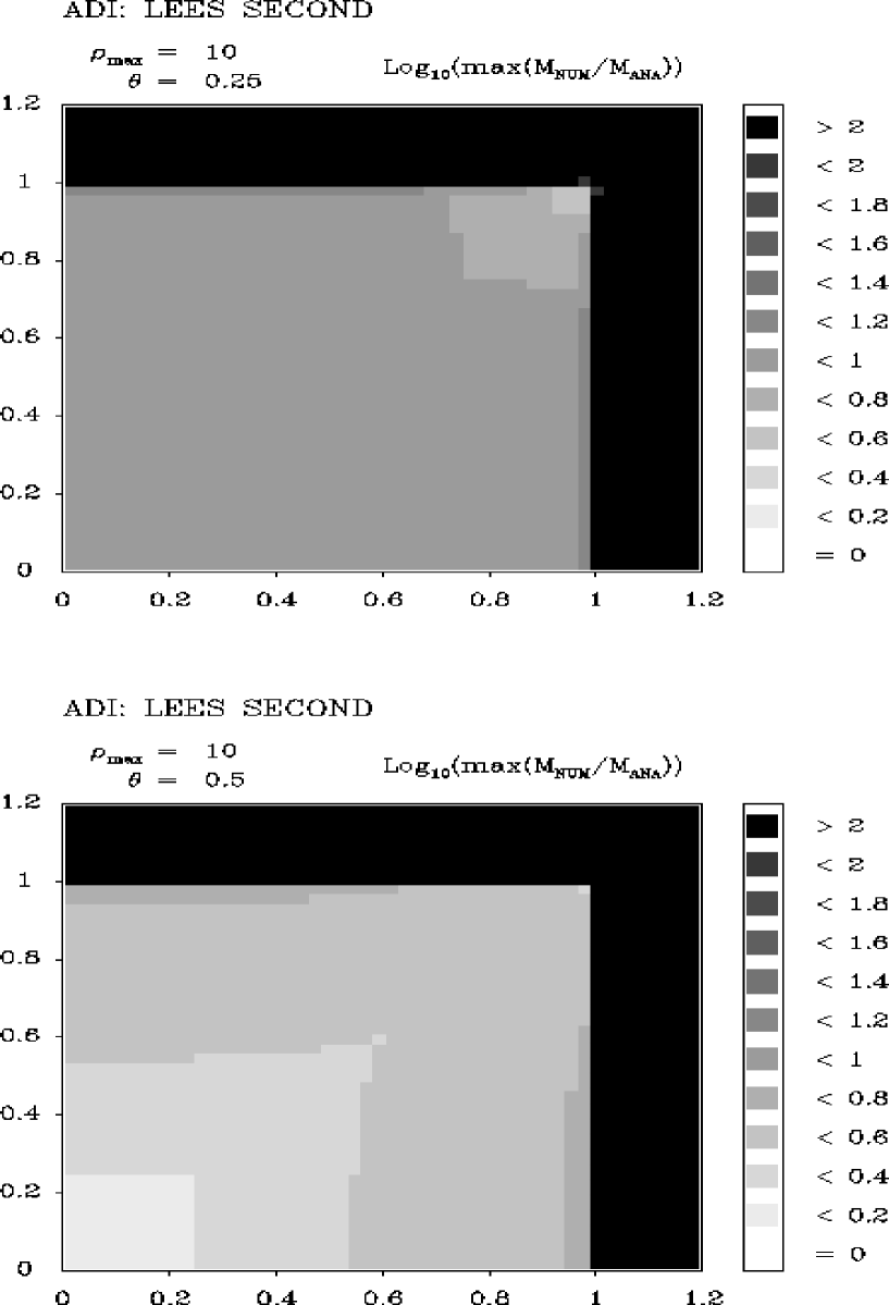
FIG. 14.: Stability for a method of Lees’ second type.

c The time-symmetric scheme.

We have found that both standard ADI methods become unstable when the reference frame is moving. Neither satisfies the symmetry condition Equation IV.50. Now we look in the same way at the time-symmetric scheme. The fact that this scheme does indeed satisfy Equation IV.50 can readily be seen from the form that the coefficients of the quadratic equation take in this case:

$$A = \left\{1\,-\,i\rho\beta^{x}\>\sin\left(k_{x}\Delta x\right)\,-\,\rho^{2}\theta\,\left[g^{xx}-\left(\beta^{x}\right)^{2}\right]\>\left[\cos\left(k_{x}\Delta x\right)-1\right]\right\}$$ (IV.80)

$$\quad{}\times\left\{1\,-\,i\rho\beta^{y}\>\sin\left(k_{y}\Delta x\right)\,-\,\rho^{2}\theta\,\left[g^{yy}-\left(\beta^{y}\right)^{2}\right]\>\left([\cos\left(k_{y}\Delta x\right)-1\right]\right\}\,,$$

$$B = -\,\left(2\rho^{2}\left(1-\theta\right)\left\{\left[g^{xx}-\left(\beta^{x}\right)^{2}\right]\left[\cos\left(k_{x}\Delta x\right)-1\right]+\left[g^{yy}-\left(\beta^{y}\right)^{2}\right]\left[\cos\left(k_{y}\Delta x\right)-1\right]\right\}\right.$$ (IV.86)

$$\quad{}\,-\,2\rho^{2}\,g^{xy}\>\sin\left(k_{x}\Delta x\right)\>\sin\left(k_{y}\Delta x\right)-\,i\rho^{2}\Delta x\,\left[\Gamma^{x}\>\sin\left(k_{x}\Delta x\right)\,+\,\Gamma^{y}\>\sin\left(k_{y}\Delta x\right)\right]$$

$$\quad{}+\,2\rho^{4}\theta^{2}\left[g^{xx}-\left(\beta^{x}\right)^{2}\right]\left[g^{yy}-\left(\beta^{y}\right)^{2}\right]\left[\cos\left(k_{x}\Delta x\right)-1\right]\left[\cos\left(k_{y}\Delta x\right)-1\right]$$

$$\quad\left.{}\,+\,2\rule[0.0pt]{0.0pt}{11.38109pt}\,\right)\,,$$

$$C = \left\{1\,+\,i\rho\beta^{x}\>\sin\left(k_{x}\Delta x\right)\,-\,\rho^{2}\theta\,\left[g^{xx}-\left(\beta^{x}\right)^{2}\right]\>\left[\cos\left(k_{x}\Delta x\right)-1\right]\right\}$$ (IV.89)

$$\quad{}\times\left\{1\,+\,i\rho\beta^{y}\>\sin\left(k_{y}\Delta x\right)\,-\,\rho^{2}\theta\,\left[g^{yy}-\left(\beta^{y}\right)^{2}\right]\>\left[\cos\left(k_{y}\Delta x\right)-1\right]\right\}\,.$$

Figure 15 shows the local stability analysis for this scheme, where again we show what happens for  $\theta\,=\,1/4$  and  $\theta\,=\,1/2$ .

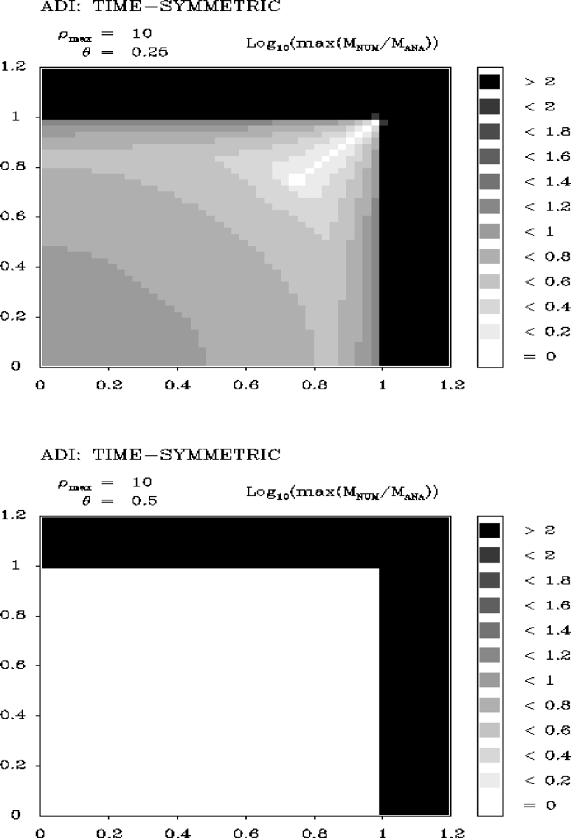
FIG. 15.: Stability for the time-symmetric scheme.

For the first case, the situation is no better than before: the scheme is unstable for practically every value of the shift vector. However, when we set $\theta=1/2$, the value that gave absolute stability in the one-dimensional case, the scheme becomes locally stable for every value of the shift vector inside the rectangular region that inscribes the light-cone. We find that this stability is maintained for larger values of  $\theta$  .

What we see here is effectively a ‘light-cone stability condition’, except for the fact that instead of a cone we now have a rectangle, as a consequence of the fact that the ADI splitting breaks the rotational symmetry of the problem. In the general case, this local stability condition can be expressed in the following way:

$$g^{i\,i}\,-\,\left(\beta^{i}\right)^{2}\,\geq\,0\qquad(\rm no\>\>sum)\,,$$ (IV.90)

where  $i$ may refer to any spatial direction.

The time-symmetric scheme has also the important property that in the stable region the numerical solutions will always be non-dissipative (at least in the non-accelerating case), that is:

$\displaystyle max\left(\frac{M_{\rm Num}}{M_{\rm Ana}}\right)\,=\,min\left(\frac{M_{\rm Num}}{M_{\rm Ana}}\right)\,=\,1$

This can be easily proved from the fact that this scheme satisfies condition IV.50: If the scheme has a dissipative solution with  $M_{\rm Num}\,<\,M_{\rm Ana}$ , then condition IV.50 together with the analytic boundedness condition (Equation IV.45) implies that it must also have an unstable solution with  $M_{\rm Num}\,>\,M_{\rm Ana}$ .

With the time-symmetric scheme we have then found what we are looking for: an absolutely locally stable, second-order accurate ADI decomposition for the finite difference approximation to the wave equation in a reference frame moving at any speed up to the wave speed in any direction. This scheme can be easily generalized to any number of spatial dimensions, as can be seen from its definition in the last section.

The restriction to frames moving slower than the wave speed is expected, of course. To remove it, we now define causal reconnection for the 2-dimensional case, using the time-symmetric ADI scheme as our starting point.

C Causal reconnection in 2 dimensions.

In the last section we found that the time-symmetric ADI scheme had stability properties superior to both the schemes of Less’ first and Lees’ second types. However, even for the time-symmetric scheme, instabilities appear as soon as one of the components of the grid speed becomes larger than the speed of the waves. In the one dimensional case, we saw that this instability could be avoided if we used a computational molecule based on the causal structure of the wave equation, and not in the motion of the individual grid points. We now want to generalize this approach to the two dimensional case.

We will again look for a computational molecule that guarantees that the light-cone is properly represented in the immediate vicinity of the central point. For the moment we will assume that we have already found the points that form such a molecule. We then introduce the local coordinate system  $\{\left.x^{i}\right.^{\prime},t^{\prime}\}$  adapted to the causal molecule as a direct generalization of the one dimensional case:

$$\left.\begin{array}[]{ll}\left.x^{i}\right.^{\prime}\,:=\,\left(x^{i}-x^{i}_{t_{0}}\right)-P^{i}\left(t\right)\,,\\ \\ t^{\prime}\>\>\>\,:=\,t\,,\end{array}\right\}$$ (IV.91)

where  $\{x^{i}_{t_{0}},t_{0}\}$  are the coordinates of the central point of the molecule, and where

$$P^{i}\left(t\right) = A^{i}\,\frac{\left(t-t_{0}\right)^{2}}{2}+B^{i}\,\left(t-t_{0}\right)+x^{i}_{0}\>,$$ (IV.92)

$$A^{i} := \left(\frac{x^{i}_{t_{0}+\Delta t}-2x^{i}_{t_{0}}+x^{i}_{t_{0}-\Delta t}}{\left(\Delta t\right)^{2}}\right)\rule[0.0pt]{0.0pt}{22.76219pt}\,,$$ (IV.93)

$$B^{i} := \left(\frac{x^{i}_{t_{0}+\Delta t}-x^{i}_{t_{0}-\Delta t}}{2\,\Delta t}\right)\,.$$ (IV.94)

In the new coordinate system, the wave equation has the same form as before, except for the substitutions:

$$\beta^{i}\,\longrightarrow\,\beta^{i}+\frac{A^{i}\,\left(t-t_{0}\right)+B^{i}}{c}\,,\hskip 56.9055pt\Gamma^{i}\,\longrightarrow\,\Gamma^{i}-\frac{A^{i}}{c^{2}}\,.$$ (IV.95)

Since in the finite difference approximation the coefficients should be evaluated at the center of the molecule, the above expressions will reduce to:

$$\beta^{i}\,\longrightarrow\,\beta^{i}+\frac{B^{i}}{c}\,,\hskip 56.9055pt\Gamma^{i}\,\longrightarrow\,\Gamma^{i}-\frac{A^{i}}{c^{2}}\,.$$ (IV.96)

We know that the original finite difference approximation was locally stable as long as Equation IV.90 was satisfied. This implies that the approach based on the reconnected molecule will be stable if

$$g^{i\,i}-\left(\beta^{i}+\frac{B^{i}}{c}\right)^{2}\,\geq\,0\hskip 56.9055pt\forall i\,.$$ (IV.97)

As in the one-dimensional case, we will say that the given three points form a proper causal molecule if the last condition is satisfied.

We will now define a generalization to two dimensions of the concept of effective numerical light-cone. We do this by defining first the axis of this numerical light-cone as the line:

$$x^{i}_{a}\left(t\right)\,:=\,x^{i}_{t_{0}}\,-\,\beta^{i}c\,\left(t-t_{0}\right)\,+\,\frac{1}{2}\,\Gamma^{i}c^{2}\left(t-t_{0}\right)^{2}\,.$$ (IV.98)

The numerical light-cone will then be defined by taking at each time the region covered by a rectangle that is centered at the axis and has sides:

$$2c\,\Delta t\,\left(g^{i\,i}\right)^{1/2}\,.$$ (IV.99)

With this definition, the numerical “light-cone” is really a prism and not a cone. It is not difficult to prove now that if the points  $x^{i}_{t_{0}-\Delta t}$  and  $x^{i}_{t_{0}+\Delta t}$  are inside the numerical light-cone of  $x^{i}_{t_{0}}$ , then we will have:

$$\left(\beta^{i}+\frac{B^{i}}{c}\right) \in \left[-\left(g^{i\,i}\right)^{1/2}\,,\,\left(g^{i\,i}\right)^{1/2}\,\,\rule[-2.84526pt]{0.0pt}{19.91692pt}\right]\,,$$ (IV.100)

$$\left(\Gamma^{i}-\frac{A^{i}}{c^{2}}\right) \in \left[-\frac{2\left(g^{i\,i}\right)^{1/2}}{\left(c\Delta t\right)}\,,\,\frac{2\left(g^{i\,i}\right)^{1/2}}{\left(c\Delta t\right)}\,\right]\,.$$ (IV.101)

This means that the three points do form a proper causal molecule, and also that the acceleration in the new local coordinates will be bounded.

As in the one-dimensional case, we can guarantee that proper causal molecules can be formed everywhere if we ask for two conditions:

1. Every parent has at least two children. There must always be at least one grid point in the upper and lower time levels inside the numerical light-cones of all points in the middle time level. It is easy to see that this will require:

   $$2\,\rho\,\min\left(g^{i\,i}\right)^{1/2}\,\geq\,1\hskip 56.9055pt\forall i\,.$$ (IV.102)

2. Every child has a parent. All the grid points in the upper and lower time levels must be inside the numerical light-cone of at least one point in the middle time level. We guarantee this by asking that the light-cones of the points in the middle time level should cover completely the upper and lower time levels, in other words that the union of the intersections of these light-cones with both the upper and lower levels should be the entire grid.

   Let us consider a square of nearest neighbours in the middle time level. We want their numerical light-cones to cover the whole quadrilateral area defined by the points where the axis of those light-cones intersect the adjacent time levels. A sufficient condition for this to happen is to ask for the sides of this quadrilateral to be smaller than the spread of the smallest light-cone divided by  $\sqrt{2}$  (this factor arises from the fact that the diagonals of a square are  $\sqrt{2}$  times larger than its sides).

   Following now the same procedure as before, we can show that this condition takes the form:

   $$\frac{2}{\sqrt{2}}\,\,\rho\,\min\left(g^{i\,i}\right)^{1/2} \geq \left\{1\,+\,2\,\max\left(d_{11},d_{22}\right)\,+\,\left[\max\left(d_{11},d_{12}\right)\rule[0.0pt]{0.0pt}{14.22636pt}\right]^{2}\right.$$ (IV.104)

   $$\left.+\,\left[\max\left(d_{21},d_{22}\right)\rule[0.0pt]{0.0pt}{14.22636pt}\right]^{2}\right\}^{1/2}\hskip 56.9055pt\forall i\,.$$

   where the quantities  $d_{jk}$  are defined as:

   $$d_{jk}\,=\,\rho\,\left(\,\Delta x\,\left|\frac{\partial\beta^{j}}{\partial x^{k}}\right|\,+\,\frac{\left(\Delta x\right)^{2}}{2}\,\left|\frac{\partial^{2}\beta^{j}}{\partial x^{1}\,\partial x^{2}}\right|\>\right)\,+\,\rho^{2}\,\frac{\left(\Delta x\right)^{2}}{2}\,\left(\frac{\partial\Gamma^{j}}{\partial x^{k}}\right)$$ (IV.105)

   and the maximum should be taken over all values of  $x^{i}$ . As in the one-dimensional case, the last condition is valid only to second order in  $\Delta x$ .

Conditions IV.102 and IV.104 are the causal reconnection conditions in the two dimensional case. They will guarantee that proper causal molecules can always be formed.

D Numerical examples.

To test the finite difference methods that we have developed, we will consider two different situations: a grid moving with a uniform speed, and a grid rotating with constant angular velocity.

1 Uniformly moving grid.

We will first study the case of the grid moving with uniform speed, in order to show the advantages of the time-symmetric scheme. If the grid is moving with velocity  $\vec{v}\,=\,\left(v^{x},v^{y}\right)$ , it is not difficult to see that:

$$g_{i\,j} = \delta_{i\,j}$$ (IV.106)

$$\beta^{i} = v^{i}/c,\quad\mbox{and}$$ (IV.107)

$$\Gamma^{x} = \Gamma^{y}\,=\,0\,.$$ (IV.108)

Using these values for the coefficients, we have studied the numerical solution to the wave equation for a number of examples, comparing the three different ADI methods developed earlier. The first set of graphs (Figure 16) show the result of one such calculation for a scheme of Lees’ first type. In the graphs we show the grid region  $[(0,10)\times(0,10)]$ , and we calculate the evolution of a Gaussian wave packet originally at rest at the point  $(7,7)$ . For simplicity, we have imposed reflecting boundaries. We have taken a time-step such that $\rho=1$, which means that we are well beyond the Courant limit. The evolution is followed using a grid with a speed given by:

$\displaystyle\vec{v}\,=\,(\frac{1}{2}\,,\frac{1}{2}\,),\qquad|\vec{v}|=0.707<1,$

where we have taken  $c\,=\,1$ .

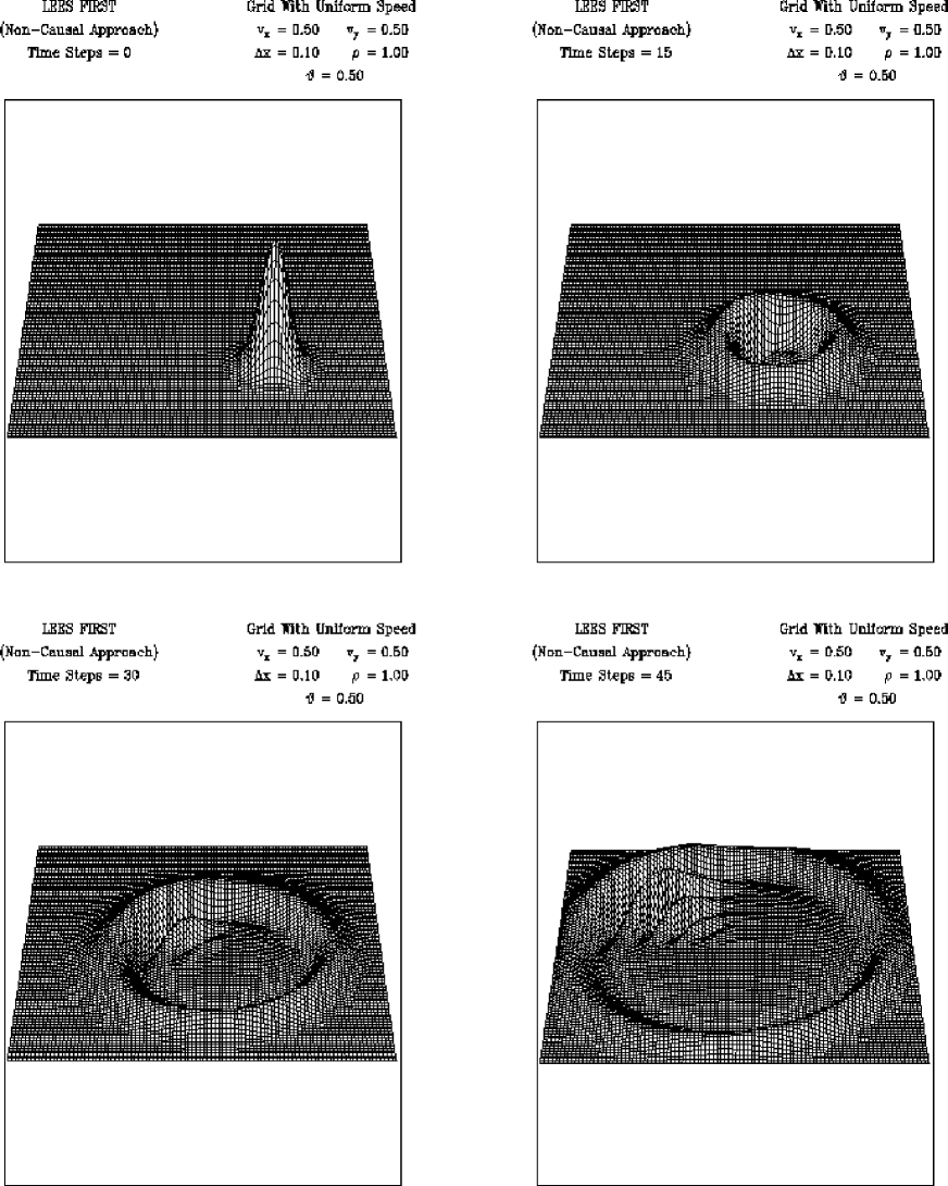
FIG. 16.: Uniform shift vector: Lees’ first scheme.

We see how an instability is beginning to grow even though the grid is moving slower than the wave speed. This is precisely in accordance with the results of our local stability analysis. This instability grows slowly, as expected. Nevertheless, it is clear that its presence is unacceptable in a calculation of any duration. If we use a method of Lee’s second type, the instability takes longer to develop, but once it appears it grows very fast, much faster that with Lees’ first method. The fact that the instabilities in general take longer to appear with Lees’ second method can be traced to the particular wave modes that are involved. As we can see in the graphs, the instabilities in Lees’ first method are associated with relatively long wavelengths (several grid points), and since these modes are already present in the initial data, they start growing right away. In Lees’ second method, however, the instabilities turn out to be associated with very short wavelengths (one or two grid points), which do not contribute significantly to the initial data. These means that, even though the instabilities are more violent with this method, it will take a long time for the unstable modes to grow to the scale of the real solution.

In the next set of graphs (Figure 17) we have applied the time-symmetric scheme to the same problem. The instability has completely disappeared. This is again in agreement with our previous conclusions, and shows the superiority of this method.

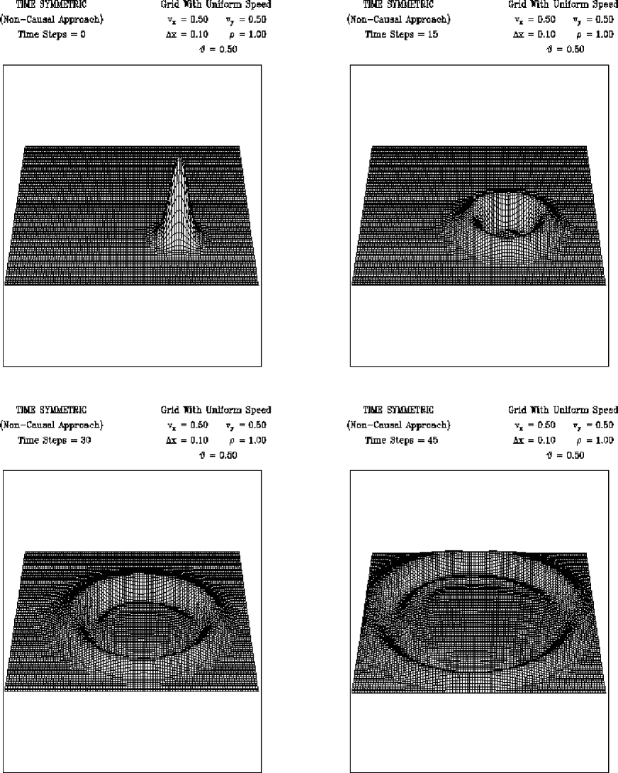
FIG. 17.: Uniform shift vector: time-symmetric scheme.

We have performed similar calculations for many different values of the grid speed and we have found the essentially similar results. The time-symmetric scheme remains stable as long as the grid moves slower than the waves, while the other schemes present instabilities for quite small grid velocities.

2 Rotating grid.

In order to show the advantage of causal reconnection of the computational molecules when the grid moves very fast, we will consider now an example with a grid rotating with the constant angular velocity  $\omega$  . It is not difficult to show that:

$$g_{i\,j} = \delta_{i\,j}$$ (IV.109)

$$\beta^{x}\,=\,-\frac{\omega}{c}\,y\,, \beta^{y}\,=\,\frac{\omega}{c}\,x\,,$$ (IV.110)

$$\Gamma^{x}\,=\,-\frac{\omega^{2}}{c^{2}}\,x\,, \Gamma^{y}\,=\,-\frac{\omega^{2}}{c^{2}}\,y\,.$$ (IV.111)

To test for local stability when using causal reconnection, we take

$\displaystyle\omega\,=\,0.25\,$

in units in which $c=1$ and the grid extends over the range  $[(-5,5)\times(-5,5)]$ . This means that the centers of the edges of the grid will be moving faster than the wave speed, with a linear velocity of $1.25$, while the corners will be going even faster.

The next graphs show the results of a time-symmetric calculation, first using a “direct” calculation (fixed computational molecule) and second using causal reconnection. Again we use a time-step such that $\rho=1$. In Figure 18, we show the evolution of a Gaussian wave packet originally at rest at the center of the grid, using the direct approach. We see how after  $32$  time-steps an instability has appeared close to the boundaries. Only five time-steps later, this instability has grown so large that the original wave is no longer visible (the scale is automatically adjusted to display the largest value of the function).

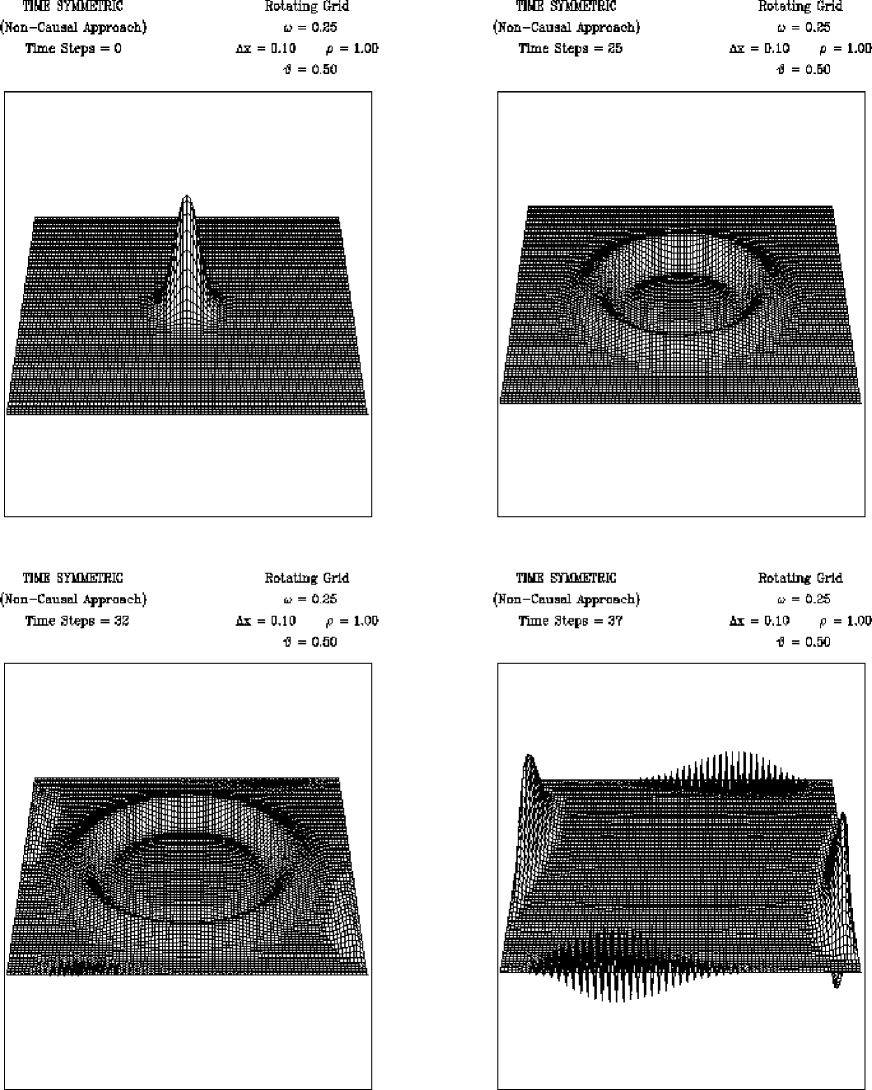
FIG. 18.: Rotating grid: non-causal approach.

Figure 19 shows the same calculation using causal reconnection. The instability is not present. In fact, we have done the same calculation with much larger values of the angular velocity (up to  $\omega\,=\,3.0$ , where the edge is travelling at 15 times the wave speed), and the scheme remains locally stable.

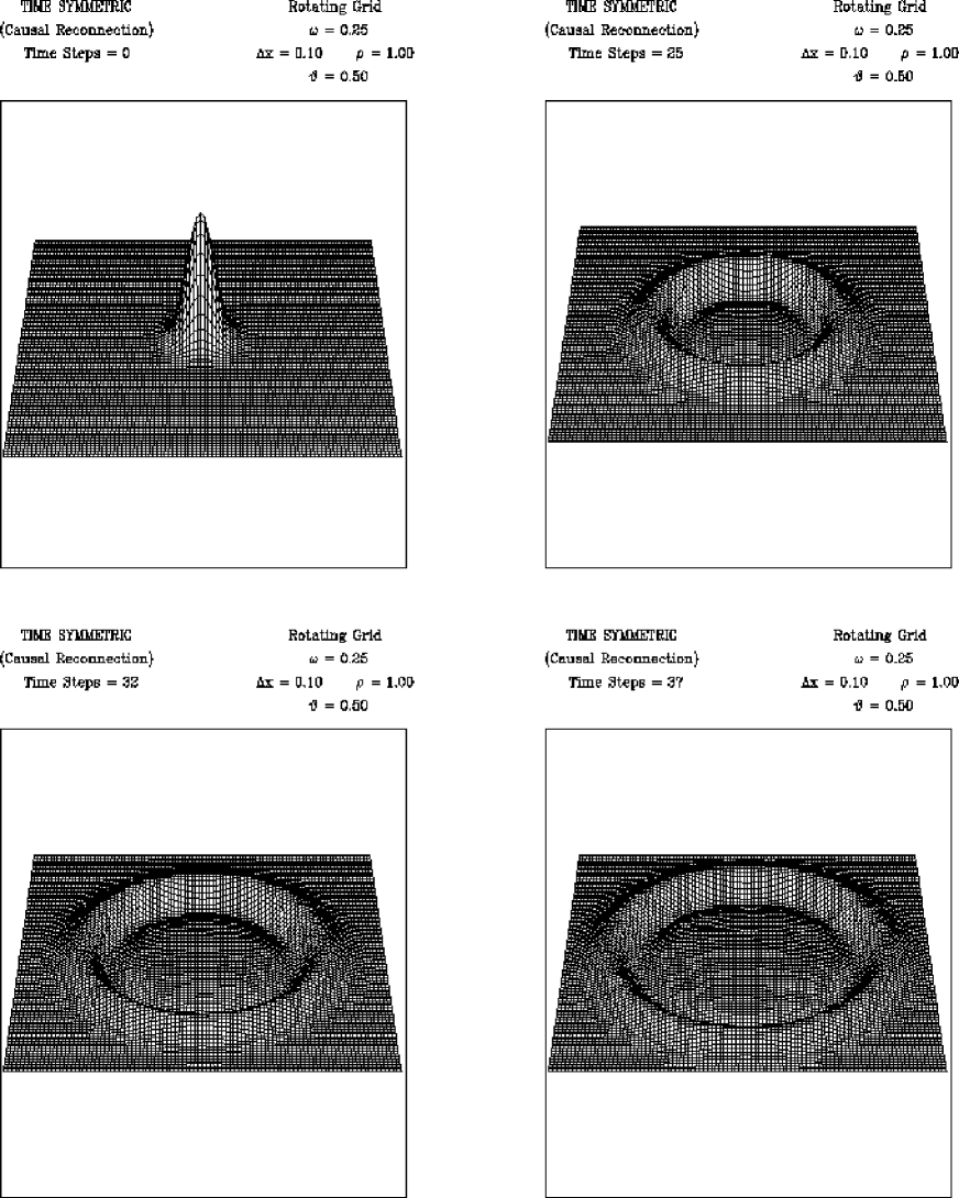
FIG. 19.: Rotating grid: causal reconnection.

These examples demonstrate dramatically that time-symmetric ADI can be married with causal reconnection, and that together the two techniques provide a robust difference approximation to the wave equation on a moving grid. These methods are stable, offer all the computational advantages of ADI schemes, and remain second order accurate in  $\Delta x$  and  $\Delta t$ .

A comment on how to enforce causal reconnection at the boundaries seems in order here. In all our examples we have taken the practical approach of setting the value of the wave function to zero whenever a complete causal molecule cannot be formed. This can happen not only at the boundaries, but also at inner points close to the boundaries for large enough grid speeds. The philosophy behind this approach is simple: If the causal molecule is incomplete, then we would need information from outside the grid to evolve the wave function at that place. If we impose the condition that no information can come from the outside, then we must take the value of the wave function as zero at that point. This requirement can be relaxed somewhat be using an outgoing wave boundary condition whenever we can still find a causally related point in the previous time level, but not before that. At places where one can’t even find a causally related point in the previous time level, the only legitimate thing one can do is to set the value of the wave function to zero.

V Conclusions.

The wave equation we have studied here is a prototype for more complex equations of mathematical physics, such as the Einstein field equations. In fact, many hyperbolic systems in mathematical physics can be formulated in terms of the wave operator. One would expect the instabilities we have found here to be generic: any numerical approximation to a hyperbolic system on a shifting grid should exhibit them.

Only experience will show us just how well our cures for these generic instabilities transfer to more interesting equations. However, the instabilities we have described here are cured by the application of two clear physical principles, causality and time-reflection invariance. It seems clear that it would be asking for trouble not to incorporate these principles into the design of algorithms for the numerical integration of any fundamental physical equations.

We have, of course, studied in detail only one second-order differential equation in one and two dimensions. The restriction to two dimensions is not important. The physical principles involved do not depend on the number of dimensions, and the savings obtained by using an ADI scheme instead of a fully-implicit formulation increase rapidly with the number of dimensions. In many physical systems, it is advantageous to formulate the equations of the theory as first-order differential equations. This is true in hydrodynamics and in many studies of general relativity. The general principles of causality and time-reflection invariance extend in a simple way to such systems. Time-symmetric ADI should prove relatively straightforward to apply to more complicated systems of equations, provided the original differential equations embody time symmetry.

Causality may be less straightforward in nonlinear equations, where the structure of the characteristic cone will depend on the solution, and so the exact causal relationships between time-levels cannot be decided independently of solving the equations. However, causal reconnection is implemented via an inequality: one requires that grid points should be within the characteristic cones of their relatives at the previous time-step. In most cases, one would hope that the inequality can be assured simply by extrapolation from the behavior of the characteristic cones on the known time-steps.

An important area for the application of the techniques we have developed here would be numerical fluid dynamics, where the study of wave phenomena in supersonic flows is a natural place to expect causality problems, and where the interest in three-dimensional problems makes ADI essential in many cases.

In some restricted situations, it may be straightforward to apply these techniques; for example, a neutron star moving supersonically through a grid in general relativity will, if treated in the standard way, use acausal computational molecules. Using causal reconnection, adapted to the characteristics of the fluid problem, should prevent instabilities of the type we have found here.

But the application of our techniques to more general problems in fluid dynamics will not be automatic. Causal reconnection will have to be generalized to deal with hydrodynamic shocks. At a shock, the regular causal structure of the fluid breaks down. This does not mean that causal reconnection cannot be implemented there. On the contrary, the fact that a causal algorithm is constantly mapping the structure of the characteristics means that it can be programmed automatically to locate and to identify shocks.

The idea of correctly representing the causal structure of the original differential equation is not new, existing methods for handling shocks and related transport problems, such as upwind differencing [9] and Godunov methods [10], are already based on the local structure of the characteristics of the fluid. These ideas have also been introduced in the numerical study of steady supersonic flows, where the direction of flow behaves like a time coordinate and the equations become hyperbolic. Integration methods have been developed that use retarded differences in the upstream direction to maintain stability [11], [12]. All these methods differ from causal reconnection in the fact that they keep using only the nearest neighbours to build the computational molecules. We have recently become aware, however, of a paper by E. Seidel and Wai-Mo Suen that introduces an idea they call “causal differencing”, that is very similar to our causal reconnection [13].

Fluid dynamics also presents special challenges to time-symmetric ADI. The usual equations of inviscid gas dynamics are time-symmetric, but the presence of viscosity or shocks introduces a fundamental irreversibility into the problem. We hope to treat the fluid dynamic problem in a future paper.

We are confident, however, that the present techniques will generalize easily to problems in numerical general relativity, such as that of the motion of black holes through fixed grids. Causal reconnection should allow the equations to remain stable and causal. Moreover, the computational advantages offered by ADI schemes, of permitting stable large time-steps (provided the physical situation allows such steps to remain accurate) while avoiding time-consuming sparse-matrix solutions, can be obtained without sacrificing accuracy or stability. It is hard now to imagine any situation in numerical integrations of the vacuum field equations of general relativity where one would use implicit methods without employing time-symmetric ADI.

Appendix A. Derivation of Wave Equation on a Shifting Grid.

In this appendix we will sketch the derivation of Equation II.3 by making use of elegant tensorial techniques. There are many alternative approaches, of course, and a reader unfamiliar with tensors can obtain the same result in a straightforward, but rather long, way simply by making the following general change of variables in the original wave equation from the physical (inertial) coordinates $\{\xi^{\mu}\}$ to the computational coordinates $\{x^{\alpha}\}$:

$$x^{i}\,=\,x^{i}(\xi^{\mu})\,,\qquad x^{0}\,=\,\xi^{0}\,,$$ (A.1)

with the associated change of derivatives

$$\frac{\partial}{\partial\xi^{i}}\,=\,\frac{\partial x^{k}}{\partial\xi^{i}}\,\frac{\partial}{\partial x^{k}}\,,\qquad\frac{\partial}{\partial\xi^{0}}\,=\,\frac{\partial x^{k}}{\partial\xi^{0}}\,\frac{\partial}{\partial x^{k}}\,+\,\frac{\partial}{\partial x^{0}}\,.$$ (A.2)

The functions that we have identified as the shift vector  $\beta^{i}$ , the spatial metric  $g_{\,i\,j}$  and the  $\Gamma^{i}$  coefficients in Equations (II.4), (II.5) and (II.8) come out as part of the algebra. A reader who wants an introduction to the use of tensors in mathematical physics is invited to consult reference [14].

We will start from the expression of the wave equation in a general coordinate system:

$$\Box^{2}\,\phi\,=\,(\gamma^{\mu\nu}\,\phi_{;\,\mu})_{;\,\nu}\,=\,0\,,$$ (A.3)

where the semicolon stands for covariant derivative. Using the explicit expression for the covariant derivatives, the last equation takes the form:

$$\gamma^{\mu\nu}\,\frac{\partial^{2}\phi}{\partial x^{\mu}\,\partial x^{\nu}}-\Gamma^{\lambda}\,\frac{\partial\phi}{\partial x^{\lambda}}=0\,,$$ (A.4)

where the coefficients  $\Gamma^{\lambda}$  are defined in terms of the Christoffel symbols as:

$$\Gamma^{\lambda}\,:=\,\gamma^{\mu\nu}\,\Gamma^{\lambda}_{\mu\nu}\,.$$ (A.5)

Our first task is, then, to find the inverse metric $\gamma^{\mu\nu}$. The metric in the new coordinates is given by

$$\gamma_{\mu\nu}\,=\,\frac{\partial\xi^{\alpha}}{\partial x^{\mu}}\frac{\partial\xi^{\beta}}{\partial x^{\nu}}\>\>\eta_{\alpha\beta}\,,$$ (A.6)

with $\eta_{\alpha\beta}$ the Minkowski metric tensor:

$$\left.\begin{array}[]{lll}\eta_{00}\>=\,-1\,,\\ \eta_{\,i\,i}\>=\,\>\>1\,\hskip 34.1433pt({\rm no\hskip 5.69054ptsum})\,,\\ \eta_{\mu\nu}\,=\,\>\>0\hskip 42.67912pt\mu\,\neq\,\nu\,.\end{array}\right\}$$ (A.7)

We now note that for a line of constant  $\{\xi^{i}\}$  we have

$\displaystyle 0=\left.\frac{d\xi^{i}}{dt}\right|_{\{\xi^{i}\}}=\,\frac{\partial\xi^{i}}{\partial x^{j}}\left.\frac{dx^{j}}{dt}\right|_{\{\xi^{i}\}}+\frac{\partial\xi^{i}}{\partial t}\,,$

which implies

$$\frac{\partial\xi^{i}}{\partial t}\,=\,-\frac{\partial\xi^{i}}{\partial x^{j}}\left.\frac{dx^{j}}{dt}\right|_{\{\xi^{i}\}}\,.$$ (A.8)

Using now the definition of the shift vector (Equation II.4) and writing  $x^{0}\,=\,ct$  we find:

$$\frac{\partial\xi^{i}}{\partial x^{0}}\,=\,\beta^{j}\,\frac{\partial\xi^{i}}{\partial x^{j}}\,.$$ (A.9)

This is an important relation, and we will use it to rewrite the metric coefficients given by Equation A.6.

For the mixed components in space and time of  $\gamma_{\mu\nu}$  we find:

$$\gamma_{\,0\,i}\,=\,\gamma_{\,i\,0} = \sum_{l=1}^{n}\,\frac{\partial\xi^{l}}{\partial x^{i}}\,\frac{\partial\xi^{l}}{\partial x^{0}}$$

$$= \,\beta^{j}\,\sum_{l=1}^{n}\,\frac{\partial\xi^{l}}{\partial x^{i}}\,\frac{\partial\xi^{l}}{\partial x^{j}}\,,$$

and finally:

$$\gamma_{0\,i}\,=\,\gamma_{\,i\,0}\,=\,\gamma_{\,i\,j}\,\beta^{j}\,=\,g_{\,i\,j}\,\beta^{j}\,.$$ (A.10)

In a similar way we can find the coefficient  $\gamma_{00}$ :

$$\gamma_{00}\, = \,-\left(\frac{\partial\xi^{0}}{\partial x^{0}}\right)^{2}+\sum_{l=1}^{n}\,\left(\frac{\partial\xi^{l}}{\partial x^{0}}\right)^{2}$$

$$= \,-1+\sum_{l=1}^{n}\,\beta^{j}\,\frac{\partial\xi^{l}}{\partial x^{j}}\,\beta^{i}\,\frac{\partial\xi^{l}}{\partial x^{i}}\,,$$

and from this we obtain:

$$\gamma_{00}\,=\,-1+g_{\,i\,j}\,\beta^{i}\beta^{j}\,.$$ (A.11)

We will adopt the convention that the indices of the shift vector can be raised and lowered by using only the spatial metric:

$$\beta_{\,i}\,=\,g_{\,i\,j}\,\beta^{j}\,,\hskip 28.45274pt\beta^{i}\,=\,g^{i\,j}\,\beta_{\,j}\,,$$ (A.12)

where  $g^{i\,j}$  are the coefficients of the inverse of the spatial metric matrix  $g_{\,i\,j}$ .

The coefficients of  $\gamma_{\mu\nu}$  can now be written as:

$$\gamma_{\mu\nu}\,=\,\left(\begin{array}[]{rr}(-1+\beta_{i}\beta^{i})&\beta_{k}\\ \vspace{2mm}\hfil\\ \beta_{j}&g_{j\,k}\end{array}\right)\,.$$ (A.13)

Using the last expression it is not difficult to see that the coefficients of the inverse metric  $\gamma^{\mu\nu}$  will be given by:

$$\gamma^{\mu\nu}\,=\,\left(\begin{array}[]{ll}-1&\hskip 25.60747pt\beta^{k}\\ \vspace{2mm}\\ \>\>\beta^{j}&(g^{j\,k}-\beta^{j}\beta^{k})\end{array}\right)\,.$$ (A.14)

Having found  $\gamma^{\mu\nu}$, we will now look for an expression for the coefficients  $\Gamma^{i}$ . Since the original coordinates $\{\xi^{\alpha}\}$ define an inertial reference frame, the Christoffel symbols can be expressed in terms of their transformation to the general coordinates:

$$\Gamma^{\lambda}_{\mu\nu}\,=\,\frac{\partial x^{\lambda}}{\partial\xi^{\alpha}}\,\frac{\partial^{2}\xi^{\alpha}}{\partial x^{\mu}\,\partial x^{\nu}}\,.$$ (A.15)

From the last expression it is easy to see that:

$$\Gamma^{0}_{\mu\nu}\,=\,0\,,$$ (A.16)

which in turn means:

$$\Gamma^{0}\,=\,0\,.$$ (A.17)

On the other hand, from the general expression for the Christoffel symbols:

$$\Gamma^{\lambda}_{\mu\nu}\,:=\,\frac{1}{2}\,\gamma^{\lambda\alpha}\left[\frac{\partial\gamma_{\mu\alpha}}{\partial x^{\nu}}\,+\,\frac{\partial\gamma_{\nu\alpha}}{\partial x^{\mu}}\,-\,\frac{\partial\gamma_{\mu\nu}}{\partial x^{\alpha}}\right]\,,$$ (A.18)

it is not difficult to show that:

$$\Gamma^{i}\,:=\,\gamma^{\mu\nu}\,\Gamma^{i}_{\mu\nu}\,=\,-\frac{1}{\sqrt{g}}\left\{\frac{\partial}{\partial t}\left(\sqrt{g}\beta^{i}\right)+\frac{\partial}{\partial x^{j}}\left[\sqrt{g}\left(g^{ij}-\beta^{i}\beta^{j}\right)\right]\right\}.$$ (A.19)

Using the previous results, we can finally rewrite Equation A.4 in the following way:

$$(g^{i\,k}-\beta^{i}\beta^{k})\,\frac{\partial^{2}\phi}{\partial x^{i}\,\partial x^{k}}+\frac{2\beta^{i}}{c}\,\frac{\partial^{2}\phi}{\partial x^{i}\,\partial t}-\Gamma^{i}\,\frac{\partial\phi}{\partial x^{i}}-\frac{1}{c^{2}}\,\frac{\partial^{2}\phi}{\partial t^{2}}\,=\,0\,.$$ (A.20)

This is the final form of the wave equation in the coordinate system adapted to the motion of the grid.

Appendix B. Implementation of Causal Reconnection.

In this appendix, we discuss one algorithm that determines the positions of the points that form the causal computational molecules. We will consider the case of an arbitrary number of spatial dimensions  $n$ . The particular cases of one and two dimensions can then be found in a straightforward way.

There are many different ways of finding the closest causally connected grid points. For example, if it is possible to find the transformation of coordinates that takes us back to the original inertial reference frame

$$\xi^{i}\,=\,\xi^{i}\left(x^{j},t\right)\,,$$ (B.1)

then we could use the fact that in that reference frame the causal structure is particularly simple: we would simply select those points in the different time levels that have the closest values of  $\left\{\xi^{i}\right\}$ . This method, however, will only be useful in a few special cases. Indeed, in the general case it may prove almost impossible to find the functional relation (B.1).

With this in mind, we have developed a method that can be applied in the general case. Let us then assume that we are given a point in the last time level  $\left\{t_{0}+\Delta t\right\}$  with position  $x^{i}_{t_{0}+\Delta t}$ . Our aim is to find points  $x^{i}_{t_{0}}$  and  $x^{i}_{t_{0}-\Delta t}$  in the two previous time levels in such a way as to guarantee that a proper causal molecule will be formed. We have already seen that this will happen if both  $x^{i}_{t_{0}-\Delta t}$  and  $x^{i}_{t_{0}+\Delta t}$  are inside the numerical light-cone of  $x^{i}_{t_{0}}$ .

Our algorithm to find the proper causal molecules linking the grids at time-steps  $t_{0}+\Delta t$,  $t_{0}$, and  $t_{0}-\Delta t$ assumes that the causal reconnection condition holds. (If it doesn’t, then remedial action, changing $\Delta t$ or $\Delta x^{i}$, is required.) Our procedure is the following.

1. Choose some point  $x^{i}_{t_{0}+\Delta t}$ . The center of its causal molecule will be that grid point  $y^{i}_{t_{0}}$  for which the following function reaches a minimum:

   $$f_{1}\left(y^{i}\right)\,:=\,\sum_{i=1}^{N}\left\{\left[y^{i}\,-\,\beta^{i}\left(y^{j},t_{0}\right)\Delta t\,+\,\frac{1}{2}\,\Gamma^{i}\left(y^{j},t_{0}\right)\left(\Delta t\right)^{2}\right]-x^{i}_{t_{0}+\Delta t}\,\right\}^{2}\,.$$ (B.2)

   This minimum can easily be found by standard multi-dimensional search techniques. Once the minimum is found, we have our best approximation to the exact inverse coordinate transformation: the point $x^{i}$ is approximately at the same spatial location as $y^{i}$ in the original inertial frame.

2. Once we have found the appropriate  $y^{i}_{t_{0}}$ , we look in the third time level  $\left\{t_{0}-\Delta t\right\}$  for the completion of the causal molecule, the point  $z^{i}_{t_{0}-\Delta t}$  that minimizes the function:

   $$f_{2}\left(z^{i}\right)\,:=\,\sum_{i=1}^{N}\left\{\left[y^{i}_{t_{0}}\,+\,\beta^{i}\left(y^{j}_{t_{0}},t\right)\Delta t\,+\,\frac{1}{2}\,\Gamma^{i}\left(y^{j}_{t_{0}},t\right)\left(\Delta t\right)^{2}\right]-z^{i}\,\right\}^{2}\,.$$ (B.3)

   This is much easier than the previous step because we already have the point  $y^{i}_{t_{0}}$ , so we don’t have to calculate again the functions  $\beta$  and  $\Gamma$ . In fact, minimizing  $f_{2}$  is equivalent to finding the point  $z^{i}$  in the third time level that is closest to the axis of the light cone of  $y^{i}_{t_{0}}$  in the original inertial frame. We do not have to go through the grid again to find this point.

3. So far we have constructed only one molecule. One needs to repeat the above steps for all points at time-step $t_{0}+\Delta t$, but of course the best guess for a causal molecule for any grid point is simply to translate the molecule found for its neighbor. This will occasionally fail, but only by one grid point. So the minimization steps will require a computing effort that is only proportional to the number of grid points.

It is not difficult to prove that, whenever the causal reconnection conditions hold, this algorithm does indeed produce a proper causal molecule. For reasons indicated above, the computational effort is proportional to the number of grid points. In complex problems, such as general relativity, this is likely to be a very small overhead.

REFERENCES

- [1] C.W. Misner, K.S. Thorne and J.A. Wheeler, Gravitation, W.H. Freeman and Co., U.S.A., 1973.
- [2] J.W. York, ‘Kinematics and Dynamics of General Relativity’ in: Sources of Gravitational Radiation, ed. L.L. Smarr, pp. 83-126, Cambridge University Press, U.S.A., 1979.
- [3] W.H. Press, B.P. Flannery, S.A. Teukolsky and W.T. Vetterling, Numerical recipes: The Art of Scientific Computing, Cambridge University Press, U.S.A., 1989.
- [4] R.D. Richtmyer and K.W. Morton, Difference Methods for Initial-Value Problems, 2nd. ed., Interscience, U.S.A, 1967.
- [5] G. Strang, SIAM J. Num. Anal., 5, p. 506 (1968).
- [6] G.I. Marchuck, Methods of Numerical Mathematics, 2nd. Ed., Springer-Verlag, U.S.A., 1982.
- [7] M. Lees, J. Soc. ind. appl. Math., 10, p. 610 (1962).
- [8] G. Fairweather and A.R. Mitchell, J. Inst. Maths. Applics., 1, p. 309 (1965).
- [9] G.E. Farsythe and W.R. Wasow, Finite-Difference Methods for Partial Differential Equations, John Wiley and Sons, U.S.A., 1967.
- [10] M. Holt, Numerical Methods in Fluid Dynamics, Springer-Verlag, U.S.A., 1977.
- [11] E.M. Murman and J.D. Cole, AIAA Journal, 9, p. 114, (1971).
- [12] A. Jameson, Comm. Pure Appl. Math., 27, p. 283 (1974).
- [13] E. Seidel and Wai-Mo Suen, Phys. Rev. Lett., 69 No. 13, p. 1845 (1992).
- [14] B.F. Schutz, Geometrical Methods of Mathematical Physics, Cambridge University Press, Cambridge, UK, 1980.