Local Momenta and a Three-Body Gauge

Abstract

In recent years researchers have attempted to improve the continuum state three-body wavefunction for three, mutually interacting Coulomb particles by including, so called, local momentum effects, which depend upon the logarithmic gradient of the continuum, two-body Coulomb waves. Using the exact three-body wavefunction in the region where two of the three particles remain close, a revised description of these local momenta, is attained and predicts that a quantum-mechanical impulse may develop in the reaction zone, causing like-sign–charged particles to decrease their radial separation and opposite-sign–charged particles to increase their radial separation. The consequences of these predictions are investigated through both quantum and semi-classical techniques where the total energy of a two-body continuum Coulomb system in the presence of a third, mutually interacting body are analyzed. Numerical calculations confirm that while ignoring these local effects for light-ion–atom processes, may be appropriate, three-body effects may dominate in the reaction zone for heavy-ion–atom processes. The techniques developed here are then applied to explain the observed asymmetry in the data collected by Wiese, et. al.,[PRL 79, 4982] on the correlated breakup of three massive, Coulomb interacting particles. The results are attributed to a genuine three-body effect which rearranges particles in the reaction zone, while retaining the appropriate asymptotic behavior. Preliminary calculations show a deviation of less than 10% between the predicted and observed asymmetries. The strength of these results is then used to argue that the local momenta, herein developed, be treated as a formal gauge constraint for three-body interactions. This hypothesis is investigated and it is shown that a real-valued, position-dependent phase is added to the wavefunction. A semi-classical analysis of the proposed three-body gauge, reveals that while genuine three-body effects may arise in the reaction zone, the asymptotic form of the relevant two-body Hamiltonian remains unchanged for relative energies greater than $\sim 1\mathrm{eV}$ for all atomic species. Further analysis shows however that one may detect asymptotic variations in the scattering amplitudes for massive systems at energies $\sim\mathrm{\mu eV}$. These results provide convincing theoretical and physical evidence for the success of many current experiments and indicate that more experimentation with near-threshold, massive three-body systems is needed.

1 Introduction

The ”three-body” problem is as old as the study of Physics itself. After Sir Isaac Newton showed (in his Principia) that it was possible to infer the orbits of two, mutually interacting bodies using only the laws of mathematics, mankind has endeavored to derive an analytic description of the motion of three, mutually interacting particles.

Three-body interactions abound in natural processes as diverse as stellar evolution and thin-film growth and occur over a very wide range of energies. For the present discussion, continuum atomic scattering will be considered for three mutually interacting charged particles interacting via the infinite range Coulomb potential. Calculation of local distortion effects herein derived will be carried out over representative energies of between $3-54.4\ \mathrm{eV}$.

In Section 2, the traditional Jacobi coordinates are introduced and key historical results are given. While the notation used here is not substantially different, minor errors have been corrected and additional properties and unique results have been added.

A revised description of the so called local momenta, first presented in [1] is offered in Section 3. While the local momenta derived here also depend upon the logarithmic gradient of a continuum state, Coulomb wave - here referred to as the local distortion - the coordinate dependence is such that variations of the momenta can not be ignored in an a priori manner. The development continues in Section 4, where a detailed discussion of the mathematical and physical properties of the local momenta is offered. Appendix A shows that the local distortion can be expressed as a damped oscillator function that is analytic over all regions, thus improving the ability to assess the possible contributions of these local effects in both the inner (reaction-zone), and the outer (asymptotic) regions of the three-body scattering event. This analysis reveals that while local distortion effects generally “fall-off” in the asymptotic regions, they may alter the outcome of a scattering event by rearranging particles in the reaction-zone. Appendix B demonstrates however that one may incorporate local effects while retaining the appropriate asymptotic form for the continuum state, three-body wavefunction. From this a new interpretation of the three-body scattering event emerges, wherein a two-body continuum pair acquires a local momentum by scattering off of an exact interaction potential.

Section 5 illustrates that generalized local momentum effects may be used to explain the observed asymmetry in the data collected in the triple-coincidence detection experiment of Wiese et. al., [2]. The experiment considered three large, very nearly equal mass, mutually interacting, charged particles. With the appropriate total center-of-mass energy and reduced mass parameters chosen to reflect those used in the actual experiment, the predicted local effects are shown to be large enough to reproduce the observed asymmetry. This result is taken as motivation to hypothesize that the generalized local momentum be treated as a possible gauge transformation for three-body interactions. In Sec. 6 this hypothesis is formalized and a semi-classical analysis reveals that while a real-valued, position dependent phase is added to the two-body continuum state wavefunction, the asymptotic form of the relevant two-body Hamiltonian remains unchanged.

2 Notation

The traditional Jacobi coordinates, here denoted by $(\vec{r}_{\nu},\vec{\rho}_{\nu})$ along with their respective, congugate momenta, $(\vec{k}_{\nu},\vec{q}_{\nu}),$ where $\nu=\alpha,\beta,\gamma$ will be used to indicate a particular channel representation. These coordinates are particularly well suited for the study of the motions of three mutually interacting particles because they locate the conventional reduced masses of the system. These coordinates are shown in Figure 1 and the “alpha-channel” representation will be used unless otherwise specified.

The reduced masses located by the $(\vec{r}_{\alpha},\vec{\rho}_{\alpha})$ coordinates are given by

$$\mu_{\alpha} \equiv \frac{m_{\beta}m_{\gamma}}{m_{\beta}+m_{\gamma}}$$ (1a)

$$M_{\alpha} \equiv \frac{m_{\alpha}\left(m_{\beta}+m_{\gamma}\right)}{m_{\alpha}+m_{\beta}+m_{\gamma}},$$ (1b)

respectively and the other masses are defined cyclically.

In addition, there are two relationships that the Jacobi coordinates and their conjugate momenta obey that will be of use in the current development. These are,

$$\vec{r}_{\alpha}+\vec{r}_{\beta}+\vec{r}_{\gamma}=0$$ (2a)

$$\frac{\vec{k}_{\alpha}}{\mu_{\alpha}}+\frac{\vec{k}_{\beta}}{\mu_{\beta}}+\frac{\vec{k}_{\gamma}}{\mu_{\gamma}}=0.$$ (2b)

While (2a) can be “seen” in Figure 1, (2b) is more subtle and is a statement of the “relative-velocity conservation” for the three-body system. These relationships follow from the orthogonality of the Jacobi coordinates and are easily verified using the transformation matrices for the coordinates,

$$\left(\begin{array}[]{c}\vec{\rho}_{\beta}\\ \vec{r}_{\beta}\end{array}\right)=\left(\begin{array}[]{cc}-\frac{\mu_{\beta}}{m_{\gamma}}&-\frac{\mu_{\alpha}}{M_{\beta}}\\ 1&-\frac{\mu_{\alpha}}{m_{\gamma}}\end{array}\right)\left(\begin{array}[]{c}\vec{\rho}_{\alpha}\\ \vec{r}_{\alpha}\end{array}\right),$$ (3g)

$$\left(\begin{array}[]{c}\vec{\rho}_{\gamma}\\ \vec{r}_{\gamma}\end{array}\right)=\left(\begin{array}[]{cc}-\frac{\mu_{\gamma}}{m_{\beta}}&\frac{\mu_{\alpha}}{M_{\gamma}}\\ -1&-\frac{\mu_{\alpha}}{m_{\beta}}\end{array}\right)\left(\begin{array}[]{c}\vec{\rho}_{\alpha}\\ \vec{r}_{\alpha}\end{array}\right),$$ (3n)

and for the momenta,

$$\left(\begin{array}[]{c}\vec{q}_{\beta}\\ \vec{k}_{\beta}\end{array}\right)=\left(\begin{array}[]{cc}-\frac{\mu_{\alpha}}{m_{\gamma}}&-1\\ \frac{\mu_{\beta}}{M_{\alpha}}&-\frac{\mu_{\beta}}{m_{\gamma}}\end{array}\right)\left(\begin{array}[]{c}\vec{q}_{\alpha}\\ \vec{k}_{\alpha}\end{array}\right),$$ (4g)

$$\left(\begin{array}[]{c}\vec{q}_{\gamma}\\ \vec{k}_{\gamma}\end{array}\right)=\left(\begin{array}[]{cc}-\frac{\mu_{\alpha}}{m_{\beta}}&1\\ -\frac{\mu_{\gamma}}{M_{\alpha}}&-\frac{\mu_{\gamma}}{m_{\beta}}\end{array}\right)\left(\begin{array}[]{c}\vec{q}_{\alpha}\\ \vec{k}_{\alpha}\end{array}\right).$$ (4n)

A further consequence of these transformations is that the three-body, Coulomb potential may be expressed as follows:

$$V_{C}^{\alpha}(\vec{r}_{\alpha},\vec{\rho}_{\alpha})=\frac{e^{2}}{4\pi\epsilon_{0}}\left(\frac{Z_{\beta}Z_{\gamma}}{r_{\alpha}}+\underbrace{\frac{Z_{\alpha}Z_{\gamma}}{\left|\vec{r}_{\alpha}-\frac{\mu_{\alpha}}{m_{\gamma}}\vec{\rho}_{\alpha}\right|}}_{r_{\beta}}+\underbrace{\frac{Z_{\alpha}Z_{\beta}}{\left|\vec{r}_{\alpha}+\frac{\mu_{\alpha}}{m_{\beta}}\vec{\rho}_{\alpha}\right|}}_{r_{\gamma}}\right),$$ (5)

where the $Z_{\nu}$ ($\nu=\alpha,\beta,\gamma$) are the appropriate charge signs. Moreover, the orthogonality of the Jacobi coordinates can be used to show that, the three-body Schrödinger equation may be written in a channel-independent way. i.e.,

$$\left(H_{0}^{\nu}+V_{C}^{\nu}\right)\Psi_{\vec{k}_{\nu},\vec{q}_{\nu}}(\vec{r}_{\nu},\vec{\rho}_{\nu})={\mathcal{E}}_{t}\Psi_{\vec{k}_{\nu},\vec{q}_{\nu}}(\vec{r}_{\nu},\vec{\rho}_{\nu}),$$ (6)

where

$$H_{0}^{\nu}=-\frac{\hbar^{2}}{2\mu_{\nu}}\vec{\nabla}^{2}_{\vec{r}_{\nu}}-\frac{\hbar^{2}}{2M_{\nu}}\vec{\nabla}^{2}_{\vec{\rho}_{\nu}},$$ (7)

and $V_{C}^{\nu}(\vec{r}_{\nu},\vec{\rho}_{\nu})$ has been used, with supressed coordinate dependence, to indicate the full three-body Coulomb potential of the $\nu$-channel. Here ${\mathcal{E}}_{t}$ is the total center of mass energy of three-body system.

To date, the most successful and widely used approximate solution to the three-body Schrödinger equation is the paradigm “3C” wavefunction proposed by Redmond[4],[5] and rigorously derived and tested by Brauner et. al.[6]. The solution is valid in the asymptotic region where all particles are far apart. Traditionally one denotes this region with, $\Omega_{0}$, and the solution is given by,

$$\Psi_{\vec{k}_{\nu},\vec{q}_{\nu}}^{RED(\Omega_{0})}(\vec{r}_{\nu},\vec{\rho}_{\nu})=e^{i(\vec{k}_{\nu}\cdot\vec{r}_{\nu}+\vec{q}_{\nu}\cdot\vec{\rho}_{\nu})}\prod_{\nu=\alpha,\beta,\gamma}e^{-i\eta_{k_{\nu}}\ln\zeta_{k_{\nu}}},$$ (8)

where for instance,

$$\eta_{k_{\alpha}}\equiv Z_{\beta}Z_{\gamma}\left(\frac{e^{2}}{4\pi\epsilon_{0}\hbar}\right)\frac{\mu_{\alpha}}{\hbar k_{\alpha}}$$ (9)

is the atomic Sommerfeld parameter. The hyper-parabolic coordinate,

$$\zeta_{k_{\nu}}\equiv k_{\nu}r_{\nu}+\vec{k}_{\nu}\cdot\vec{r}_{\nu},$$ (10)

has been introduced for notational simplicity only, and with the above definition, the wavefunction (8) satisfies all incoming boundary conditions in the region $\Omega_{0}$. The overwhelming opinion in the literature is that all valid three-body wavefunctions must match smoothly with this solution in the region $\Omega_{0}$.

The logarithmic phase factors in the Redmond solution are present physically because of the infinite nature of the Coulomb potential, and arise mathematically as the leading term in the asymptotic expansion of the confluent hypergeometric function. i.e.,[7]

$$C_{\eta_{k_{\nu}}}(\zeta_{k_{\nu}}) = N_{\eta_{k_{\nu}}}{}_{1}F_{1}(i\eta_{k_{\nu}},1,-i\zeta_{k_{\nu}})$$ (11a)

$$C_{\eta_{k_{\nu}}}(\zeta_{k_{\nu}}) = \Gamma[1-i\eta_{k_{\nu}}]e^{-\frac{\eta_{k_{\nu}}\pi}{2}}\sum_{n=0}^{\infty}\frac{(i\eta_{k_{\nu}})_{n}}{(1)_{n}}\frac{(-i\zeta_{k_{\nu}})^{n}}{n!}$$ (11b)

$$C_{\eta_{k_{\nu}}}(\zeta_{k_{\nu}}) = \lim_{{r_{\nu}}\to\infty}e^{-i\eta_{k_{\nu}}\ln\zeta_{k_{\nu}}}.$$ (11c)

These “C-functions” provide one of the representations for the exact solution to the two-body scattering problem. That is, if one writes the two-body wavefunction as

$$\Psi_{\vec{k}_{\nu}}^{Two-Body}(\vec{r}_{\nu})=e^{i\vec{k}_{\nu}\cdot\vec{r}_{\nu}}C_{\eta_{k_{\nu}}}(\zeta_{k_{\nu}}),$$ (12)

then substitution of this form into the two-body Schrödinger equation shows that

$$\left[-\frac{\hbar^{2}}{2\mu_{\alpha}}\vec{\nabla}^{2}_{\vec{r}_{\alpha}}-i\frac{\hbar}{\mu_{\alpha}}\vec{k}_{\alpha}\cdot\vec{\nabla}_{\vec{r}_{\alpha}}+\frac{Z_{\beta}Z_{\gamma}e^{2}}{4\pi\epsilon_{0}}\frac{1}{r_{\alpha}}\right]C_{\eta_{k_{\alpha}}}(\zeta_{k_{\alpha}})=0.$$ (13)

While the very intuitive solution (8) has been used with great success by researchers to model both atom-ion [6],[9] and photo-ionization processes [10], a more robust solution has been sought in recent years[1],[11]. Particularly, a solution is sought that may be extended into the so called “interior regions,” where at least two of the three particles remain close to one another. It is significant to note that all of the successes of the 3C wavefunction have been achieved for light-ion - atom systems, where the asymptotic form in $\Omega_{0}$ has been shown to be generally adequate. What is sought however is a more precise accounting of the intimacies of the three-body interaction for arbitrary masses and in all regions of the scattering space.

3 Origin of the Local Momenta

Because an exact solution to the atomic three-body problem does not exist, the best hope in achieving an improved wavefunction has been to improve the approximation schemes used. Generally, these approximation schemes fall into two categories:

• Approximating the Kinetic Terms of the Hamiltonian (i.e., the Eikinol approximation)

• Approximating the Potential Terms of the Hamiltonian

While these techniques would seem to be mutually exclusive, the problem is that the inseparable nature of the three-body Coulomb potential makes the choice of the kinematic description impossible. Research has thus continued along a fragile path and to account for approximation and/or distortion effects, two well established interpretations have emerged:

• Introduce a Local Momentum, which depends upon the radial separation of two of the three particles through the logarithmic gradient of the continuum two-body wavefunction, and attribute the distortion to a velocity-dependent, auxilary potential. cf., [1]

• Introduce an Effective Charge, which depends upon the radial separation of two of the three particles through the logarithmic gradient of the continuum two-body wavefunction, and attribute the distortion to dynamical screening of charges. cf., [8]

The common dependence upon the two-body solution in these two interpretations is clear and in both the dependence is derived in a rigorous, but a posteriori way, to satisfy the relevant boundary conditions in the asymptotic regions. The natural question is if this dependence can be achieved in an a priori way, utilizing only physical and mathematical intuition.

To approach an answer to this question, it is important to know that there does exist an exact solution to the continuum three-body Schrödinger equation for the case when two of the particles remain close together(or equivalently if one of the particles is infinitely massive). The solution depends critically upon the form of the three-body Coulomb potential in the region $\Omega_{\alpha}$, where two of the particles, $\beta$ and $\gamma$ are close together, while particle $\alpha$ is infinitely far away from both of them. That is, one may write a description of the region $\Omega_{\alpha}$ succinctly as follows:

$$\Omega_{\alpha}:\quad\lim{r_{\alpha}\to\infty},\quad\lim{\frac{r_{\alpha}}{\rho_{\alpha}}\to\ 0}$$

Clearly the region $\Omega_{\alpha}$ matches smoothly with the region $\Omega_{0}$, and to investigate the behavior of the three-body Coulomb potential in this region, one may write

$$V_{C}^{\alpha}(\vec{r}_{\alpha},\vec{\rho}_{\alpha})=\frac{Z_{\beta}Z_{\gamma}e^{2}}{4\pi\epsilon_{0}}\frac{1}{r_{\alpha}}+\frac{Z_{\alpha}e^{2}}{4\pi\epsilon_{0}}\frac{1}{\rho_{\alpha}}\times\sum_{L^{\prime}=0}^{\infty}Z_{L^{\prime}}\left(\frac{r_{\alpha}}{\rho_{\alpha}}\right)^{L^{\prime}}P_{L^{\prime}}(\hat{r}_{\alpha}\cdot\hat{\rho}_{\alpha}),\quad r_{\alpha}\ll\rho_{\alpha},$$ (14)

where

$$Z_{L^{\prime}}=Z_{\beta}\left(-\frac{\mu_{\alpha}}{m_{\beta}}\right)^{L^{\prime}}+Z_{\gamma}\left(\frac{\mu_{\alpha}}{m_{\gamma}}\right)^{L^{\prime}},$$

and the $P_{L^{\prime}}(\hat{r}_{\alpha}\cdot\hat{\rho}_{\alpha})$ are the Legendre polynomials of the first kind.

Now in the region $\Omega_{\alpha},$ the only surviving term in the expansion is for $L^{\prime}=0.$ Hence the potential has the following asymptotic form:

$$V_{C}^{\alpha\ (\Omega_{\alpha})}(\vec{r}_{\alpha},\vec{\rho}_{\alpha})=\frac{Z_{\beta}Z_{\gamma}e^{2}}{4\pi\epsilon_{0}}\frac{1}{r_{\alpha}}+\frac{Z_{\alpha}(Z_{\beta}+Z_{\gamma})e^{2}}{4\pi\epsilon_{0}}\frac{1}{\rho_{\alpha}}.$$ (15)

The second term in this expansion is often referred to as the “reduced charge potential,” and the resulting form of the three-body wavefunction is separable. e.g., the three-body Schrödinger equation takes the asymptotic form,

$$\left[-\frac{\hbar^{2}}{2\mu_{\alpha}}\vec{\nabla}^{2}_{\vec{r}_{\alpha}}+\frac{Z_{\beta}Z_{\gamma}e^{2}}{4\pi\epsilon_{0}}\frac{1}{r_{\alpha}}-\frac{\hbar^{2}}{2M_{\alpha}}\vec{\nabla}^{2}_{\vec{\rho}_{\alpha}}+\frac{Z_{\alpha}(Z_{\beta}+Z_{\gamma})e^{2}}{4\pi\epsilon_{0}}\frac{1}{\rho_{\alpha}}\right]\Psi_{\vec{k}_{\alpha},\vec{q}_{\alpha}}^{\Omega_{\alpha}}(\vec{r}_{\alpha},\vec{\rho}_{\alpha})={\mathcal{E}}_{t}\Psi_{\vec{k}_{\alpha},\vec{q}_{\alpha}}^{\Omega_{\alpha}}(\vec{r}_{\alpha},\vec{\rho}_{\alpha}).$$ (16)

Because the term $\frac{Z_{\alpha}(Z_{\beta}+Z_{\gamma})e^{2}}{4\pi\epsilon_{0}\rho_{\alpha}}$ couples to the kinetic term $-\frac{\hbar^{2}}{2M_{\alpha}}\vec{\nabla}_{\vec{\rho}_{\alpha}}^{2}$, the three-body Hamiltonian naturally separates and if one assumes that the three-body wavefunction has the standard plane wave form,

$$\Psi_{\vec{k}_{\alpha},\vec{q}_{\alpha}}^{\Omega_{\alpha}}(\vec{r}_{\alpha},\vec{\rho}_{\alpha})=e^{i(\vec{k}_{\alpha}\cdot\vec{r}_{\alpha}+\vec{q}_{\nu}\cdot\vec{\rho}_{\nu})}\Phi_{\vec{k}_{\alpha},\vec{q}_{\alpha}}(\vec{r}_{\alpha},\vec{\rho}_{\alpha}),$$ (17)

where the total energy of the three-body system may be written as

$${\mathcal{E}}_{t}=\frac{\hbar^{2}k_{\alpha}^{2}}{2\mu_{\alpha}}+\frac{\hbar^{2}q_{\alpha}^{2}}{2M_{\alpha}}>0,$$ (18)

for continuum scattering, then substitution into the asymptotic three-body Schrödinger equation yields the following equation for $\Phi_{\vec{k}_{\alpha},\vec{q}_{\alpha}}(\vec{r}_{\alpha},\vec{\rho}_{\alpha})$ in the region $\Omega_{\alpha}$:

$$\left[-\frac{\hbar^{2}}{2\mu_{\alpha}}\vec{\nabla}^{2}_{\vec{r}_{\alpha}}+\frac{Z_{\beta}Z_{\gamma}e^{2}}{4\pi\epsilon_{0}}\frac{1}{r_{\alpha}}-\frac{\hbar^{2}}{2M_{\alpha}}\vec{\nabla}^{2}_{\vec{\rho}_{\alpha}}+\frac{Z_{\alpha}(Z_{\beta}+Z_{\gamma})e^{2}}{4\pi\epsilon_{0}}\frac{1}{\rho_{\alpha}}\right]\Phi_{\vec{k}_{\alpha},\vec{q}_{\alpha}}(\vec{r}_{\alpha},\vec{\rho}_{\alpha})=0.$$ (19)

Therefore the exact solution in the region $\Omega_{\alpha}$ is given by,

$$\Psi_{\vec{k}_{\alpha},\vec{q}_{\alpha}}^{(\Omega_{\alpha})}(\vec{r}_{\alpha},\vec{\rho}_{\alpha})=e^{i(\vec{k}_{\alpha}\cdot\vec{r}_{\alpha}+\vec{q}_{\nu}\cdot\vec{\rho}_{\nu})}C_{\eta_{k_{\alpha}}}(\zeta_{k_{\alpha}})C_{\eta_{q_{\alpha}}}(\zeta_{q_{\alpha}}).$$ (20)

Here the function $C_{\eta_{q_{\alpha}}}(\zeta_{q_{\alpha}})$ is a reduced charge continuum state Coulomb wave, which satisfies

$$\left[-\frac{\hbar^{2}}{2M_{\alpha}}\vec{\nabla}^{2}_{\vec{\rho}_{\alpha}}-i\frac{\hbar}{M_{\alpha}}\vec{q}_{\alpha}\cdot\vec{\nabla}_{\vec{\rho}_{\alpha}}+\frac{Z_{\alpha}(Z_{\beta}+Z_{\gamma})e^{2}}{4\pi\epsilon_{0}}\frac{1}{\rho_{\alpha}}\right]C_{\eta_{q_{\alpha}}}(\zeta_{q_{\alpha}})=0,$$ (21)

and

$$\eta_{q}\equiv Z_{\alpha}(Z_{\beta}+Z_{\gamma})\left[\frac{e^{2}}{4\pi\epsilon_{0}\hbar}\right]\frac{M_{\alpha}}{\hbar q_{\alpha}}.$$

While equation (20) constitutes a rigorous solution it is not a valid solution because it does not match smoothly with the result asserted by Redmond. (cf., equation (8) above.) To see this note that the asymptotic form of (20) in $\Omega_{0}$ would be given by

$$\Psi_{\vec{k}_{\alpha},\vec{q}_{\alpha}}^{(\Omega_{0})}(\vec{r}_{\alpha},\vec{\rho}_{\alpha})=e^{i(\vec{k}_{\alpha}\cdot\vec{r}_{\alpha}+\vec{q}_{\alpha}\cdot\vec{\rho}_{\alpha})}e^{-i\eta_{k_{\alpha}}\ln\zeta_{k_{\alpha}}}e^{-i\eta_{q_{\alpha}}\ln\zeta_{q_{\alpha}}}$$ (22)

Clearly, the two logarithmic phases present in this solution can not match smoothly with the three present in the Redmond solution. Hence (20) does not constitute a valid solution in the asymptotic region $\Omega_{0}$. In addition, note that as a general wavefunction in the region $\Omega_{0}$, (20) may not be a good choice simply because when the two charges $Z_{\beta}$ and $Z_{\gamma}$ are of equal and opposite charge, as in the paradigm case of electron scattering from hydrogen, the solution in $\vec{\rho_{\alpha}}$ reduces to that of a free particle. i.e.,

$$\Psi_{\vec{k}_{\alpha},\vec{q}_{\alpha}}^{(\Omega_{\alpha},Z_{\beta}=-Z_{\gamma})}(\vec{r}_{\alpha},\vec{\rho}_{\alpha})=e^{i(\vec{k}_{\alpha}\cdot\vec{r}_{\alpha}+\vec{q}_{\nu}\cdot\vec{\rho}_{\nu})}C_{\eta_{k_{\alpha}}}(\zeta_{k_{\alpha}}).$$ (23)

These reasons make it clear that in order to extend the 3C wavefunction into the the asymptotic region, $\Omega_{\alpha}$ (or into the interior regions for that matter) a different approach is warranted. The current approach, refered to here as “kinematic coupling,” involves the introduction of an exact interaction potential given by:

$$V_{I}^{\alpha}(\vec{r}_{\alpha},\vec{\rho}_{\alpha})\equiv\frac{e^{2}}{4\pi\epsilon_{0}}\left(\frac{Z_{\alpha}Z_{\gamma}}{\left|\vec{r}_{\alpha}-\frac{\mu_{\alpha}}{m_{\gamma}}\vec{\rho}_{\alpha}\right|}+\frac{Z_{\alpha}Z_{\beta}}{\left|\vec{r}_{\alpha}+\frac{\mu_{\alpha}}{m_{\beta}}\vec{\rho}_{\alpha}\right|}-\frac{Z_{\alpha}(Z_{\beta}+Z_{\gamma})}{\rho_{\alpha}}\right),$$ (24)

Hence the three-body Schrödinger equation takes the exact form:

$$\left[-\frac{\hbar^{2}}{2\mu_{\alpha}}\vec{\nabla}^{2}_{\vec{r}_{\alpha}}+\frac{Z_{\beta}Z_{\gamma}e^{2}}{4\pi\epsilon_{0}}\frac{1}{r_{\alpha}}-\frac{\hbar^{2}}{2M_{\alpha}}\vec{\nabla}^{2}_{\vec{\rho}_{\alpha}}+\frac{Z_{\alpha}(Z_{\beta}+Z_{\gamma})e^{2}}{4\pi\epsilon_{0}}\frac{1}{\rho_{\alpha}}+V_{I}^{\alpha}(\vec{r}_{\alpha},\vec{\rho}_{\alpha})\right]\Psi_{\vec{k}_{\alpha},\vec{q}_{\alpha}}(\vec{r}_{\alpha},\vec{\rho}_{\alpha})={\mathcal{E}}_{t}\Psi_{\vec{k}_{\alpha},\vec{q}_{\alpha}}(\vec{r}_{\alpha},\vec{\rho}_{\alpha}).$$ (25)

To remain completely general, one then asserts that the total center of mass energy may be written in the form

$${\mathcal{E}}_{t}={\mathcal{E}}_{\mu_{\alpha}}+{\mathcal{E}}_{M_{\alpha}}+{\mathcal{E}}_{I},$$ (26)

where ${\mathcal{E}}_{\mu_{\alpha}}\equiv\frac{\hbar@2k^{2}_{\alpha}}{2\mu_{\alpha}}>0$ and ${\mathcal{E}}_{M_{\alpha}}\equiv\frac{\hbar^{2}q^{2}_{\alpha}}{2M_{\alpha}}>0$ are the energies associated with the continuum state, two-body clusters, $\mu_{\alpha}$ and $M_{\alpha}$ respectively, and the term ${\mathcal{E}}_{I}$ accounts for the remaining energy of the three-body interaction. Though the definition (26) is nonstandard, it reflects the fact that because the three-body potential must remain inseparable in a completely general solution, so too must the total energy.

Due to the fact that the inseparable portion of the three-body Coulomb potential is now contained within the interaction potential, one can assume that the three-body wavefunction takes the form,

$$\Psi_{\vec{k}_{\alpha},\vec{q}_{\alpha}}(\vec{r}_{\alpha},\vec{\rho}_{\alpha})=e^{i(\vec{k}_{\alpha}\cdot\vec{r}_{\alpha}+\vec{q}_{\alpha}\cdot\vec{\rho}_{\alpha})}C_{\eta_{k_{\alpha}}}(\zeta_{k_{\alpha}})C_{\eta_{q_{\alpha}}}(\zeta_{q_{\alpha}})\chi_{\vec{k}_{\alpha},\vec{q}_{\alpha}}(\vec{r}_{\alpha},\vec{\rho}_{\alpha}),$$ (27)

where $\chi_{\vec{k}_{\alpha},\vec{q}_{\alpha}}(\vec{r}_{\alpha},\vec{\rho}_{\alpha})$ is an unknown function, and $C_{\eta_{k_{\alpha}}}(\zeta_{k_{\alpha}})$ and $C_{\eta_{q_{\alpha}}}(\zeta_{q_{\alpha}})$ are the known Coulomb waves defined in equations (13) and (21) respectively. That is, the ansatz (27) incorporates the exact solution in the region $\Omega_{\alpha}$ (cf., equation (20)) explicitly.

Substitution of the form (27) into the three-body Schrödinger equation (25) yields the following result:

$$C_{\eta_{q_{\alpha}}}(\zeta_{q_{\alpha}})\chi_{\vec{k}_{\alpha},\vec{q}_{\alpha}}(\vec{r}_{\alpha},\vec{\rho}_{\alpha})\left(-\frac{\hbar^{2}}{2\mu_{\alpha}}\vec{\nabla}^{2}_{\vec{r}_{\alpha}}-i\frac{\hbar}{\mu_{\alpha}}\vec{k}_{\alpha}\cdot\vec{\nabla}_{\vec{r}_{\alpha}}+\frac{Z_{\beta}Z_{\gamma}e^{2}}{4\pi\epsilon_{0}}\frac{1}{r_{\alpha}}\right)C_{\eta_{k_{\alpha}}}(\zeta_{k_{\alpha}})$$

$$+C_{\eta_{k_{\alpha}}}(\zeta_{k_{\alpha}})\chi_{\vec{k}_{\alpha},\vec{q}_{\alpha}}(\vec{r}_{\alpha},\vec{\rho}_{\alpha})\left(-\frac{\hbar^{2}}{2M_{\alpha}}\vec{\nabla}^{2}_{\vec{\rho}_{\alpha}}-i\frac{\hbar}{M_{\alpha}}\vec{q}_{\alpha}\cdot\vec{\nabla}_{\vec{\rho}_{\alpha}}+\frac{Z_{\alpha}(Z_{\beta}+Z_{\gamma})e^{2}}{4\pi\epsilon_{0}}\frac{1}{\rho_{\alpha}}\right)C_{\eta_{q_{\alpha}}}(\zeta_{q_{\alpha}})$$

$$-C_{\eta_{k_{\alpha}}}(\zeta_{k_{\alpha}})C_{\eta_{q_{\alpha}}}(\zeta_{q_{\alpha}})\left(-\frac{\hbar^{2}}{2\mu_{\alpha}}\vec{\nabla}^{2}_{\vec{r}_{\alpha}}-\frac{\hbar^{2}}{2M_{\alpha}}\vec{\nabla}^{2}_{\vec{\rho}_{\alpha}}-i\frac{\hbar}{\mu_{\alpha}}\vec{k}_{\alpha}\cdot\vec{\nabla}_{\vec{r}_{\alpha}}-i\frac{\hbar}{M_{\alpha}}\vec{q}_{\alpha}\cdot\vec{\nabla}_{\vec{\rho}_{\alpha}}\right)\chi_{\vec{k}_{\alpha},\vec{q}_{\alpha}}(\vec{r}_{\alpha},\vec{\rho}_{\alpha})$$ (28)

$$-\frac{\hbar^{2}}{\mu_{\alpha}}C_{\eta_{q_{\alpha}}}(\zeta_{q_{\alpha}})\vec{\nabla}_{\vec{r}_{\alpha}}C_{\eta_{k_{\alpha}}}(\zeta_{k_{\alpha}})\cdot\vec{\nabla}_{\vec{r}_{\alpha}}\chi_{\vec{k}_{\alpha},\vec{q}_{\alpha}}(\vec{r}_{\alpha},\vec{\rho}_{\alpha})-\frac{\hbar^{2}}{M_{\alpha}}C_{\eta_{k_{\alpha}}}(\zeta_{k_{\alpha}})\vec{\nabla}_{\vec{r}_{\alpha}}C_{\eta_{q_{\alpha}}}(\zeta_{q_{\alpha}})\cdot\vec{\nabla}_{\vec{\rho}_{\alpha}}\chi_{\vec{k}_{\alpha},\vec{q}_{\alpha}}(\vec{r}_{\alpha},\vec{\rho}_{\alpha})$$

$$+V_{\alpha}^{I}(\vec{r}_{\alpha},\vec{\rho}_{\alpha})C_{\eta_{k_{\alpha}}}(\zeta_{k_{\alpha}})C_{\eta_{q_{\alpha}}}(\zeta_{q_{\alpha}})\chi_{\vec{k}_{\alpha},\vec{q}_{\alpha}}(\vec{r}_{\alpha},\vec{\rho}_{\alpha})={\mathcal{E}}_{I}C_{\eta_{k_{\alpha}}}(\zeta_{k_{\alpha}})C_{\eta_{q_{\alpha}}}(\zeta_{q_{\alpha}})\chi_{\vec{k}_{\alpha},\vec{q}_{\alpha}}(\vec{r}_{\alpha},\vec{\rho}_{\alpha}),$$

where the exponential terms have been cancelled from both sides of the equation and the following vector identities have been employed:

$$\vec{\nabla}(AB)=B\vec{\nabla}A+A\vec{\nabla}B,$$

and

$$\vec{\nabla}^{2}(AB)=B\vec{\nabla}^{2}{A}+A\vec{\nabla}^{2}{B}+2\vec{\nabla}A\cdot\vec{\nabla}B.$$

Using equations (13) and (21) in conjunction with the definition (26), one finds that the first two lines in this unwieldy expression are identically zero. Then after dividing by the product $C_{\eta_{k_{\alpha}}}(\zeta_{k_{\alpha}})C_{\eta_{q_{\alpha}}}(\zeta_{q_{\alpha}})$, the following equation for the unknown function, $\chi_{\vec{k}_{\alpha},\vec{q}_{\alpha}}(\vec{r}_{\alpha},\vec{\rho}_{\alpha})$ is derived:

$$\left[-\frac{\hbar^{2}}{2\mu_{\alpha}}\vec{\nabla}^{2}_{\vec{r}_{\alpha}}-i\frac{\hbar}{\mu_{\alpha}}\vec{K}(\vec{r}_{\alpha})\cdot\vec{\nabla}_{\vec{r}_{\alpha}}-\frac{\hbar^{2}}{2M_{\alpha}}\vec{\nabla}^{2}_{\vec{\rho}_{\alpha}}-i\frac{\hbar}{M_{\alpha}}\vec{Q}(\vec{\rho}_{\alpha})\cdot\vec{\nabla}_{\vec{\rho}_{\alpha}}+V_{\alpha}^{I}(\vec{r}_{\alpha},\vec{\rho}_{\alpha})\right]\chi_{\vec{k}_{\alpha},\vec{q}_{\alpha}}(\vec{r}_{\alpha},\vec{\rho}_{\alpha})={\mathcal{E}}_{I}\chi_{\vec{k}_{\alpha},\vec{q}_{\alpha}}(\vec{r}_{\alpha},\vec{\rho}_{\alpha}),$$ (29)

is found, where

$$\vec{K}(\vec{r}_{\alpha}) \equiv \vec{k}_{\alpha}-i\frac{\vec{\nabla}_{\vec{r}_{\alpha}}C_{\eta_{k_{\alpha}}}(\zeta_{k_{\alpha}})}{C_{\eta_{k_{\alpha}}}(\zeta_{k_{\alpha}})},$$ (30a)

$$\vec{Q}(\vec{\rho}_{\alpha}) \equiv \vec{q}_{\alpha}-i\frac{\vec{\nabla}_{\vec{\rho}_{\alpha}}C_{\eta_{q_{\alpha}}}(\zeta_{q_{\alpha}})}{C_{\eta_{q_{\alpha}}}(\zeta_{q_{\alpha}})},$$ (30b)

are the proposed position-dependent local momenta for this kinematic coupling model.

The principle difference in this development is that the local momenta arise purely from the physical structure of the inseparable three-body Schrödinger equation, and that their mathematical form implies the existence of position dependent momenta. Furthermore, in the current development, the local momenta are predicted in a symmetric fashion so that both “legs” of the three-body interaction experience distortions which depend upon the congugate coordinates. That is, $\vec{r}_{\alpha}$ is congugate to $\vec{k}_{\alpha}$ and $\vec{\rho}_{\alpha}$ is congugate to $\vec{q}_{\alpha}$. This means that the distortion that two of the particles experience does not depend explicitly upon the distance to the third particle as in [1], but is rather wholly attributable to a genuine three-body effect wherein a very intuitive description of the three-body scattering event arises:

The two reduced mass clusters $\mu_{\alpha}$ and $M_{\alpha}$, initially described by the two-body waves, $C_{\eta_{k_{\alpha}}}(\zeta_{k_{\alpha}})$ and $C_{\eta_{q_{\alpha}}}(\zeta_{q_{\alpha}})$ respectively, scatter off of the interaction potential $V_{I}(\vec{r}_{\alpha},\vec{\rho}_{\alpha})$ and acquire a local momenta.

The subsequent motion of these clusters is then of course dictated by the function $\chi_{\vec{k}_{\alpha},\vec{q}_{\alpha}}(\vec{r}_{\alpha},\vec{\rho}_{\alpha})$ which must satisfy (29).

While one may argue that solving equation (29) is a greater task than solving the original Schhrödinger equation, a solution that is consistent with the 3C wavefunction in the region $\Omega_{0}$ may be established. The details of this solution are not important to the present discussion and are relegated to the appendices. (See appendix B.) What will be of great importance is the nature of the predicted local momenta, (30).

4 A Generalized Local Momentum

The local momenta introduced in this kinematically coupled model depend upon the congugate coordinate. Because of this variations in the momenta will generally contribute to the solutions. To understand how and where these contributions will be important, a generalized “local distortion” term, $\vec{D}_{\vec{p}}(\vec{r})$ is introduced, where $\vec{p}$ and $\vec{r}$ may be either $\vec{k}_{\nu}$ or $\vec{q}_{\nu}$ and $\vec{r}_{\nu}$ or $\vec{\rho}_{\nu}$, respectively. Hence a general position-dependent momentum may be defined as follows:

$$\vec{P}(\vec{r})=\vec{p}-\vec{D}_{\vec{p}}(\vec{r}),$$ (31)

where the exact form of the local distortion is given by:

$$\vec{D}_{\vec{p}}(\vec{r}) \equiv i\vec{\nabla}_{r}\ln C_{\eta_{p}}=i\eta_{p}p\frac{{}_{1}F_{1}[(1+i\eta_{p}),2,-i\zeta_{p}]}{{}_{1}F_{1}(i\eta_{p},1,-i\zeta_{p})}(\hat{p}+\hat{r})$$ (32a)

$$\vec{D}_{\vec{p}}(\vec{r}) = \left\{\begin{tabular}[]{cc}$i\eta_{p}p(\hat{p}+\hat{r})$&$,r=0$\\ $\frac{\eta_{p}}{r}\left[1-e^{-i(\zeta_{p}+2\delta_{\eta_{p}}(\zeta_{p}))}\right]\frac{(\hat{p}+\hat{r})}{\hat{p}\cdot(\hat{p}+\hat{r})}$&$,r>0$\end{tabular}.\right.$$ (32d)

Here

$$\eta_{p}=Z\left(\frac{e^{2}}{4\pi\epsilon_{0}\hbar}\right)\frac{\mu}{\hbar p}=Z\left(\frac{e^{2}}{4\pi\epsilon_{0}\hbar}\right)\sqrt{\frac{\mu}{2E}},$$ (33)

$C_{\eta_{p}}(\zeta_{p})$ satisfies

$$\left(-\frac{\hbar^{2}}{2\mu}\vec{\nabla}_{\vec{r}}^{2}-i\frac{\hbar}{\mu}\vec{p}\cdot\vec{\nabla}_{\vec{r}}+\frac{Ze^{2}}{4\pi\epsilon_{0}}\frac{1}{r}\right)C_{\eta_{p}}(\zeta_{p})=0,$$ (34)

and $\delta_{\eta_{p}}(\zeta_{p})$ is a real-valued, position dependent phase, defined by

$$\tan\left[\delta_{\eta_{p}}(\zeta_{p})\right]=\frac{\Im[_{1}F_{1}(i\eta_{p},1,-i\zeta_{p})]}{\Re[_{1}F_{1}(i\eta_{p},1,-i\zeta_{p})]}.$$ (35)

While the general form (32a) has been used by many researchers, the form (32d) is unique and has been introduced to help illucidate the physical significance of the local momentum. e.g., one may write: ($r\not=0$)

$$\vec{D}_{\vec{p}}(\vec{r})=Z\left(\frac{e^{2}}{4\pi\epsilon_{0}\hbar}\right)\sqrt{\frac{\mu}{2E}}\frac{a_{\eta_{p}}^{*}(\zeta_{p})}{r}(\hat{p}+\hat{r}),$$ (36)

where $Z$ and $\mu$ are the relevant product charge and reduced mass of the pair described by $C_{\eta_{p}}(\zeta_{p})$, and

$$a_{\eta_{p}}^{*}(\zeta_{p})\equiv\frac{\left[1-e^{i\left(\zeta_{p}+2\delta_{\eta_{p}}(\zeta_{p})\right)}\right]}{(1+\hat{p}\cdot\hat{r})}.$$ (37)

The form (36) shows that the local momentum is essentially a $\frac{1}{r}$ damped-oscillator function, and that it is analytic everywhere except possibly at $r$ equal to zero. Interestingly, it can also be seen that the local momentum has equal radiation (in the $\hat{r}$ direction) and induction (in the $\hat{p}$ direction) components. This is indicative of the possibility of a tensor force in a Classical treatment or of a nonconserved current density in a Quantum treatment of the three-body interaction. Perhaps more importantly, one sees that the local distortion depends upon not only the radial separation of the constituent particles, but also upon both the relative energy and reduced mass of the system.

In Figure 2 the real part of the distortion experienced by a electron-proton continuum pair has been plotted with various relative energies and an arbitrary scattering angle of $\theta=0$. One sees immediately that the distortion “falls off” very quickly with increasing radial separation and even more dramatically with increased relative energy.

To see how the distortion depends upon the reduced mass of the system, observe that in Figure 3, the real part of the distortion experienced by an electron-electron pair and a electron-proton pair have been plotted. Notice that the distortion increases accordingly with increased mass, and that the sign of the distortion is different for the cases of attraction and repulsion.

This very interesting point will be discussed in greater detail below, but for now note that in addition to the important physical properties of the local distortion, there are also important mathematical properties. The most important of these is that because the local distortion is essentially an oscillatory function, the existence of turning and stationary (i.e., maxima and minima) points may yield much insight.

In Figure 4 one sees that the stationary points occur quite often, so that the local distortion will very often be identically zero! Moreover, these zeroes will be very dense on a macroscopic scale and so may greatly alter the topology of a scattering event. This can be seen even more dramatically in Figure 5, where three-dimensional and contour plots of the local distortion have been shown.

Though there is no analytic form for determining the zeroes of the confluent hypergeometric function, the stationary points of the local distortion may be found by finding the nonzero roots to (37). Hence one ends up solving the following transcendental equation:

$$\frac{1}{r}=\frac{p}{2[n\pi-\delta_{p}(\vec{r})]}(1-\cos\theta),$$ (38)

where $n$ is an integer. Note that if $\delta_{p}(\vec{r})$ were a constant, (38) would be the equation of a conic section with an eccentricity of 1 - parabolas. Hence one sees that the stationary points of the local distortion lie (very nearly) along the classically forbidden “trajectories” for particles with positive energy! While this may seem to be no more than coincidence, $\delta_{p}(\vec{r})$ is in fact very nearly constant between the stationary points (see Fig. 6), and one may infer that these “zero-distortion-trajectories” are in fact the dominant contributions in a path-integral approach to the quantum, three-body scattering problem. Indeed, from this point of view, one may argue that they must be the dominant contributions for light-ion–atom processes in the asymptotic regions, where great success has been achieved while ignoring local distortion effects. What is not clear however is how these local effects will contribute in the so called “interior regions” or for heavy-ion–atom processes.

5 Kinematic Rearrangement

Above it was noted that the local distortion had different signs for the attractive and repulsive cases. The real importance of this observation is that if one imagines a three-body system composed of a tightly bound continuum state pair, with an initial momentum $\vec{p}$, and a third, mutually interacting particle, then upon break-up the continuum pair will acquire a local momentum $\vec{P}(\vec{r})$. Hence the continuum pair will experience a momentum change (or impulse) given by

$$\vec{I}(\vec{r})\equiv\Re\vec{P}(\vec{r})-\vec{p}=-\Re\vec{D}_{\vec{p}}(\vec{r}).$$ (39)

Evidently one finds, (for $r\not=0$)

$$\vec{I}_{\mathrm{attractive}} = +|Z|\left(\frac{e^{2}}{4\pi\epsilon_{0}\hbar}\right)\sqrt{\frac{\mu}{2E}}\frac{\left[1-\cos(\zeta_{p}+2\delta_{\eta_{p}}){}\right]}{\hat{p}\cdot(\hat{p}+\hat{r})}\frac{1}{r}(\hat{p}+\hat{r})$$ (40a)

$$\vec{I}_{\mathrm{repulsive}} = -|Z|\left(\frac{e^{2}}{4\pi\epsilon_{0}\hbar}\right)\sqrt{\frac{\mu}{2E}}\frac{\left[1-\cos(\zeta_{p}+2\delta_{\eta_{p}}){}\right]}{\hat{p}\cdot(\hat{p}+\hat{r})}\frac{1}{r}(\hat{p}+\hat{r}).$$ (40b)

The equations (40) imply that the two particles that are initially attracted to one another, within the continuum pair described by $C_{\eta_{p}}(\zeta_{p})$, will experience an impulse that will tend to increase their radial separation upon breakup and conversely, that two particles that are initially repelled from one another will experience an impulse that will tend to decrease their radial separation. In other words, at small values of the radial separation, opposite(same) sign-charged particles will tend to repel(attract) one another due to the local distortion effects!

To illustrate this point, the real part of the distortion for several different continuum pairs have been calculated and the results are shown in Figure 7. Observe that even though all of these distortion terms decrease with increasing radial separation, the magnitude of the distortion in the interior regions depends critically upon the system being studied. As was shown above in Figure 3, the distortion effects increases dramatically with an increase in the reduced mass. Specifically, note that for the case of a proton–anti-proton ((e) if Fig. 7) or proton-proton ((f) in Fig. 7), the range has been shortened accordingly, to show that the distortion in the reaction zone is dramatically changed. Indeed, for the case of the proton–anti-proton, the magnitude of the local distortion effect may be large enough and in a direction such that a kinematic rearrangement of the particles may occur. In addition, because of the dependence upon the inverse of the square-root of the relative energy, these effects will be even more pronounced at lower relative energies.

This kind of phenomena can be observed in the data obtained by Wiese et. al., [2] on the breakup of the excited ion $(H_{3}^{+})^{*}$. This highly unstable ion of hydrogen decays in a two step process, as follows:

$$(H_{3}^{+})^{*}\longrightarrow H_{2}^{**}+H_{i}^{+}\ \rightarrow\ {H_{f}^{+}}+{H^{-}}+{H_{i}^{+}}.$$

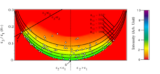
(a)

$\text{WYJ Dalitz Plot}\ \mathcal{E}_{t}=7.5\ \mathrm{eV},\mathcal{P}_{\mathrm{high}}=\sqrt{\frac{14}{47}}$

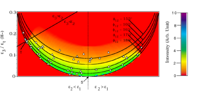
(b)

Figure 8: These original data, obtained directly from the authors, show that as the total center-of-mass energy of the three-body system, ${\mathcal{E}}_{t}$, is increased, a proportionately smaller number of particles undergoes kinematic rearrangement. Shown also are the predicted probability ratios for this rearrangement for the (a) ${\mathcal{E}}_{t}=6.5\ \mathrm{eV}$ and (b) ${\mathcal{E}}_{t}=7.5\ \mathrm{eV}$, triple-coincidence events.

The data (see Figure 8) show a slight asymmetry with small increases in energy (from $6.5\ \mathrm{eV}$ to $7.5\ \mathrm{eV}$) which can be accounted for in a direct manner by considering the local distortion effects herein derived. To see this note that during the nearly co-linear breakup of the excited $H_{3}^{+}$ ion the “initial” proton $H_{i}^{+}$ is emitted in the forward direction and the doubly excited $H^{**}_{2}$ ion is emitted in the backward direction. The subsequent breakup of this ion occurs such that a “final” proton $H^{+}_{f}$ and the nearly equally weighted $H^{-}$ ion are formed.[2] At this point the $H^{-}$ is preferentially associated with $H^{+}_{f}$. However, after the breakup, the continuum pair ($H^{+}_{f},H^{-}$) will acquire a local momentum, $\vec{P}(\vec{r})$, which has a component in the $\hat{r}$ direction. Hence this gained momentum will act to increase the radial separation and will push the $H^{-}$ over the Coulomb Saddle, so that it $H^{-}$ will be preferentially associated with the “initial” proton, $H^{+}_{i}$. Now, because the two protons are in fact indistinguishable, one will observe an asymmetry between “low” and “high” energy scattering events. To help visualize this process, a schematic diagram (see Fig. 9.) has been developed.

Further analysis shows that, as mentioned above, because the local distortion depends upon $\frac{1}{\sqrt{E}}$, as the energy is increased, a proportionately smaller number of particles will experience an impulse that is large enough to alter their final state distribution. Indeed, during the breakup of the $H_{3}^{+}$ ion, the magnitude of the local distortion effects experienced by the ($H^{+}_{f},H^{-}$) continuum pair while in the reaction zone are many orders of magnitude larger than the effects experienced by an electron-proton continuum pair. (see Fig. 10) With this understanding, one may conclude in a straightforward manner, that the observed asymmetry can be attributed to local distortion effects of the three-body system. Moreover, the degree of asymmetry may be predicted as follows:

$$\sqrt{\frac{E_{\mathrm{high}}}{E_{\mathrm{low}}}}\propto\mathrm{\frac{amplitude\ of\ rearrangment\ at\ low\ energy}{amplitude\ of\ rearrangement\ at\ high\ energy}}.$$ (41)

Therefore, with the probabilistic interpretation of the wavefunction, one may write,

$$\sqrt{\frac{E_{\mathrm{high}}}{E_{\mathrm{low}}}}\equiv\sqrt{\mathcal{\frac{P_{\mathrm{low}}}{P_{\mathrm{high}}}}}$$ (42)

where $\mathcal{P}_{\mathrm{high}}$ and $\mathcal{P}_{\mathrm{low}}$ are the probabilities of rearrangement for the high and low energy states, respectively. That is, using the actual data (See Fig. 8.) the ratio of the number of rearranged particles to the total number of detected particles may be calculated. Doing this one obtains the following results:

$$\sqrt{\frac{E_{\mathrm{high}}}{E_{\mathrm{low}}}}=\sqrt{\frac{7.5\ \mathrm{eV}}{6.5\ \mathrm{eV}}}=1.1$$

and

$${\mathcal{\frac{P_{\mathrm{low}}}{P_{\mathrm{high}}}}}=\frac{\sqrt{\frac{31}{72}}}{\sqrt{\frac{14}{47}}}=1.2$$

The absolute error between these two calculations is $\approx 8.7\%$ and illustrates that the generalized local momentum, herein developed may in fact be the actual momentum of the ($H^{-},H^{+}_{f}$) continuum pair during breakup. Indeed, one may consider revaluating the importance of the generalized local momenta. Instead of treating it as a mere mathematical nicety, one may place it on firm physical ground by viewing it is a formal gauge condition for three-body interactions.

6 Towards a Three-Body Gauge

If one grants that the mathematical and computational evidence gathered here, is sufficient to guide further experimental and theoretical investigations by considering the generalized local momentum as a formal three-body gauge condition, then one can construct a three-body gauge transformation. i.e., one may write:

$$\vec{p}\longrightarrow\ \vec{P}(\vec{r})=\vec{p}-\vec{D}_{\vec{P}}(\vec{r}),$$ (43)

when working with three-body systems, in much the same way that one would write,

$$\vec{p}\longrightarrow\ \vec{P}(\vec{r})=\vec{p}-e\hbar\vec{A}(\vec{r}),$$ (44)

when working with particles in an external magnetic field. (i.e., the Coulomb Gauge.)

The subtlety here is that while the transformation,

$$\vec{A}(\vec{r})\longrightarrow\vec{A}(\vec{r})+\vec{\nabla}_{\vec{r}}\Omega(\vec{r})$$

preserves the form of the magnetic field, $\vec{B}(\vec{r})=\vec{\nabla}_{\vec{r}}\times\vec{A}(\vec{r})$, and provides for the global gauge symmetry of the electromagnetic interaction, the condition (43) will contribute a real-valued, position-dependent phase to the relevant wavefunction. Thus any proposed three-body interaction mechanism would require a local gauge symmetry.

To see how a position-dependent phase arises, one may consider a situation similar to that discussed in Sec. 5. That is, consider three-body system consisting of a continuum pair described by the wavefunction, $\Psi_{\vec{p}}(\vec{r})=e^{-i\hbar\vec{p}\cdot\vec{r}}C_{\eta_{p}}(\zeta_{p})$ together with a third, mutually interacting particle. Then, upon breakup, the pair will acquire a local momentum and according to (43), the wavefunction will transform as follows:

$$\Psi_{\vec{p}}(\vec{r})\longrightarrow\Psi_{\vec{P}(\vec{r})}(\vec{r})=e^{-i[\vec{P}(\vec{r})\cdot\vec{r}]}C_{\eta_{p}}(\zeta_{p})=e^{-i\vec{p}\cdot\vec{r}}e^{+i\vec{D}_{\vec{p}}(\vec{r})\cdot\vec{r}}C_{\eta_{p}}(\zeta_{p}).$$ (45)

Using (32d), one then finds that, (for $r\not=0$)

$$\vec{D}_{\vec{p}}(\vec{r})\cdot\vec{r}=a_{0}\eta_{p}\left[1-\cos(\zeta_{p}+2\delta_{\eta_{p}}){}\right]+ia_{0}\eta_{p}\sin(\zeta_{p}+2\delta_{\eta_{p}}).$$ (46)

Therefore the transformed continuum two-body wavefunction takes the following form:

$$\Psi_{\vec{P}(\vec{r})}(\vec{r})=e^{i\vec{p}\cdot\vec{r}}e^{ia_{0}\eta_{p}\left[1-\cos(\zeta_{p}+2\delta_{\eta_{p}})\right]}e^{-a_{0}\eta_{p}\sin(\zeta_{p}+2\delta_{\eta_{p}})}C_{\eta_{p}}(\zeta_{p}),$$ (47)

which shows the explicit form for the position dependent phase. i.e., one may write,

$$S_{\eta_{p}}(\zeta_{p})\equiv ia_{0}\eta_{p}\left[1-\cos(\zeta_{p}+2\delta_{\eta_{p}})\right]-a_{0}\eta_{p}\sin(\zeta_{p}+2\delta_{\eta_{p}}),$$ (48)

and see that the transformation is indeed indicative of a global gauge symmetry. eg.,

$$\Psi_{\vec{P}(\vec{r})}(\vec{r})=e^{S_{\eta_{p}}(\zeta_{p})}\Psi_{\vec{p}}(\vec{r})$$ (49)

It is of course the absolute square of the wavefunction that is truly important for predicting whether or not this phase will significantly effect the experimental findings. To this end, one may take the absolute square of (47) and show that the imaginary-part of the local distortion contributes a real-valued, position-dependent phase. i.e.,

$$\left|\Psi_{\vec{p}}(\vec{r})\right|^{2}=e^{-2a_{0}\eta_{p}\sin(\zeta_{p}+2\delta_{\eta_{p}})}\left|C_{\eta_{p}}(\zeta_{p})\right|^{2}=e^{2\Re S_{\eta_{p}}(\zeta_{p})}\left|C_{\eta_{p}}(\zeta_{p})\right|^{2}.$$ (50)

The exceedingly small magnitude of the term $2a_{0}\eta_{p}\sin(\zeta_{p}+2\delta_{\eta_{p}})$ for the relative energy and reduced masses of the systems considered in current research findings, makes it clear that one may write

$$e^{-2a_{0}\eta_{p}\sin(\zeta_{p}+2\delta_{\eta_{p}})}\longrightarrow 1.$$ (51)

While this reinforces the fact that the proposed framework will leave the asymptotic description of the three-body scattering event unaltered, (as was established in Appendix B) it does not address the extent to which the proposed gauge transformation, (43) will alter the description in the reaction zone.

To begin an investigation of the expected behavior in the reaction zone, one may construct a semi-classical expectation value for the total energy of the continuum pair, $C_{\eta_{p}}(\zeta_{p})$. To do this recall that the expectation value of the semi-classical Hamiltonian for this system (before breakup) would be,

$$\left<H_{0}(\vec{p},\vec{r})\right>=\frac{\hbar^{2}p^{2}}{2\mu}+\frac{Ze^{2}}{4\pi\epsilon_{0}}\frac{1}{r}.$$ (52)

where $p=\frac{\sqrt{2\mu{\mathcal{E}}}}{\hbar}$ is the momentum of the continuum pair before breakup. During breakup, the pair will acquire a local momentum, so that the expectation value of the semi-classical Hamiltonian for the system would then become,

$$\left<H(\vec{P}(\vec{r}),\vec{r})\right>=\frac{\hbar^{2}\left(k^{2}+|\vec{D}_{\vec{p}}(\vec{r})|^{2}\right)}{2\mu}+\frac{Ze^{2}}{4\pi\epsilon_{0}}\frac{1}{r}.$$ (53)

The effects of the proposed gauge transformation may then be observed by plotting the expectation values and varying the relative energy, ${\mathcal{E}}$ (see Fig. 11), the scattering angle, $\theta$ (see Fig. 12), and the reduced mass, $\mu$ (see Fig. 13). All of these show undeniably that while the asymptotic form remains unchanged with respect to variations of all kinematic parameters, genuine three-body distortion effects may arise in the reaction zone. Note specifically that the variation of the relative energy with the scattering reinforces the interpretation offered in Sec. 5. Specifically, the magnitude of the distortion effects for large scattering angles (corresponding to the nearly colinear breakup of the continuum pair) in the reaction zone may cause two opposite-sign-charged particles to increase their radial separation, and appear to repel one another. Conversely, two like-sign-charged particles would decrease their radial separation, and appear to attract one another.

As a last exercise, one may ask if the position-dependent phase introduced by the three-body gauge formalism could be measured. To answer this question one may observe that

$$e^{-2\eta_{p}a_{0}\sin\left(\zeta_{p}+2\delta_{p}\right)}\cong e^{-2\eta_{p}a_{0}}=e^{-\frac{\sqrt{2}za_{0}e^{2}}{4\pi\epsilon_{0}\hbar}\sqrt{\frac{\mu}{e{\mathcal{E}}}}},$$ (54)

where (33) has been used for $\eta_{p}$, and ${\mathcal{E}}$ is measured in electron-volts. As mentioned above, this contribution approaches unity for all systems of physical interest in the realm of current experiments in atomic physics. One can however venture outside of this realm and ask what energy and/or reduced mass is needed to obtain a measurable deviation from unity. If one uses the heaviest purely atomic species, either a proton-proton ($p-p$) or a proton–anti-proton ($p-\bar{p}$) continuum pair, and assumes that a deviation of one part in a million can be measured, then the energy scale needed is on the order of $1\ \mu\mathrm{eV}$! The variation of the term $e^{-2a_{0}\eta_{p}}$ at these energies is shown in Figure 14, and illustrates that one may detect a change in the absolute square of the wavefucntion, thus altering the relevant scattering amplitude. Moreover, the exceedingly small energy scale required to detect these asymptotic distortion effects in either electron(or positron) scattering from hydrogen or in electron-electron or electron-positron ionization processes provides a precise understanding for the success achieved in these areas while ignoring local momentum effects.

7 Conclusion

In the above it has been shown that a generalized, position-dependent local momenta, which depends upon the congugate coordinate through the logarithmic gradient of a continuum state Coulomb wave, may provide evidence for the manifestation of genuine three-body distortion effects in the reaction zone. The form of this local momenta was derived from a consideration of the exact three-body wavefunction, for the case when two of the three, mutually interacting, particles are far apart, and it indicates that the effects do not depend explicitly upon the location of the third particle. For this reason, the effects may be viewed as a distortion of the initial two-body continuum state wavefunction of the two remaining particles. This interpretation was adopted, and it was shown that the local distortion effects could be used to provided a rigorous, physical description of the observed asymmetry in the data obtained by Wiese et. al., [2] on the breakup of three massive Coulomb particles. The degree of this asymmetry was then predicted with an error of less than $10\%$, and it was also shown that while the distortion effects were large in the reaction zone, the asymptotic form of the relevant two-body interaction may be retained by treating the local momentum acquisition as a three-body gauge constraint. Furthermore, the evidence for detecting asymptotic variations in the $\mu\mathrm{eV}$ range, as presented in Fig. 14 suggest that more experimentation be focused on these low energy, heavy-ion–atom processes. Indeed, these experiments may yield new insight into a mechanism by which electrical forces may contribute to the fusion process! That is, the quantum-mechanical–impulse interpretation offered here shows that two like-charged particles may in fact attract one another due to local distortion effects in the reaction zone.

In addition to these findings and predictions, one may learn much by noting that by adopting the proposed three-body gauge transformation, one finds that an electron-proton continuum pair exhibited a very small amount of distortion in the reaction zone. This result provides a rigorous explanation of why the paradigm 3C wavefunction works so well for light-ion–atom scattering [6],[9]. Moreover, the general framework shows that an electron-electron continuum pair would experience distortion effects of lesser magnitude, due to its greatly decreased reduced mass. These results can again be used to explain why Qiu et. al.,[10] achieved amazing success in modeling electron-electron photo-ionization processes, while ignoring local momentum effects. Indeed, if one recalls the path-integral interpretation suggested in Sec. 5, then the success of these findings for light-ion–atom processes may be attributed to the fact that the leading contribution to the relevant cross sections are the “paths” along which the local distortion effects are identically zero. While no analytic form exists for calculation of these roots, one can compile a table for use in numerical calculations and construct a solution that better reflects the physical nature of the three-body interaction.

Appendix A The Logarithmic Derivative of the ${}_{1}F_{1}(i\eta_{p},1;-1\zeta_{p})$ Function

The logarithmic derivative of the confluent hypergeometric function is defined here as follows:

$$\vec{D}_{\vec{p}}(\vec{r}) \equiv i\vec{\nabla}_{r}\ln{{}_{1}F_{1}\left(i\eta_{p},1;-i\zeta_{p}\right)}=i\frac{\vec{\nabla}_{r}{}_{1}F_{1}(i\eta_{p},1;-i\zeta_{p})}{{}_{1}F_{1}(i\eta_{p},1;-i\zeta_{p})}$$

$$= i\eta_{p}{}p\frac{{}_{1}F_{1}\left[(i\eta_{p}+1),2;-i\zeta_{p}\right]}{{}_{1}F_{1}(i\eta_{p},1;-i\zeta_{p})}(\hat{p}+\hat{r}).$$

Then using the well known recursion relationship,(See reference [7] for instance.)

$$\frac{z}{b}{}_{1}F_{1}\left[(a+1),(b+1),z\right]={}_{1}F_{1}\left[(a+1),b,z\right]-{}_{1}F_{1}\left(a,b,z\right),$$ (56)

one may write

$$\vec{D}_{\vec{p}}(\vec{r}) = i\eta_{p}{p}\frac{\left[{}_{1}F_{1}\left[(i\eta_{p}+1),1;-i\zeta_{p}\right]-{}_{1}F_{1}(i\eta_{p},1;-i\zeta_{p})\right]}{\zeta_{p}{}_{1}F_{1}(i\eta_{p},1;-i\zeta_{p})}(\hat{p}+\hat{r}),\quad\quad\quad\zeta_{p}>0.$$ (57)

Further simplification of the logarithmic derivative is obtained by use of the Kummer relation[7] for the confluent hypergeometric equation. e.g.,

$${}_{1}F_{1}\left(a,b,z\right)=e^{z}{}_{1}F_{1}\left[(b-a),b,-z\right].$$ (58)

With this relation one finds that the distortion may be rewritten as follows:

$$\vec{D}_{\vec{p}}(\vec{r}) = i\eta_{p}{p}\frac{\left[e^{-i\zeta_{p}}{}_{1}F_{1}(-i\eta_{p},1;i\zeta_{p})-{}_{1}F_{1}(i\eta_{p},1;-i\zeta_{p})\right]}{\zeta_{p}\ {}_{1}F_{1}(i\eta_{p},1;-i\zeta_{p})}(\hat{p}+\hat{r})$$ (59a)

$$= \frac{\eta_{p}}{r\ \hat{p}\cdot(\hat{p}+\hat{r})}\left[1-e^{-i\zeta_{p}}\frac{{}_{1}F_{1}(-i\eta_{p},1;i\zeta_{p})}{{}_{1}F_{1}(i\eta_{p},1;-i\zeta_{p})}\right](\hat{p}+\hat{r}),\quad\quad\quad{}r>0.$$ (59b)

At this point note that the ratio of confluent hypergeometric equations in equation (59b) is in fact a very special case because the function on top is the complex conjugate of the function on the bottom! i.e.,

$${}_{1}F_{1}(-i\eta_{p},1;i\zeta_{p})={{}_{1}F_{1}}^{{\dagger}}(i\eta_{p},1;-i\zeta_{p}),$$ (60)

so that one may define a real-valued, position-dependent phase,

$$\tan\left[\delta_{\eta_{p}}(\zeta_{p})\right]=\frac{\Im\left[{}_{1}F_{1}(i\eta_{p},1;-i\zeta_{p})\right]}{\Re\left[{}_{1}F_{1}(i\eta_{p},1;-i\zeta_{p})\right]}.$$ (61)

The logarithmic derivative may then be written as follows:

$$\vec{D}_{\vec{p}}(\vec{r})=\Bigg{\{}\begin{tabular}[]{c}$i\eta_{p}{p}(\hat{p}+\hat{r}),\quad r=0$\\ $\frac{\eta_{p}}{r}\left[1-e^{-i(\zeta_{p}+2\delta_{\eta_{p}}(\zeta_{p}))}\right]\frac{(\hat{p}+\hat{r})}{\hat{p}\cdot(\hat{p}+\hat{r})},\quad r>0$\end{tabular},$$ (62)

and one sees that in this form, the local distortion is analytic everywhere, except possibly at $r=0$. This result is very significant, because it allows one to investigate the nature of the local momenta well inside of the interior regions of a scattering event in a rigorous manner. Only in this way can one determine the relative importance of these local effects.

Appendix B An Alternative Three-Body Wavefunction

To solve equation (3) for the unknown function $\chi_{\vec{k}_{\alpha},\vec{q}_{\alpha}}(\vec{r}_{\alpha},\vec{\rho}_{\alpha})$ one normally assumes that the interaction energy (cf, equation (26)) satisfies

$${\mathcal{E}_{I}}=0.$$

This technique was developed by Popalilios as referenced in [6], and asserts that the total center of mass energy of the three-body system is partitioned among the two reduced mass clusters, $\mu_{\alpha}$ and $M_{\alpha}$. Hence one may write

$$\left[-\frac{\hbar^{2}}{2\mu_{\alpha}}\vec{\nabla}^{2}_{\vec{r}_{\alpha}}-i\frac{\hbar}{\mu_{\alpha}}\vec{K}(\vec{r}_{\alpha})\cdot\vec{\nabla}_{\vec{r}_{\alpha}}-\frac{\hbar^{2}}{2M_{\alpha}}\vec{\nabla}^{2}_{\vec{\rho}_{\alpha}}-i\frac{\hbar}{M_{\alpha}}\vec{Q}(\vec{\rho}_{\alpha})\cdot\vec{\nabla}_{\vec{\rho}_{\alpha}}+V_{\alpha}^{I}(\vec{r}_{\alpha},\vec{\rho}_{\alpha})\right]\chi_{\vec{k}_{\alpha},\vec{q}_{\alpha}}(\vec{r}_{\alpha},\vec{\rho}_{\alpha})=0.$$ (63)

and see that $\chi_{\vec{k}_{\alpha},\vec{q}_{\alpha}}(\vec{r}_{\alpha},\vec{\rho}_{\alpha})$ must be built to incorporate each term in the interaction potential.

To accomplish this, assume that $\chi_{\vec{k}_{\alpha},\vec{q}_{\alpha}}(\vec{r}_{\alpha},\vec{\rho}_{\alpha})$ is given by

$$\chi_{\vec{k}_{\alpha},\vec{q}_{\alpha}}(\vec{r}_{\alpha},\vec{\rho}_{\alpha})=C_{-\eta_{q_{\alpha}}}(\zeta_{q_{\alpha}})f_{\beta}(\vec{r}_{\alpha},\vec{\rho}_{\alpha})f_{\gamma}(\vec{r}_{\alpha},\vec{\rho}_{\alpha}),$$ (64)

where $C_{-\eta_{q_{\alpha}}}(\zeta_{q_{\alpha}})$ satisfies

$$\left[-\frac{\hbar^{2}}{2M_{\alpha}}\vec{\nabla}^{2}_{\vec{\rho}_{\alpha}}-i\frac{\hbar}{M_{\alpha}}\vec{q}_{\alpha}\cdot\vec{\nabla}_{\vec{\rho}_{\alpha}}-\frac{Z_{\alpha}(Z_{\beta}+Z_{\gamma})e^{2}}{4\pi\epsilon_{0}}\frac{1}{\rho_{\alpha}}\right]C_{\eta_{q_{\alpha}}}(\zeta_{q_{\alpha}})=0.$$ (65)

Because the function $C_{-\eta_{q_{\alpha}}}(\zeta_{q_{\alpha}})$ is a known function, which exactly incorporates the interaction term $-\frac{Z_{\alpha}(Z_{\beta}+Z_{\gamma})e^{2}}{4\pi\epsilon_{0}\rho_{\alpha}}$, this substitution results in the following (exact) coupled equations for the functions $f_{\nu}(\vec{r}_{\nu},\vec{\rho}_{\nu})$:($\nu=\beta,\gamma$)

$$\leavevmode\resizebox{361.34999pt}{}{$\left[-\frac{\hbar^{2}}{2\mu_{\alpha}}\vec{\nabla}^{2}_{\vec{r}_{\alpha}}-\frac{\hbar^{2}}{2M_{\alpha}}\vec{\nabla}^{2}_{\vec{\rho}_{\alpha}}-i\frac{\hbar}{\mu_{\alpha}}\vec{K}_{\alpha}^{\gamma}(\vec{r}_{\alpha};\vec{r}_{\gamma},\vec{\rho}_{\gamma})\cdot\vec{\nabla}_{\vec{r}_{\alpha}}-i\frac{\hbar}{M_{\alpha}}\vec{Q}_{\alpha}^{\gamma}(\vec{\rho}_{\alpha},\vec{r}_{\gamma},\vec{\rho}_{\gamma})\cdot\vec{\nabla}_{\vec{\rho}_{\alpha}}+V_{\nu,\mathrm{eff}}^{(\gamma)}(\vec{r}_{\beta},\vec{\rho}_{\alpha})\right]f_{\beta}(\vec{r}_{\beta},\vec{\rho}_{\beta})=0$},$$ (66a)

$$\leavevmode\resizebox{361.34999pt}{}{$\left[-\frac{\hbar^{2}}{2\mu_{\alpha}}\vec{\nabla}^{2}_{\vec{r}_{\alpha}}-\frac{\hbar^{2}}{2M_{\alpha}}\vec{\nabla}^{2}_{\vec{\rho}_{\alpha}}-i\frac{\hbar}{\mu_{\alpha}}\vec{K}_{\alpha}^{\beta}(\vec{r}_{\alpha};\vec{r}_{\beta},\vec{\rho}_{\beta})\cdot\vec{\nabla}_{\vec{r}_{\alpha}}-i\frac{\hbar}{M_{\alpha}}\vec{Q}_{\alpha}^{\beta}(\vec{\rho}_{\alpha},\vec{r}_{\beta},\vec{\rho}_{\beta})\cdot\vec{\nabla}_{\vec{\rho}_{\alpha}}+V_{\gamma,\mathrm{eff}}^{(\beta)}(\vec{r}_{\gamma},\vec{\rho}_{\alpha})\right]f_{\gamma}(\vec{r}_{\gamma},\vec{\rho}_{\gamma})=0$},$$ (66b)

where (for $\epsilon\not=\nu$, with $\epsilon=\beta,\gamma$)

$$\vec{K}_{\alpha}^{\epsilon}(\vec{r}_{\alpha};\vec{r}_{\epsilon},\vec{\rho}_{\epsilon}) = \vec{k}_{\alpha}-i\vec{\nabla}_{\vec{r}_{\alpha}}\ln C_{\eta_{k_{\alpha}}}(\zeta_{k_{\alpha}})-\frac{i}{2}\vec{\nabla}_{\vec{r}_{\alpha}}\ln f_{\epsilon}(\vec{r}_{\epsilon},\vec{\rho}_{\epsilon}),$$ (67a)

$$\vec{Q}_{\alpha}^{\epsilon}(\vec{\rho}_{\alpha};\vec{r}_{\epsilon},\vec{\rho}_{\epsilon}) = \vec{q}_{\alpha}-i\vec{\nabla}_{\vec{\rho}_{\alpha}}\left[\ln C_{\eta_{q_{\alpha}}}(\zeta_{q_{\alpha}})C_{-\eta_{q_{\alpha}}}(\zeta_{q_{\alpha}})\right]-\frac{i}{2}\vec{\nabla}_{\vec{\rho}_{\alpha}}\ln f_{\epsilon}(\vec{r}_{\epsilon},\vec{\rho}_{\epsilon}),$$ (67b)

and

$$V_{\nu,\mathrm{eff}}^{(\epsilon)}(\vec{r}_{\nu},\vec{\rho}_{\alpha})=\frac{Z_{\alpha}Z_{\epsilon}e^{2}}{4\pi\epsilon_{0}}\frac{1}{r_{\nu}}\times\left\{1+\frac{4\pi\epsilon_{0}\eta_{q_{\alpha}}^{2}}{Z_{\alpha}Z_{\epsilon}e^{2}M_{\alpha}}\left(\frac{r_{\nu}}{\rho_{\alpha}}\right)\left[1-e^{-i(\zeta_{q_{\alpha}}+2\delta_{\eta_{q_{\alpha}}}(\zeta_{q_{\alpha}}))}\right]\left[1-e^{-i(\zeta_{q_{\alpha}}+2\delta_{-\eta_{q_{\alpha}}}(\zeta_{q_{\alpha}}))}\right]\right\}.$$ (68)

While these equations may seem even more complicated than the original equation, there are many important aspects to note:

• The effective potential reduces to the Coulomb potential for the $\nu$-channel, in the asymptotic regions $\Omega_{0}$ and $\Omega_{\alpha}$. i.e.,

  $$V_{\nu,\mathrm{eff}}^{(\epsilon)(\Omega_{0},\Omega_{\alpha})}(\vec{r}_{\nu},\vec{\rho}_{\alpha})=\frac{Z_{\alpha}Z_{\epsilon}e^{2}}{4\pi\epsilon_{0}}\frac{1}{r_{\nu}}$$ (69)

• The second term in $\vec{Q}_{\alpha}^{\epsilon}(\vec{\rho}_{\alpha},\vec{r}_{\epsilon},\vec{\rho}_{\epsilon})$ vanishes in the asymptotic regions because,

  $$\left[C_{\eta_{q_{\alpha}}}(\zeta_{q_{\alpha}})C_{-\eta_{q_{\alpha}}}(\zeta_{q_{\alpha}})\right]_{\lim_{{\rho_{\alpha}}\to\infty}}\longrightarrow e^{-i\eta_{q_{\alpha}}\ln\zeta_{q_{\alpha}}}e^{+i\eta_{q_{\alpha}}\ln\zeta_{q_{\alpha}}}=1.$$ (70)

  (Indeed, this cancellation of the logarithmic phases was “built in” to the solution!)

• The first two terms in $\vec{K}_{\alpha}^{\epsilon}(\vec{r}_{\alpha},\vec{r}_{\epsilon},\vec{\rho}_{\epsilon})$ may be identified as a position-dependent, local momentum. i.e.,

  $$\vec{K}_{\alpha}(\vec{r}_{\alpha})=\vec{k}_{\alpha}-i\vec{\nabla}_{\vec{r}_{\alpha}}\ln C_{\eta_{k_{\alpha}}}(\zeta_{k_{\alpha}}).$$

• The solutions are coupled in a completely symmetric way by the terms $-\frac{i}{2}\vec{\nabla}_{\vec{r}_{\alpha}}\ln f_{\nu}(\vec{r}_{\epsilon},\vec{\rho}_{\epsilon})$ and
  $-\frac{i}{2}\vec{\nabla}_{\vec{\rho}_{\alpha}}\ln f_{\nu}(\vec{r}_{\epsilon},\vec{\rho}_{\epsilon})$, so that a numerical solution of these equations would be manifestly less computationally intensive.

Furthermore, because the equations (66) are exact, they would be more reliable in ab initio calculations.

Approximate solutions that are valid through second order, may be achieved in a direct manner following the techniques outlined in [12] and may be written in the form of distorted and coupled Coulomb waves. e.g.,

$$f_{\nu}(\vec{r}_{\nu},\vec{\rho}_{\nu})=C_{\eta_{K_{\nu}^{\epsilon}}}(\zeta_{K_{\nu}^{\epsilon}})\equiv\Gamma(1-i\eta_{K_{\nu}^{\epsilon}})e^{-\frac{\pi\eta_{K_{\nu}^{\epsilon}}}{2}}{}_{1}F_{1}\left(i\eta_{K_{\nu}^{\epsilon}},1,-i\zeta_{K_{\nu}^{\epsilon}}\right),$$ (71)

where the conventional, two-body normalization procedure has been employed so that that incoming wave has unit magnitude.

The complete three-body wavefunction may then be written in the form:

$$\Psi_{\vec{k}_{\alpha},\vec{q}_{\alpha}}^{KC5C}(\vec{r}_{\alpha},\vec{\rho}_{\alpha})=e^{i(\vec{k}_{\alpha}\cdot\vec{r}_{\alpha}+\vec{q}_{\alpha}\cdot\vec{\rho}_{\alpha})}C_{\eta_{k_{\alpha}}}(\zeta_{k_{\alpha}})C_{\eta_{q_{\alpha}}}(\zeta_{q_{\alpha}})C_{-\eta_{q_{\alpha}}}(\zeta_{q_{\alpha}})C_{\eta_{K_{\beta}^{\gamma}}}(\zeta_{K_{\beta}^{\gamma}})C_{\eta_{K_{\gamma}^{\beta}}}(\zeta_{K_{\gamma}^{\beta}})$$ (72)

a product of five, kinematically coupled Coulomb waves. To see that this solution is valid, first note that one can show in a straightforward manner that the distorted Coulomb waves have the following asymptotic form:

$$C_{\eta_{K_{\nu}^{\epsilon}}}^{(\Omega_{0})}(\zeta_{K_{\nu}^{\epsilon}})\rightarrow C_{\eta_{k_{\nu}}}(\zeta_{k_{\nu}})$$ (73)

Hence, due to the relationship (70), the asymptotic form in $\Omega_{0}$ will be identical to that of the Redmond, 3C wavefunction.

The Jacobi Coordinates

\psfrag{ra}{\Large$\vec{r}_{\alpha}$}\psfrag{rb}{\Large$\vec{r}_{\beta}$}\psfrag{rc}{\Large$\vec{r}_{\gamma}$}\psfrag{pa}{\Large$\vec{\rho}_{\alpha}$}\psfrag{pb}{\Large$\vec{\rho}_{\beta}$}\psfrag{pc}{\Large$\vec{\rho}_{\gamma}$}\psfrag{ma}{\Large$m_{\alpha}$}\psfrag{mb}{\Large$m_{\beta}$}\psfrag{mc}{\Large$m_{\gamma}$}\includegraphics{jacobi.eps}

Figure 1: The Jacobi coordinates are most often used to study many-body kinematics, because any orthogonal pair, $(\vec{r}_{\nu},\vec{\rho}_{\nu}),\quad\nu=\alpha,\beta,\gamma$ may be used. See equations (1) for the definition of the reduced masses.

         ${\mathcal{E}}$ Dependence of the Local Distortion

\psfrag{r}[bc]{$r\ (a_{0})$}\psfrag{D}[bc]{$\Re D_{\vec{p}}(\vec{r})\ (\frac{1}{p})$}\psfrag{Re}{$\Re$}\psfrag{Im}{$\Im$}\psfrag{eV}{$\mathrm{eV}$}\includegraphics{vare.eps}

Figure 2: The real part of the local distortion experienced by an electron-proton continuum pair with relative energies as indicated and a scattering angle of $\theta=4^{\circ}$.

         $\mu$ and $Z$ Dependence of the Local Distortion

\psfrag{r}[bc]{$r\ (a_{0})$}\psfrag{D}[bc]{$\Re D_{\vec{p}}(\vec{r})\ (\frac{1}{p})$}\psfrag{ee}{$e-\bar{e}$}\psfrag{ep}{$e-p$}\includegraphics{varm.eps}

Figure 3: The real part of the local distortion experienced by both electron-electron and electron-proton continuum pairs, with values as in Fig. 2. Note that the sign of the distortion is different for the attractive $(e^{-},p^{+})$ and repulsive $(e^{-},e^{-})$ cases.

         Stationary Points of the Local Distortion

\psfrag{r}[bc]{$r\ (a_{0})$}\psfrag{D}[bc]{$D_{\vec{p}}(\vec{r})\ (\frac{1}{p})$}\psfrag{Re}{$\Re$}\psfrag{Im}{$\Im$}\includegraphics{station.eps}

Figure 4: The local distortion experienced by an electron-proton continuum pair with a relative energy of $10\ \mathrm{eV}$, and a scattering angle of $\theta=16^{\circ}$. Note that when the zeroes of real and imaginary part of the distortion coincide, the distortion contribution will be identically zero.

Topology of the Local Distortion

\psfrag{C}[bc]{\rotatebox{90.0}{$\Re D_{\vec{p}}(\vec{r})\ (\frac{1}{p})$}}\psfrag{r}{$r\ (a_{0})$}\psfrag{theta}{$\theta$}\psfrag{Dep}{$\Re D$}\includegraphics{visual1.eps}

(a)

\psfrag{C}[bc]{\rotatebox{90.0}{$\Re D_{\vec{p}}(\vec{r})\ (\frac{1}{p})$}}\psfrag{r}{$r\ (a_{0})$}\psfrag{theta}{$\theta$}\psfrag{Dep}{$\Re D$}\includegraphics{visual2.eps}

(b)

Figure 5: Shown here are (a) three-dimensional and (b) contour plots of the real part of the local distortion experienced by an electron-proton continuum pair with a relative energy of $10\ \mathrm{eV}$.

         Local Distortion Phase Effects

\psfrag{r}[bc]{$r\ (a_{0})$}\psfrag{delta}[bc]{$\delta_{\eta_{p}}(\zeta_{p})$}\psfrag{theta}{$\theta=20^{\circ}$}\psfrag{eV}{$\mathrm{eV}$}\includegraphics{delta.eps}

Figure 6: Shown here is the position dependent-phase, $\delta_{\eta_{p}}(\zeta_{p})$. Note that it is very nearly constant over one log-cycle and that it is nearly independent of the relative energy of the electron-proton continuum pair.

Local Distortion Effects for Various Continuum Pairs

$$\begin{array}[]{cc}{\leavevmode\resizebox{144.54pt}{}{\includegraphics[bb=0 350 285 540]{e-e+.eps}}}&{\leavevmode\resizebox{144.54pt}{}{\includegraphics[bb=0 350 285 540]{e-e-.eps}}}\\ {\leavevmode\resizebox{144.54pt}{}{\includegraphics[bb=0 350 285 540]{e-p+.eps}}}&{\leavevmode\resizebox{144.54pt}{}{\includegraphics[bb=0 350 285 540]{e+p+.eps}}}\\ {\leavevmode\resizebox{144.54pt}{}{\includegraphics[bb=0 350 285 540]{p-p+.eps}}}&{\leavevmode\resizebox{144.54pt}{}{\includegraphics[bb=0 350 285 540]{p+p+.eps}}}\end{array}$$

Figure 7: Shown are the local distortion effects experienced by (a) electron-positron, (b) electron-electron, (c) electron-antiproton , (d) positron-proton, (e) proton-antiproton, and (f) proton-proton, continuum pairs with ${\mathcal{E}}=10\ \mathrm{eV}$ and $\theta=16^{\circ}$. While these effects become negligible asymptotically, the effects become more pronounced in the interior regions; the range has been shortened in (e) and (f) to show the dramatic change due to the increase in the reduced mass of the pair

$\text{WYJ Dalitz Plot}\ \mathcal{E}_{t}=6.5\ \mathrm{eV},\mathcal{P}_{\mathrm{low}}=\sqrt{\frac{31}{72}}$

Explanation of Three-Body Distortion Effects

\psfrag{H3}{$(H_{3}^{+})^{*}$}\psfrag{H2}{$H_{2}^{**}$}\psfrag{Hip}{$H_{i}^{+}$}\psfrag{Hfp}{$H_{f}^{+}$}\psfrag{Hm}{$H^{-}$}\psfrag{Hp}{$H^{+}$}\psfrag{p}{$\vec{p}$}\psfrag{r}{$\vec{r}$}\psfrag{Pr}{$\vec{P}(\vec{r})$}\psfrag{CS}[bc]{Coulomb\ Saddle}\psfrag{Low}[bc]{Low\ Energy}\psfrag{High}[bc]{High\ Energy}\psfrag{a}{(a)}\psfrag{b}{(b)}\psfrag{c}{(c)}\psfrag{d}{(d)}\includegraphics[bb=5 5 600 785]{explain.eps}

Figure 9: (a) During the breakup of the $H_{3}^{+}$ ion the $H_{i}^{+}$ is emitted in the forward direction and the $H^{**}_{2}$ is emitted in the backward direction. (b) The subsequent breakup of this ion occurs such that the $H^{+}_{f}$ and $H^{-}$ ions are formed, and the $H^{-}$ is preferentially associated with $H^{+}_{f}$. (c) The continuum pair, ($H^{+}_{f},H^{-}$) acquires a local momentum, $\vec{P}(\vec{r})$, pushing the $H^{-}$ over the Coulomb Saddle, so that the $H^{-}$ will be associated with the $H^{+}_{i}$. (d) Because the two protons are in fact indistinguishable, one will observe an asymmetry between “low” and “high” energy scattering events.

      $\text{Distortion Effects During}\ (H_{3}^{-})^{*}\ \text{Breakup}$

\psfrag{title}[bc]{}\psfrag{eV}{}\psfrag{r}[bc]{$r\ (a_{0})$}\psfrag{dist}[bc]{$\Re D_{\vec{p}}(\vec{r})\ (\frac{1}{p})$}\includegraphics[bb=0 350 290 535]{breakup.eps}

Figure 10: During the breakup of the $H_{3}^{+}$ ion, the magnitude of the local distortion effects experienced by the ($H^{+}_{f},H^{-}$) continuum pair while in the reaction zone are many orders of magnitude larger than the effects experienced by either the ($e,\bar{e}$) or ($e,e$) continuum pairs. Here $\theta=176^{\circ}$ and ${\mathcal{E}}=1.5\ \mathrm{eV}$ for comparison with the experiment.

Three-Body Gauge Variation with ${\mathcal{E}}$

\psfrag{r}{$r\ (a_{0})$}\psfrag{E}{$\mathcal{E}$}\psfrag{title}{}\psfrag{mass}{}\psfrag{theta}{}\psfrag{eV}[bc]{Relative Energy}\psfrag{H}{$H$}\psfrag{H0}{$H_{0}$}\includegraphics[bb=0 350 285 540]{evar1.eps}

(a)

\psfrag{r}{$r\ (a_{0})$}\psfrag{E}{$\mathcal{E}$}\psfrag{title}{}\psfrag{mass}{}\psfrag{theta}{}\psfrag{eV}[bc]{Relative Energy}\psfrag{H}{$H_{0}$}\psfrag{H0}{$H$}\includegraphics[bb=0 350 285 540]{evar2.eps}

(b)

\psfrag{r}{$r\ (a_{0})$}\psfrag{E}{$\mathcal{E}$}\psfrag{title}{}\psfrag{mass}{}\psfrag{theta}{}\psfrag{eV}[bc]{Relative Energy}\psfrag{H}{$H_{0}$}\psfrag{H0}{$H$}\includegraphics[bb=0 350 285 540]{evar3.eps}

(c)

Figure 11: The effects of the three-body gauge transformation are shown to depend critically upon the relative energy of the continuum pair. Observe that as the relative energy of an electron-proton continuum pair, with a scattering angle of $\theta=0^{\circ}$, is increased from (a) ${\mathcal{E}}=3\ \mathrm{eV}$ to (b) ${\mathcal{E}}=10\ \mathrm{eV}$ to (c) ${\mathcal{E}}=54.4\ \mathrm{eV}$, the effects in the reaction zone nearly vanish.

Three-Body Gauge Variation with $\theta$

\psfrag{r}{$r\ (a_{0})$}\psfrag{H}{$H_{0}$}\psfrag{H0}{$H$}\psfrag{E}{$\mathcal{E}$}\psfrag{title}{}\psfrag{mass}{}\psfrag{theta}{}\psfrag{eV}[bc]{Relative Energy}\psfrag{H}{$H_{0}$}\psfrag{H0}{$H$}\includegraphics[bb=0 350 285 540]{avar1.eps}

(a)

\psfrag{r}{$r\ (a_{0})$}\psfrag{H}{$H_{0}$}\psfrag{H0}{$H$}\psfrag{E}{$\mathcal{E}$}\psfrag{title}{}\psfrag{mass}{}\psfrag{theta}{}\psfrag{eV}[bc]{Relative Energy}\psfrag{H0}{$H_{0}$}\psfrag{H}{$H$}\includegraphics[bb=0 350 285 540]{avar2}

(b)

\psfrag{r}{$r\ (a_{0})$}\psfrag{H}{$H_{0}$}\psfrag{H0}{$H$}\psfrag{E}{$\mathcal{E}$}\psfrag{title}{}\psfrag{mass}{}\psfrag{theta}{}\psfrag{eV}[bc]{Relative Energy}\psfrag{H0}{$H_{0}$}\psfrag{H}{$H$}\includegraphics[bb=0 350 285 540]{avar3.eps}

(c)

Figure 12: The effects of the three-body gauge transformation are shown to depend critically upon the scattering angle of the continuum pair. Observe that as the scattering angle of an electron-proton continuum pair, with a relative energy of ${\mathcal{E}}=10\ \mathrm{eV}$, is increased from (a) $\theta=0^{\circ}$ to (b) $\theta=75^{\circ}$ to (c) $\theta=150^{\circ}$, the effects in the reaction zone become more pronounced.

Three-Body Gauge Variation with $\mu$

\psfrag{r}{$r\ (a_{0})$}\psfrag{E}{$\mathcal{E}$}\psfrag{title}{}\psfrag{mass}{}\psfrag{theta}{}\psfrag{eV}[bc]{Relative Energy}\psfrag{H}{$H_{0}$}\psfrag{H0}{$H$}\includegraphics[bb=0 350 285 540]{mvar1.eps}

(a)

\psfrag{r}{$r\ (a_{0})$}\psfrag{E}{$\mathcal{E}$}\psfrag{title}{}\psfrag{mass}{}\psfrag{theta}{}\psfrag{eV}[bc]{Relative Energy}\psfrag{H}{$H$}\psfrag{H0}{$H_{0}$}\includegraphics[bb=0 350 285 540]{mvar2}

(b)

\psfrag{r}{$r\ (a_{0})$}\psfrag{E}{$\mathcal{E}$}\psfrag{title}{}\psfrag{mass}{}\psfrag{theta}{}\psfrag{eV}[bc]{Relative Energy}\psfrag{H}{$H_{0}$}\psfrag{H0}{$H$}\includegraphics[bb=0 350 285 540]{mvar3.eps}

(c)

Figure 13: The effects of the three-body gauge transformation are shown to depend critically upon the reduced mass of the continuum pair. Observe that as the reduced mass of the continuum pair, with a relative energy of ${\mathcal{E}}=10\ \mathrm{eV}$ and a scattering angle of $\theta=0^{\circ}$, is increased from (a) $\mu=1\mu_{ep}$ to (b) $\mu=10\mu_{ep}$ to (c) $\mu=20\mu_{ep}$, the effects in the reaction are dramatically altered.

Asymptotic Phase Variation

\psfrag{title}{}\psfrag{phase}{$e^{-2a_{0}\eta_{p}}$}\psfrag{E}{${\mathcal{E}}\ (\mathrm{\mu eV})$}\psfrag{pp}{$p-p$}\psfrag{pap}{$p-\bar{p}$}\includegraphics[bb=0 300 330 490]{ppvar.eps}

(a)

\psfrag{title}{}\psfrag{phase}{$e^{-2a_{0}\eta_{p}}$}\psfrag{E}{${\mathcal{E}}\ (\mathrm{neV})$}\psfrag{ep}{$e-p$}\psfrag{aep}{$\bar{e}-p$}\includegraphics[bb=0 300 330 490]{epvar.eps}

(b)

\psfrag{title}{}\psfrag{phase}{$e^{-2a_{0}\eta_{p}}$}\psfrag{E}{${\mathcal{E}}\ (\mathrm{peV})$}\psfrag{ee}{$e-e$}\psfrag{aee}{$e-\bar{e}$}\includegraphics[bb=0 300 330 490]{eevar.eps}

(c)

Figure 14: Shown is the variation of the phase achieved by the three-body gauge transformation (see text equation (43)) for (a) a proton-proton or proton–anti-proton, (b) an electron-proton or positron-proton and (c) electron-electron or electron-positron continuum pair. Observe that as the reduced mass of the system is decreased accordingly, the corresponding energy decrease is sufficient to detect a variation of one part in a million.

References

• [1] E. O. Alt and A. M. Mukhamedzhanov, Phys. Rev. A $\mathbf{47}$, 2004(1993).
• [2] L. Wiese et. al., PRL $\mathbf{79}$, 4982 (1997).
• [3] P.P Fiziev, T. Y. Fizieva, Few-Body Systems $\mathbf{2}$ 71 (1987).
• [4] P. J. Redmond, ca. 1972,unpublished (as referenced by Rosenberg).
• [5] L. Rosenberg, Phys. Rev. D $\mathbf{8}$, 1833(1972). $\mathbf{56}$, 370(1997).
• [6] M. Brauner et. al., J. Phys. B $\mathbf{22}$, 2265(1989).
• [7] I. S. Gradshteyn and I. M. Ryzhik, Table of Integrals, Series, and Products. Academic Press, London (1965).
• [8] J. Berakdar, J. S. Briggs, Phys. Rev. A
• [9] S. Jones and D. Madison, Phys. Rev. A $\mathbf{55}$ 444 (1997).
• [10] Y. Qiu et. al., Phys. Rev. A $\mathbf{57}$, R1489 (1998).
• [11] M. Lieber and A. M. Mukhamedzhanov, Phys. Rev. A $\mathbf{54}$, 3078(1996).
• [12] A. Engelns et. al,, J. Phys. B $\mathbf{(}30)$, L811(1997).