SOLITON GENERATION AND PICOSECOND COLLAPSE IN SOLID-STATE LASERS WITH SEMICONDUCTOR SATURABLE ABSORBER

International Laser Center, 65 Skorina Ave., Bldg. 17, Minsk, 220027 BELARUS, e-mail: vkal@ilc.unibel.by, http://www.geocities.com/optomaplev

Abstract. Based on self - consistent field theory we study a soliton generation in cw solid-state lasers with semiconductor saturable absorber. Various soliton destabilizations, i.e. the switch from femtosecond to picosecond generation (”picosecond collapse”), an automodulation regime, breakdown of soliton generation and hysteresis behavior, are predicted. It is shown that the third-order dispersion reduces the region of the soliton existence and causes the pulse oscillation and strong frequency shift.

OCIS codes: 140.7090, 140.3430, 190.5530

1 Introduction

Recent advances in ultrafast solid-state lasers have resulted in sub 6-fs pulses generated directly from the cavity of Ti: sapphire laser [1], which is close to the theoretical limit for optical pulses. The key role to mode-locking in this case plays the fast optical nonlinearities, such as electronic nonlinearities, responsible, in particular, for self-phase modulation (SPM) and self-focusing [2].

As was shown, the generation of extremely short pulses in the lasers with self-focusing or semiconductor saturable absorber [3] is possible due to formation of a Schrödinger soliton. The relevant mechanism is the balance between SPM and group velocity dispersion (GVD), which reduces the pulse duration and stabilizes it. This mechanism termed the soliton mode-locking [4] works together with Kerr-lensing or saturable absorption of semiconductor thus supporting the ultrashort pulse and preventing from the noise generation. However, the presence of dissipative laser factors, such as saturable gain and loss, frequency filtering etc., complicates the soliton dynamics essentially, so that various nonstationary regimes in Kerr-lens mode-locked lasers [5, 6] and Q-switching instability in the cw lasers with semiconductor saturable absorber [7] are possible. Up to now a theoretical understanding of the above-mentioned issues is lacking and challenges for investigators efforts, that can be of particular interest for the for generation dynamics and pulse characteristics control in femtosecond region.

Here we present the results of our study of the soliton generation in cw solid-state lasers with semiconductor saturable absorber. The main focus of investigation was set on the peculiarities of the transition between femtosecond (soliton) and picosecond generation. We shall demonstrate that such a transition is accompanied by the threshold and hysteresis phenomena. Based on soliton perturbation theory, the numerical simulations of two different experimental situations have been performed. The first one corresponds to the variation of control parameters (dispersion or pump power), when for every new value of control parameter the laser is turned on afresh. The second situation is for continuous variation of control parameter during a single generation session. We demonstrate also that the third order dispersion destabilizes the soliton and produces a strong frequency shift of generation wavelength with respect to the gain center.

2 Model

We analyzed the field evolution in the distributed laser system containing saturable quasi-four level gain crystal, frequency filter, GVD and SPM elements, two level saturable absorber and linear loss. We assumed, that in noncoherent approximation the saturable absorber action can be described by operator $-\frac{\gamma\exp(-E/E_{s})}{1+\partial/\partial t}$ [8], where $\gamma$ is the initial saturable loss, $E=\int\limits_{-\infty}^{t}\left|a(t\prime)\right|^{2}dt\prime\;$is the energy fluency passed through the absorber to moment $t$, $t$ is the local time, $E_{s}$ is the loss saturation energy fluency; the expansion of the denominator into the time series in $\frac{\partial}{\partial t}$ is further supposed. The gain saturation is due to the full pulse energy. The ratio of the loss saturation energy to the gain saturation energies $\tau$ under assumption of the equal cross sections of the generation mode at semiconductor modulator and Ti: sapphire active medium is $1.25\times 10^{-4}$ for $E_{s}=100\;\mu J/cm^{2}$ (compare this with the figure for semiconductor saturation energy reported in [3]).

The evolution of generation field a obeys the following operator equation:

$$\frac{\partial a(z,t)}{\partial z}=\left[\alpha\exp(-\tau E)-\frac{\gamma\exp(-E)}{1+\frac{\partial}{\partial t}}+\left[\frac{1}{1+\frac{\partial}{\partial t}}-1\right]-l\right]a(z,t)$$

$$+\left[ik_{2}\frac{\partial^{2}}{\partial t^{2}}+k_{3}\frac{\partial^{3}}{\partial t^{3}}-i\beta\left|a(z,t)\right|^{2}\right]a(z,t)$$ (1)

were $z$ is the longitude coordinate normalized to the cavity length, or transit number, $\alpha$ is the saturated gain, $l$ is the linear loss, $k_{2,3}$ are the second- and third-order dispersion coefficients, respectively, the energy fluency is normalized to $E_{s}$ . The time is normalized to the inverse bandwidth of the absorber $1/t_{a}$ . With this normalization the SPM coefficient $\beta$ is $\frac{2\pi n_{2}LE_{s}}{\lambda nt_{a}}$, where $L$ is the length of crystal, $n$ and $n_{2}$ are the linear and nonlinear coefficients of refractivity, respectively, $\lambda$ is the generation wavelength. The term in square parenthesis stands for the frequency filtering. The transmission band of the filter and the absorption band of semiconductor were assumed to coincide. An expansion of Eq. (1) up to second-order in $\partial/\partial t$ results in nonlinear Landau-Ginzburg equation [4, 8], which we do not write out here due to its complexity.

Since an exact general solution of Eq. (1) is unknown, we sought for the approximated quasi-soliton solution in the form $a(z,t)=a_{0}\frac{\exp\left[i\omega(t-z\delta)+i\varphi z\right]}{\cosh\left[(t-z\delta)/t_{p}\right]^{1+i\Psi}}$, where $a_{0}$ is the amplitude, $t_{p}$ is the width, $\omega$ is the frequency mismatch from filter band center, $\Psi$ is the chirp, $\varphi$ and $\delta$ are the phase and time delays after the full cavity round trip, respectively. In the frame of aberrationless approach [9], the substitution of this solution in Eq. (1) with following expansion in $t$ yields the following set of ordinary differential equations for evolution of pulse parameters:

$$\frac{da_{0}}{dz} = a_{0}\left[\begin{array}[]{c}\alpha\exp\left(-\frac{\tau a_{0}^{2}}{v}\right)+\left(1-\omega^{2}-v^{2}\right)\gamma\exp\left(-\frac{a_{0}^{2}}{v}\right)-l+k_{2}\Psi v^{2}-\\ \omega^{2}-v^{2}-3k_{3}\omega v^{2}\Psi\end{array}\right],$$ (4)

$$\frac{d\omega}{dz} = \left(\Psi a_{0}^{2}\omega^{2}+a_{0}^{2}\omega-2v^{2}\omega-2v^{2}\omega\Psi^{2}-\Psi a_{0}^{2}\right)\gamma\exp\left(-\frac{a_{0}^{2}}{v}\right)-$$

$$2v^{2}\omega\Psi^{2}-2v^{2}\omega-\Psi a_{0}^{2}\tau\alpha\exp\left(-\frac{\tau a_{0}^{2}}{v}\right)-3k_{3}v^{4}\Psi\left(\Psi^{2}+1\right),$$

$$\frac{dv}{dz} = \frac{1}{2v^{2}}\left(a_{0}^{4}v^{2}+2v^{4}\Psi^{2}-a_{0}^{4}+a_{0}^{4}\omega^{2}+2a_{0}^{2}v^{2}-4a_{0}^{2}\omega v^{2}\Psi-4v^{4}\right)\times$$

$$\gamma\exp\left(-\frac{a_{0}^{2}}{v}\right)-\frac{a_{0}^{4}\tau^{2}\alpha}{2v^{2}}\exp\left(-\frac{\tau a_{0}^{2}}{v}\right)+3k_{2}v^{2}\Psi+v^{2}\Psi^{2}-$$

$$2v^{2}-9k_{3}\omega\Psi v^{2},$$

$$\frac{d\Psi}{dz} = \left(4a_{0}^{2}\omega v^{2}+a_{0}^{4}\Psi+4a_{0}^{2}\omega v^{2}\Psi^{2}-2v^{4}\Psi-\Psi a_{0}^{4}\omega^{2}-a_{0}^{4}\omega-2v^{4}\Psi^{3}\right)\times$$

$$\frac{\gamma}{v^{2}}\exp\left(-\frac{a_{0}^{2}}{v}\right)+\frac{\Psi\alpha a_{0}^{4}\tau^{2}}{v^{2}}\exp\left(-\frac{\tau a_{0}^{2}}{v}\right)-2a_{0}^{2}\beta-2v^{2}\Psi-$$

$$4k_{2}v^{2}\Psi^{2}-2v^{2}\Psi^{3}-4k_{2}v^{2}+12k_{3}\omega v^{2}\left(\Psi^{2}+1\right),$$

where $v=1/t_{p}$ is the inverse pulse width, and the solutions for time and phase delays:

$\delta=\left[a_{0}^{2}\left(\omega^{2}+v^{2}-1)-2v^{2}\omega\Psi\right)\right]\gamma\exp\left(-\frac{a_{0}^{2}}{v}\right)-2\omega\Psi v^{2}-2k_{2}\omega v^{2}+$

$k_{3}v^{2}\left(5v^{2}+3\omega^{2}-3v^{2}\Psi^{2}\right)-a_{0}^{2}\tau\alpha\exp\left(-\frac{\tau a_{0}^{2}}{v}\right),$

$\varphi=\left[a_{0}^{2}\omega\left(\omega^{2}+v^{2}-1\right)+v^{2}\Psi\left(v^{2}-2\omega^{2}\right)\right]\gamma\exp\left(-\frac{a_{0}^{2}}{v}\right)+k_{3}v^{2}\omega\times$

$\left(2v^{2}+2\omega^{2}-3v^{2}\Psi^{2}\right)+k_{2}v^{2}\left(v^{2}-\omega^{2}\right)+\Psi v^{4}+\beta a_{0}^{2}v^{2}-2\omega^{2}\Psi v^{2}-$

$\omega\tau\alpha a_{0}^{2}\exp\left(-\frac{\tau a_{0}^{2}}{v}\right).$

Assuming that pulse width is much shorter than the cavity period $T_{cav}$ , the equation for the gain evolution is as follows:

$$\frac{d\alpha}{dz}=\left(\alpha_{m}-\alpha\right)P-\frac{2\alpha\tau a_{0}^{2}}{v}-\frac{\alpha}{T_{g}},$$ (6)

where $P=\frac{\sigma T_{cav}I_{p}}{h\upsilon}$ is the dimensionless pump intensity, $\sigma$ is the absorption cross-section at the pump wavelength, $h\upsilon$ is the energy of pump photon, $\alpha_{m}$ is the maximal gain at the full population inversion. $P=10^{-4}$ corresponds to the pump power of 1W for $100\;\mu m$ diameter of pump mode.

The steady-state solution of Eqs. (2, 3) describes the stable ultrashort pulses generation. The system (2, 3) was solved by the forward Euler method with number of iterations $\leavevmode\nobreak\ 10^{6}$ and the accuracy of $\leavevmode\nobreak\ 10^{-6}$ .

3 Discussion

First, we shall study the situation when for each new value of control parameter the generation is formed starting from the noise spike as initial approximation.

The normalized width of the stable pulse versus GVD coefficient is presented in Fig. 1 for different amount of SPM. It is well known that in solid-state lasers contrary to the dye lasers a soliton mode locking with a slow saturable absorber is impossible because of small contribution of dynamic gain saturation (a small $\tau$ in our notations) but at the same time the presence of SPM can provide the stable soliton mode locking [4]. As was expected, our calculations confirmed this conclusion for the situation with no SPM present in the system. However, with some SPM another pulse stabilizing mechanism comes to play a role. Introducing the SPM stabilizes the picosecond generation (region A in Fig. 1) due to the action of negative feed-back [8] (top-left segment of curve 1 in Fig. 2). The mechanism of this feed-back is as follows: an increased pulse intensity causes a stronger chirping, i.e. a wider pulse spectrum and, consequently, a higher loss at bandwidth limiting element and, reverse, a decreased intensity minimizes the chirp and the spectral width, reducing the loss at spectral filter.

There is a section at the curves 1-4 (Fig. 1, 2) where the Schrödinger soliton exists within limited window of negative dispersion. The pulse durations lie in femtosecond region with the minimum close to zero GVD, the pulse intensities are much higher and the chirp is very small (central part of curve 1 in Fig. 2). Calculation showed that contrary to ps-case and the situation with non-zero third-order dispersion the soliton has no frequency shift from filter band center and its energy is equal to critical energy for first-order Schrödinger soliton $E=\frac{2\left|k_{2}\right|}{t_{p}\beta}$ .

At some negative GVD the switch from femtosecond to picosecond regime (”picosecond collapse” marked by arrow, see curve 1 in Fig. 1) takes place. Formally, these two types of ultrashort generation correspond to domination of either nondissipative (case of Schrödinger soliton generation) or dissipative (case of picosecond generation) terms in Eq. 1, respectively.

For the stronger SPM (curve 2 in Fig. 1) the interval of GVD, where the femtosecond generation takes place, broadens which is accompanied by the shortening of the pulse width (compare curves 1 and 2 in Figs. 1, 2). As is seen, the ps-collapse occurs now at much higher (both in negative and positive region) dispersions.

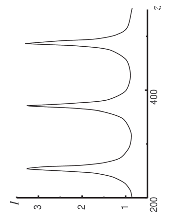
Figure 3: Peak intensity $I$ normalized to $E_{s}t_{a}^{-1}$ versus round-trip number $z$. $k_{2}=-20$ , $k_{3}=0$ , $P=5\times 10^{-4}$ , $\beta$ $=0.05$.

Further increasing of SPM transforms the character of soliton destabilization (curve 3 in Fig. 1). In this case, the femtosecond generation is possible only near zero dispersion; the higher negative GVD destroys the soliton-like pulse (discontinuity of curve 3). Left to the region where no quasi-soliton solution for Eq. 1 exists, there appears the region of the pulse automodulational instability (region B). Here, the pulse parameters oscillate with the period of $\sim$ $100$ cavity round-trips ($\sim 1$ $\mu s$ ) as is illustrated in Fig. 3. The oscillating pulse has quasi-Schrödinger soliton type with a small chirp (region B in Fig. 2) and frequency shift.

Further increase of SPM (curve 4 in Fig. 1) reduces the interval of quasi-soliton existence. Comparing curves 1 - 4 of Fig. 1 one may conclude that the optimal amount of SPM exists providing the femtosecond generation in the widest interval of GVD.

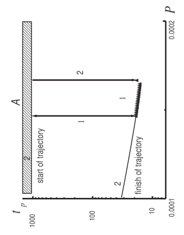
Figure 4: Pulse width $t_{p}$ versus pump intensity $P$. Arrow 1 - switch between ps- and fs-generation (triangles). $k_{2}=-10$ , $k_{3}=0$ , $\beta$ $=0.1$, other parameters correspond to Fig. 1.

Let’s consider the pump intensity $P\;$- another control parameter of the system switching the generation between ps- and fs-regimes. As is seen from Fig. 4 (triangles and arrow 1), the increase of the pump switches the laser from ps- to fs-generation. This occurs when the pump intensity and, consequently, the generation pulse intensity becomes high enough for SPM to compensate the GVD.

We can investigate the system behavior depending on control parameters (pump, GVD) by two different cases. First one is when we measure the pulse characteristics at the some value of control parameters then turn off the laser where upon turn on the laser and iterate this process with another value of control parameter. Mathematically it corresponds to receiving of the pulse as stationary solution of Eq. 1 from the noise spike. This case is depicted at Figs. 1, 2 and triangles in Fig. 4. Second case is when one receives ultrashort pulse at the definite value of the control parameter and then begins smooth variation of this parameter. This case is depicted at Fig. 4, b and Fig. 5.

As is seen from Fig. 4, the dependence of the pulse duration on the pump intensity demonstrates a hysteresis behavior. The pump variation from the small values to the large and backward produces the following sequence of generation regimes (trajectory 2 in Fig. 4): the pump increase from $10^{-4}$ to $2\times 10^{-4}$ does not bring the system from ps- to fs-generation, however the subsequent pump decrease from $2\times 10^{-4}$ to $1.67\times 10^{-4}$ switches the system to fs-regime. The range of fs-generation in terms of $P$ (solid curve) is wider than for the case denoted by triangles, which was plotted analogous to curves of Figs. 1 and 2. If the trajectory starts from large $P$, the picosecond regime does not set and the femtosecond soliton forms at $P\approx 1.67\times 10^{-4}$ (solid curve). In this case, the interval of the soliton existence is wider than for regime denoted by triangles.

The system demonstrates the hysteresis behavior under the variation of GVD, too (Fig. 5): changing the GVD from the negative values to zero and than to the positive values does not cause the switch from ps- to fs-generation. On the other hand when moving from the positive values of dispersion to negative and backwards one can see the dramatic change in system’s behavior. The decrease of GVD starting from the positive values, where the ps-generation takes place, causes an abrupt switch to fs-generation near zero GVD. Comparing curve 2 in Fig. 1 and the curve in Fig. 5 that were plotted for the same parameters but for different physical situations (described above), one may conclude that the region of the soliton existence is wider in term of GVD for the latter case (when we alter the GVD) than for the former (when generation is formed from the noise spike). The switch from fs to ps generation under inverse movement along the GVD axis takes place at another value of GVD thus producing a hysteresis feature (see Fig. 5).

Since the Schrödinger soliton formation occurs at small negative GVD, the contribution of third-order dispersion $k_{3}$ in this region may be essential. The presence of $k_{3}\neq 0$ gives rise to the following effects: 1) the strong pulse frequency shift which depends on the sign of $k_{3}$ (compare curves 2, 3 and 4 and curve 1 in Fig. 6) arises; 2) the region of fs-generation narrows; 3) an additional destabilizing factor, the frequency shift oscillations, appears (regions B for curves 2, 3, 4).

4 Conclusion

In summary, based on the self-consistent field theory we have investigated the characteristics of Schrödinger soliton in cw solid-state laser with semiconductor saturable absorber. We demonstrated numerically, that the formation of soliton has threshold character, so together with first (free running) and second (mode-locking) threshold the threshold of femtosecond generation exists. Three main destabilization scenarios were demonstrated: the switch to picosecond generation (picosecond collapse), the switch to automodulation mode and the breakdown of soliton-like pulse. The switch between pico- and femtosecond generation has the hysteresis character. The contribution of high-order GVD reduces the interval of quasi-soliton existence, gives rise to the frequency shift and the pulse destabilization.

Our results may be useful for design of self-starting cw solid-state lasers with controllable ultrashort pulse characteristics.

This work was supported by National Foundation for basic researches (grant F97-256).

5 References

1. D. H. Sutter, G. Steinmeyer, L. Gallmann, N. Matuschek, F. Morier-Genoud, and U. Keller, ”Semiconductor saturable-absorber mirror’s assisted Kerr-lens mode-locked Ti:sapphire laser producing pulses in the two-cycle regime”, Opt. Lett., 24, 631-633 (1999).

2. H. Haus, J. G. Fujimoto, and E. P. Ippen, ”Analytic theory of additive pulse and Kerr lens mode locking”, IEEE J. Quant. Electr., 28, 2086-2095 (1995).

3. U. Keller, K. J. Weingarten, F. X. Kärtner, D. Kopf, B. Braun, I. D. Jung, R. Fluck, C. Hönninger, N. Matuschek, and J. A. der Au, ”Semiconductor saturable absorbers mirrors (SESAM’s) for femtosecond to nanosecond pulse generation in solid-state lasers”, IEEE J. Selected Topics in Quant. Electr., 2, 435-451 (1996).

4. F. X. Kärtner, I. D. Jung, and U. Keller, ”Soliton mode-locking with saturable absorbers”, IEEE J. Selected Topics in Quant. Electr., 2, 540-555 (1996).

5. S. R. Bolton, R. A. Jenks, C. N. Elkinton, G. Sucha, ”Pulse-resolved measurements of subharmonic oscillations in a Kerr-lens mode-locked Ti: sapphire laser”, J. Opt. Soc. Am. B, 16, 339-344 (1999).

6. V. L. Kalashnikov, I. G. Poloyko, V. P. Mikhailov, D. von der Linde, ”Regular, quasi-periodic and chaotic behavior in cw solid-state Kerr-lens mode-locked lasers”, J. Opt. Soc. Am. B, 14, 2691-2695 (1997).

7. C. Hönninger, R. Paschotta, F. Morier-Genoud, M. Moser, and U. Keller, ”Q-switching stability limits of continuous-wave passive mode locking”, J. Opt. Soc. Am. B, 16, 46-56 (1999).

8. V. L. Kalashnikov, D. O. Krimer, I. G. Poloyko, V.P. Mikhailov, ”Ultrashort pulse generation in cw solid-state laser with semiconductor saturable absorber in the presence of the absorption linewidth enhancement”, Optics Commun., 159, 237-242 (1999).

9. A. M. Sergeev, E. V. Vanin, F. W. Wise, ”Stability of passively modelocked lasers with fast saturable absorbers”, Optics Commun., 140, 61-64 (1997).

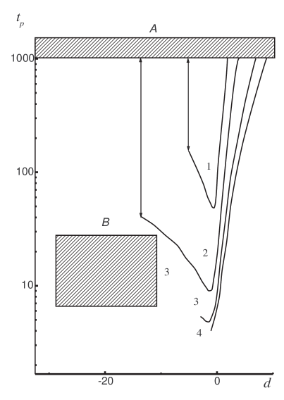
Figure 1: Pulse width $t_{p}$ versus GVD coefficient $k_{2}$ (time is normalized to $t_{a}$ ). Region A, picosecond generation, region B, autooscillation regime for parameters of curve 3. $P=5\times 10^{-4}$ , $\alpha_{m}=0.5$ , $t_{a}=2.5\;fs$, $T_{g}$ $=3$ $\mu s$ , $T_{cav}=10\;ns$, $l=0.01$, $\gamma=0.05$ , $k_{3}=0$ . $\beta$ $=0.001$ (1), $0.01$ (2), $0.05$ (3), $0.1$ (4).

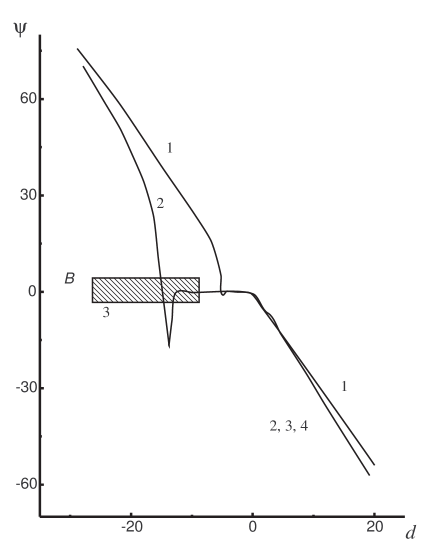
Figure 2: Chirp $\Psi$ versus GVD coefficient $k_{2}$ . The parameters correspond to Fig. 1. Curve 3 and 4 exist under $k_{2}\geq\;-3$,$\;-1$, respectively.

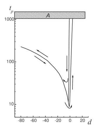
Figure 5: Pulse width $t_{p}$ versus GVD coefficient $k_{2}$ . Parameters correspond to curve 2 in Fig.1.

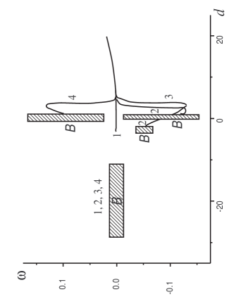
Figure 6: Frequency shift $\omega$ versus GVD coefficient $k_{2}$ . Parameters correspond to curve 3 in Fig. 1. $k_{3}=0$ (1), $-5$ (2), $-10$ (3), $10$ (4). The initial conditions correspond to Figs. 1, 2.