Noise Delays Bifurcation in a Positively Coupled Neural Circuit

Abstract

We report a noise induced delay of bifurcation in a simple pulse-coupled neural circuit. We study the behavior of two neural oscillators, each individually governed by saddle-node dynamics, with reciprocal excitatory synaptic connections. In the deterministic circuit, the synaptic current amplitude acts as a control parameter to move the circuit from a mono-stable regime through a bifurcation into a bistable regime. In this regime stable sustained anti-phase oscillations in both neurons coexist with a stable rest state. We introduce a small amount of random current into both neurons to model possible randomly arriving synaptic inputs. We find that such random noise delays the onset of bistability, even though in decoupled neurons noise tends to advance bifurcations and the circuit has only excitatory coupling. We show that the delay is dependent on the level of noise and suggest that a curious stochastic “anti-resonance” is present.
PACS numbers: 87.10.+e,87.18.Bb,87.18.Sn,87.19.La

I Introduction

The effects of random currents on the firing behavior of real and model neurons have received a considerable amount of attention in neurobiology and physics literature [1, 2, 3, 4, 5, 6, 7, 8]. Several experimental results indicate that in vivo neural spike trains seem to be excessively noisy, with interspike interval distribution showing 1/f spectra [9]. However, other in vitro experiments have shown that noisy stimuli can produce highly reliable firing with the neuron locking onto large range variations of the noise [2, 10]. A number of theoretical studies have attempted to reconcile such seemingly disparate results by studying the dynamics of neural networks with additive noise, showing that high variance firing behavior can arise in networks of threshold elements [12]. At the same time additive noise in oscillating networks of more realistic neurons destabilizes synchronous and phase locked behavior, producing complicated spatiotemporal patterns [13]. These simulation results have appeared in the context of a body of literature that has delved into the effects of noise on the response of excitable and oscillatory non-linear dynamical systems. In particular a number of investigators have considered what happens to single neurons and circuits of neurons when noise perturbs periodically modulated input signals. Experimental work has identified noise induced signal amplification and resonance in a number of preparations e.g. [14]. Theoretical analyses have successfully explained such findings employing the language of stochastic resonance developed originally for general multi-stable dynamical systems. There the enhancement of the subthreshold stimuli and encoding of stimulus structure had a non-linear relationship with the noise amplitude, resulting in a signal-to-noise ratio relationship with a pronounced peak. Noise effects have also been studied in the context of indigenous oscillations in neural models, focusing on the so-called “autonomous stochastic resonance” [5]. For example, a recent report by Lee shows noise induced coherence resonance in a Hodgkin-Huxley model, with pre-cursors of the sub-critical Hopf bifurcation revealed by the action of random currents [6]. In this sense noise “advanced” the bifurcation. Similar effects have also been found in a generic saddle-node driven oscillator where noise advances the onset of oscillations and upregulates the mean frequency [15, 16]

Although pulse coupled or synaptically coupled neural networks have received much recent attention with regard to their dynamics [17, 18] and computational power [19], we believe that this Letter is the first attempt to look in detail at the effects of noise on the onset of synaptically sustained firing in such networks. That is, circuits of intrinsically quiescent neurons where activity occurs purely due to the recurrent synaptic interactions. To our knowledge, almost all efforts to study the interplay of noise and neural oscillators report noise induced increase in firing and advancement of bifurcations, e.g. [15]. In this light our finding is rather intriguing since we observe a noise induced delay of bifurcation in a purely positively coupled circuit of neural oscillators. We also observe a phenomenon that may be termed “stochastic anti-resonance”, since the delay of bifurcation depends non-linearly on the noise level. Our analysis of this system leads us to conclude that the relative width of the attractor basins for the quiescent and persistent firing states is the key factor in determining whether stochastic resonance has a delaying, neutral, or advancing effect on the bifurcation.

Below we summarize the dynamics of the spiking neuron used in this circuit (the $\theta$-neuron), and analyze the case of two coupled cells in the regimes of weak and strong excitatory coupling in both noise free and noisy simulations. Since we believe that the phenomenon we observe is generic for circuits of recurrently coupled spiking neurons, first we describe the stochastic anti-resonance phenomenon observed in this simple circuit.

Figure 1A, upper trace shows the firing patterns of two cells whose spiking behavior results from mutual excitatory synapses. The cells are initially quiescent (they are not intrinsically spiking) and their activity results from an initial external input to one cell. Activity can be terminated by small levels of noise (Figure 1A, middle trace), whilst increased noise levels cause intermittent firing (Figure 1A, lower trace). Figure 1B plots the probability ($M_{1}$) of observing firing in the last 200 msecs of a 2000 msec run over an ensemble of 1000 sample paths. The x-axis plots the strength of the synaptic coupling ($g_{s}$). In the noise free circuit, $g_{s}^{*}$ is the critical value of coupling above which sustained firing occurs (i.e. $M_{1}$=0 for $g_{s}<g_{s}^{*}$, $M_{1}$=1 for $g_{s}\geq g_{s}^{*}$). Since the synaptically sustained firing apears with a non-zero frequency, we suspect that the bifurcation here is of a sub-critical Hopf type. At small noise levels (Figure 1B, traces 1,2), increasing the noise amplitude progressively shifts the curves of $M_{1}$ to the right with respect to the noise-free case. This behavior is surprising as addition of small amounts of noise for a single autonomously spiking $\theta$-neuron induces the opposite effect - noise advanced bifurcation (see [21]). The effect has been described in a generic saddle-node oscillator in [15]. Above a critical noise value, the onset of sustained firing is advanced back to the left (Figure 1B, traces 3 and higher). Thus the bifurcation is delayed for low noise amplitudes and advanced with higher noise. Figure 1C shows that there is a non-linear relationship between the amount of injected noise and the firing probability. Here we plot the value of $g_{s}=g_{s}^{2/3}$ at which continuous sustained firing is observed in 2/3 of the sample paths, the same points are marked on the probability plots in Figure 1B. Adding small amounts of noise moves the probability curves to the right. This can be viewed as a probabilistic signature of a delay of the bifurcation. As the noise amplitude grows, the bifurcation is delayed further, and the test point $g_{s}^{2/3}$ occurs at higher $g_{s}$ values. As the noise is increased further, noise fluctuations are strong enough to induce intermittent firing. Both the probability curves and the location of the test point then move back to the left towards the noise-free value. If we consider the sustained firing as signal (perturbed by noise), this resembles stochastic resonance, however here the net effect of noise is “negative”.

It should be noted that this effect is not restricted to the dynamics of the $\theta$-neuron. All aspects of noise induced delay of bifurcation seen above also occur in a circuit where each of the cells is modeled with a more complicated conductance based, Hodgkin-Huxley model for a pyramidal neuron [11] (simulations not shown). This is not surprising, since this model can be readily reduced to the $\theta$-neuron which we now describe.

II The $\theta$-neuron

The $\theta$-neuron model developed by Ermentrout and Gutkin [20, 21] is derived from the observation that wide class of neuronal models of cortical neurons, based on the electrophysiological model of Hodgkin and Huxley show a saddle-node type bifurcation at a critical parameter value. This parameter determines the dynamical behavior of the solutions of the corresponding system of ordinary differential equations. General dynamical systems theory tells us that the qualitative behavior in some neighborhood of the bifurcation point (which may be quite large as it extends up to the next bifurcation or other dynamic transition) is governed by the reduction of the system to the center manifold. In the present case of the saddle-node bifurcation which is the simplest bifurcation type, this leads to the following differential equation

$$\frac{dx}{dt}=\lambda+x^{2}.$$ (1)

Here, the bifurcation parameter $\lambda$ is considered as the input to the neuron while $x$ records its activity. Obviously, a solution to this equation tends to infinity in finite time. This is considered as a spiking event, and the initial values are then reset to $-\infty$. In order to have a model that does not exhibit such formal singularities, one introduces a phase variable $\theta$ that is $2\pi$-periodic via

$$x=\tan(\frac{\theta}{2}).$$ (2)

$\theta$ is then a variable with domain the unit circle $S^{1}$, and a spike now corresponds to a period of $\theta$. Spikes are no longer represented by transitions through infinity, but by changes of some discrete topological invariant. The original differential equation is then transformed into

$$\frac{d\theta}{dt}=(1-\cos(\theta))+(1+\cos(\theta))\lambda.$$ (3)

Due to the nonlinearity of the transformation from $x$ to $\theta$, the input $\lambda$ is no longer additive. In fact, it is easy to show that $(1+cos\theta)$ is the phase resetting function for the model [20]. As before, the bifurcation occurs at $\lambda=0$. There, we have precisely one rest point, namely $\theta=0$ which is degenerate. In any case, the sensitivity to the input $\lambda$ is highest at $\theta=0$ and lowest at $\theta=\pi$ which according to the derivation of our equation is considered as the spike point. When $\lambda$ is positive, the equation does not have any rest point. In this case, $\theta$ continues to increase all the time, and the neuron is perpetually firing. When $\lambda$ is negative, however, there are two rest points, a stable one denoted by $\theta_{r}$ and an unstable one $\theta_{t}>\theta_{r}$. If $\theta$ is larger than $\theta_{t}$ it increases until it completes a period and comes to rest at $\theta_{r}+2\pi$ which is identified with $\theta_{r}$ as we are working on the unit circle $S^{1}$. Thus, if the phase is above the threshold value $\theta_{t}$, a spike occurs and the neuron returns to rest. So far, we have tacitly assumed that the input $\lambda$ is constant. We now consider the situation where the input can be decomposed as

$$\lambda=\beta+\sigma\eta,$$ (4)

where $\beta$ is a constant term, the so-called bias, while $\eta$ is (white) noise and $\sigma$ its intensity. In this case, sufficiently strong noise can occasionally push the phase $\theta$ beyond the threshold value $\theta_{t}$ causing intermittent firing (Figure 1C). Equation 3 now becomes a canonical stochastic saddle-node oscillator which has been studied in Rappel & Wooten and Gutkin & Ermentrout [21].

III Coupled neurons

We now consider the situation where we have two neurons (distinguished by subscripts $i=1,2$). The dynamics then takes place on the product of two circles, i.e. on a two-dimensional torus $T$, represented by the square $[-\pi,\pi]\times[-\pi,\pi]$ in the plane, with periodic boundary identifications. We first consider the simple case of two uncoupled, noise-free neurons ($\sigma_{1}=\sigma_{2}=0$) with the same bias $\beta$. Their dynamics are independent. In the phase plot shown in Figure 2(i) the diagonal is always an invariant curve, corresponding to synchronized activity of the two neurons. If $\beta>0$, both neurons continue to fire, although their phase difference, if not 0 initially, is not constant, due to the nonlinearity of the differential equation governing it. If $\beta=0$, $(0,0)$ is a degenerate rest point (Figure 2(ii)). The two curves $\theta_{1}=\theta_{2}=0$ are homoclinic orbits and all flow lines eventually terminate at this fixed point. One or both neurons will spike before returning to rest if their initial phase is between 0 and $\pi$.

If $\beta<0$ (Figure 2(iii)), we have four fixed points - the attractor $(\theta_{1}=\theta_{2}=\theta_{r})$, the repeller $(\theta_{1}=\theta_{2}=\theta_{t})$, and the two saddles where one of the neurons has its phase at $\theta_{r}$ (rest) and the other one at $\theta_{t}$ (threshold). Some special heteroclinic orbits are given by the straight lines where one of the two neurons stays at $\theta_{t}$ while the other one moves from the threshold to the rest value, spiking if its initial phase was above threshold. All other flow lines terminate at the attractor. We now add an interaction term $s_{i}g_{s}$ to the input of neuron $i$. $s_{i}$ is considered as the synaptic input from neuron $j$ to neuron $i$ ($i\neq j$) and $g_{s}$ is the synaptic intensity. (One could also study the case of a single neuron $i$ for which $s_{i}$ represents synaptic self-coupling, but here we are interested in the case of two coupled neurons). A precise equation for $s_{i}$ can be derived from electrophysiological models, however for our qualitative study we only need the characteristic features that it stays bounded between 0 and 1. Typically, it is peaked near the spike of neuron $j$, i.e. where $\theta_{j}=\pi$. With this interaction term, the equation for neuron $i$ then becomes

$$\frac{d\theta_{i}}{dt}=(1-\cos(\theta_{i}))+(1+\cos(\theta_{i}))(\beta+g_{s}s_{i}+\sigma\eta).$$ (5)

Since $s_{i}$ represents the input that neuron $i$ receives from neuron $j$, $s_{i}$ should essentially be considered as a function of the phase $\theta_{j}$ of $j$. Once more, we first consider the situation without noise, i.e. $\sigma=0$ (although our final aim is to understand the effect of noise on the dynamic behavior of the coupled neurons). We also assume that we are in the excitable region, i.e. $\beta<0$. $g_{s}$ is assumed to be positive (excitatory coupling), and so the coupling counteracts the effect of the bias to a certain extent, a crucial difference being, however, that the synaptic input to each neuron is time dependent, in contrast to the constant bias. If $g_{s}$ is sufficiently small, the qualitative situation does not change compared to the case without coupling, i.e. $g_{s}=0$. We still have a heteroclinic orbit from the saddle $(\theta_{1}=\theta_{t},\theta_{2}=\theta_{r})$ to the attractor $(\theta_{r},\theta_{r})$, although $\theta_{2}$ does not stay constant anymore along that orbit, but increases first a little due to the input from neuron 1 before it descends again to the rest value. (Figure 2(iv)). (Of course, we also get such an orbit with the roles of the two neurons reversed; in fact, the dynamical picture is always invariant under reflection across the diagonal, i.e.under exchanging the two neurons.) If $g_{s}$ reaches some critical value $g_{s}^{*}$, however, the heteroclinic orbit starting at $(\theta_{t},\theta_{r})$ does not terminate anymore at the attractor, and the value of the phase of neuron 2 is increased so much by the synaptic interaction that it reaches the other saddle $(\theta_{r},\theta_{t})$ (Figure 2v). Besides two heteroclinic orbits that go from the repeller to the two saddles as before, all other orbits still terminate at the attractor $(\theta_{r},\theta_{r})$, for $g_{s}=g_{s}^{*}$. If $g_{s}$ is increased beyond $g_{s}^{*}$, however, the heteroclinic orbit between the two saddles mutates into a stable attractor (Figure 2(vi)). It corresponds to sustained asynchronous firing of the two neurons. In fact, if the phase difference between the two neurons is too small, the dynamics converges towards the double rest point (except in some region in the vicinity of the node), and both neurons stop firing. This is caused by the fact that when the two neurons are close to synchrony, neither cell is sensitive enough to its synaptic input to maintain firing (an effective refractory period). Conversely, if they are out of synchrony, a single spike can induce the second neuron to fire at a time when the first one is close to rest, and sensitive to synaptic input itself. If $g_{s}$ is only slightly above the critical value, the basin of attraction of that limit cycle will still be relatively small, but as $g_{s}$ is increased further, the basin grows in size until eventually it is larger than the basin of attraction of the double rest point. On the basis of the preceding analysis, it is now straightforward to predict the effect of noise. If $g_{s}$ is only slightly above the critical value $g_{s}^{*}$, a small amount of noise is more likely to kick the dynamics out of the narrow basin of attraction of the asynchronous limit cycle and into the large basin of the double rest point than vice versa. In effect, a small noise level increases the critical parameter value required for the qualitative transition to sustained asynchronous firing. A larger amount of noise, however, has the potential to move the dynamics from the rest point into the basin of attraction of the asynchronous limit cycle. Once in that basin, the neurons will fire. Thus, for large noise in that regime, one will observe that the neurons will fire, perhaps with some intermissions spent near the double rest point. So, a larger value of noise will cause intermittent periods of sustained firing of the two neurons even at somewhat smaller values of $g_{s}$. In effect, it decreases the value of the critical parameter. Thus, we observe a genuinely nonlinear effect of the noise level $\sigma$ (Figure 1E). For values of the coupling $g_{s}$ that are substantially larger than the critical value $g_{s}^{*}$, even small amounts of noise have a good chance of perturbing the dynamics out of the attracting vicinity of the double rest point into the attracting region of the asynchronous limit cycle. This will further enhance the sustained asynchronous firing pattern of the two neurons.

IV Conclusions

In this work we report a new and unusual effect of noise in a simple neural circuit. When the sustained oscillations in the circuit are induced by recurrent excitatory coupling, small noise levels can exert a strong influence on the circuit dynamics, often abolishing the firing. The probability of observing sustained firing has been used to characterize the transition from quiescent to oscillatory behavior. Figure 1B clearly shows that in this system, noise delays this transition. Noise induced delay of bifurcation can therefore occur in a completely positively coupled circuit. The same noise has the exact opposite effect of advancing the bifurcation when it is applied to a single autonomously firing neuron. The paradoxical effect of noise in this circuit can be understood by considering the structure of its phase plane - and in particular the width of the attractor basins for the sustained antiphase oscillations. When the width of the attractor basin is small, small levels of noise can perturb the system into the larger basin of the stable quiescent state. However, transitions in the opposite direction from the rest-state to a sustained firing state can only occur when noise fluctuations reach a critical value. Above this value, transitions into the firing state begin to counteract transitions into the quiescent state. Alternatively, as the coupling strength increases, the basin of attraction for the sustained firing solution grows at the expense of the quiescent state. The negative (bifurcation-delaying) effect of the noise is then eliminated. In this system low levels of noise effectively act as a switch to turn off otherwise continuous firing behavior. Alternatively, low levels of noise ensure that sustained firing can only take place above a critical coupling threshold. In this way, small amounts of noise may in fact help to reduce overall noise levels by eliminating the formation of spurious attractors. It has yet to be determined whether this effective noise-induced control mechanism can be observed in large ensembles of coupled neurons.

Funding was provided by National Science Foundation Bioinformatics Postdoctoral Fellowship (B.S.G.) and the Santa Fe Institute (T.H. and J.J.) The authors thank Cosma Shalizi for helpful discussions.

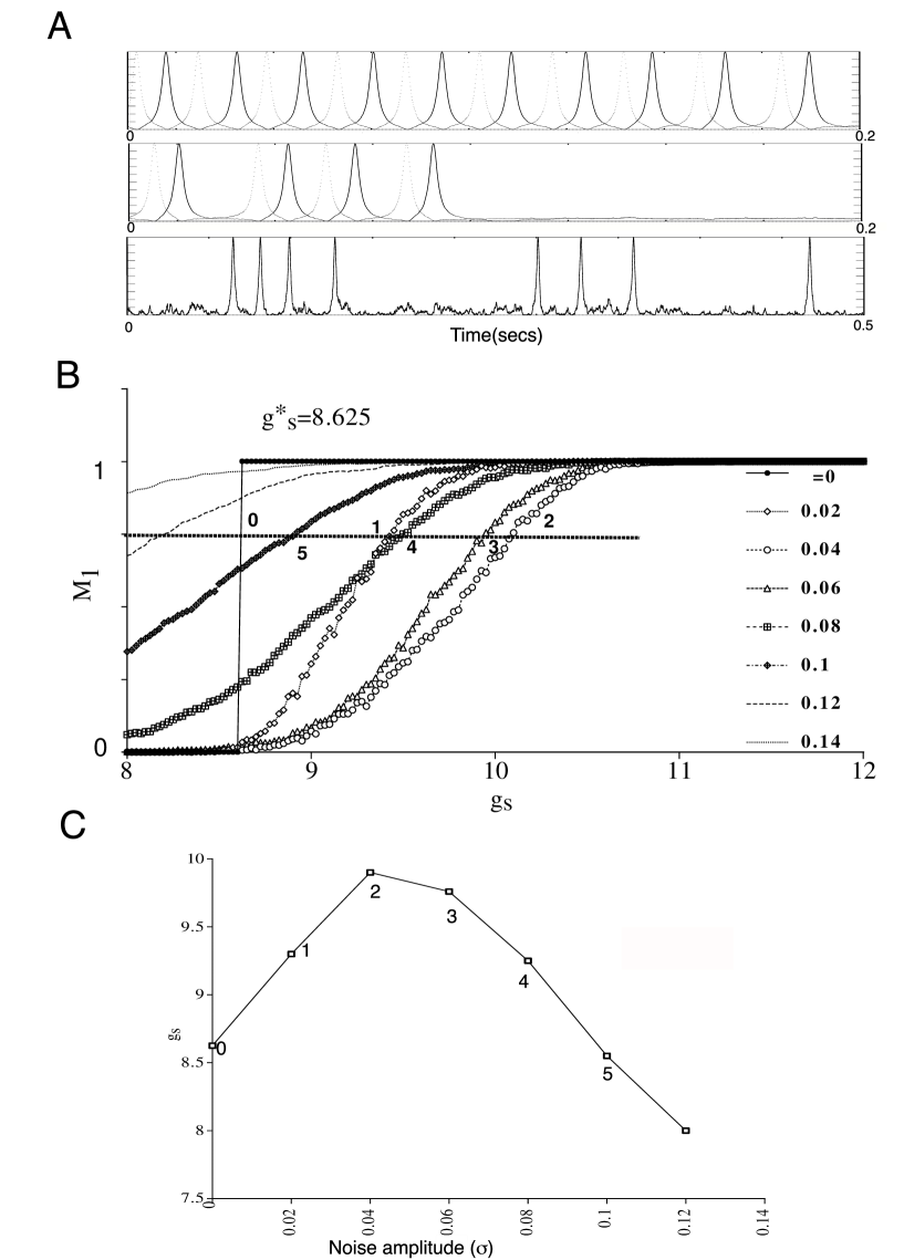
FIG. 1.: Asynchronous synaptically sustained oscillations in a positively coupled 2-cell circuit. A. Upper trace: the sustained firing in the noise free circuit. Middle trace: the sustained firing can be terminated by the action of small amplitude noise. Lower trace: larger amplitude noise induces an intermittent firing pattern. Here the noise injected into the two neurons is completely correlated, but the results are qualitatively identical for uncorrelated noises. B. Increasing noise delays sustained firing for low noise levels (traces 1,2) and advances firing for higher noise levels (traces 3,4,5), the horizontal dashed line and the numbers mark the test points $g_{s}^{2/3}$. C. Addition of noise has a non-linear effect on sustained firing in this coupled circuit. Here we plot the location of the test points $g^{2/3}_{s}$ See text for further details.

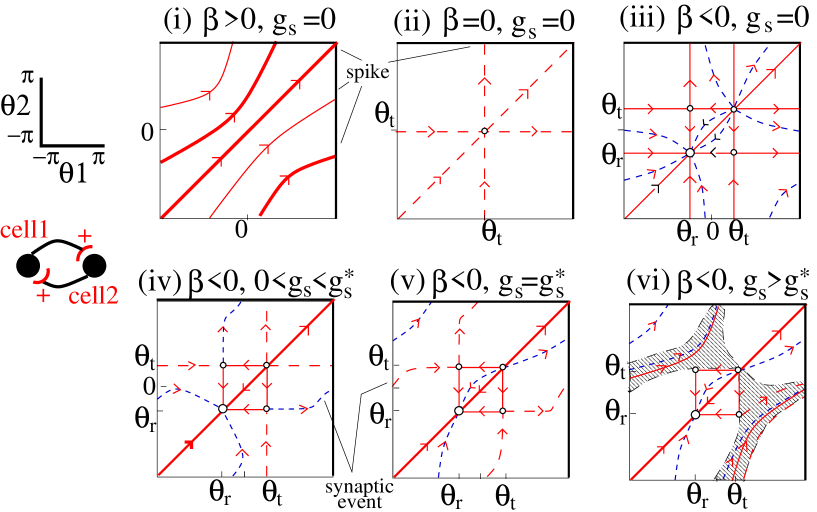
FIG. 2.: Different states of the network for various values of the intrinsic excitability of the cells, $\beta$, and the coupling strength, $g_{s}$. Axes plot the phase $(\theta_{1},\theta_{2})$ of each cell. See text for full details.

REFERENCES

- [1] J. P. Segundo, O.D. Martinez, K. Pakdaman, M. Stiber, and F. Vibert, J. Noise in sensory and synaptic coding - a survey of its history and a summary of its conclusions. Biophysical Journal, 66(2), 1994.
- [2] Z.F. Mainen and T.J. Sejnowski. Reliability of spike timing in neocortical neurons. Science, 268(5216):1503–1506, 1995.
- [3] J. J. Collins, C.C. Chow, and P. Grigg. Noise-mediated enhancements and decrements in human tactile sensation. Physical Review E, 56(1):923–926, 1997.
- [4] D.R. Chialvo, A. Longtin, and J. MullerGerking. Stochastic resonance in models of neuronal ensembles. Physical Review E., 55(2):1798–1808, 1997.
- [5] A. Longtin. Autonomous stochastic resonance in bursting neurons. Physical Review E., 55(1):868–786, 1997.
- [6] S. Lee, A. Neiman, and S. Kim. Coherence resonance in a Hodgkin-Huxley neuron. Physical Review E, 57(3):3292–3297, 1998.
- [7] R Rodriguez and H.C. Tuckwell. Noisy spiking neurons and networks: useful approximations for firing probabilities and global behavior. Biosystems, 48(1-3):187–194, 1998.
- [8] D.J. Mar, C.C. Chow, W. Gerstner, R.W. Adams, and J.J. Collins. Noise shaping in populations of coupled model neurons. Proc.Natl.Acad.Sci, USA, 96(18):10450–10455, 1999.
- [9] M. Usher, M. Stemmler, and Z. Olami. Dynamic pattern-formation leads to 1/f noise in neural populations. Physical Review Letters, 74(2):326–329, 1995.
- [10] D.S. Reich, J.D. Victor, B.W. Knight, T. Ozaki, and E. Kaplan. Response variability and timing precision of neuronal spike trains in vivo. Journal of Neurophysiology, 77:2836–2841, 1997.
- [11] R. Traub, M.A. Whittington, I.M. Standford, J.G.R. Jeffreys. A mechanism for generation of long-range oscillations in the cortex Nature, 282:621–624, 1996.
- [12] C. van Vreeswijk and H. Sompolinksy. Chaotic balanced state in a model of cortical circuits. Neural Computation, 10(6):1321–1371, 1998.
- [13] D. Golomb and Y. Amitai. Propagating neuronal discharges in neocortical slices: Computational and experimental study. Journal of Neurophysiology, 78(3):1199–1211, 1997.
- [14] J. J. Collins, T.T. Imhoff, and P. Grigg. Noise-enhanced tactile sensation. Nature, 383(6603):770, 1996.
- [15] W.J. Rappel and S.H. Strogatz. Stochastic resonance in an autonomous system with a nonuniform limit- cycle. Physical Review E, 50(4):3249–3250, 1994.
- [16] A. S. Pikovsky and J. Kurths. Coherence resonance in a noise-driven excitable system. Physical Review Letters, 78(5):775–778, 1997.
- [17] W. Maass. Networks of spiking neurons: The third generation of neural network models. Neural Networks, 10(9):1659–1671, 1997.
- [18] J.K. Lin, K. Pawelzik, U. Ernst, and T.J. Sejnowski. Irregular synchronous activity in stochastically-coupled networks of integrate-and-fire neurons. Network-Computation in Neural Systems, 9(3):333–344, 1998.
- [19] W. Maass. Bounds for the computational power and learning complexity of analog neural nets. SIAM Journal on Computing, 26(3):708–732, 1997.
- [20] G.B. Ermentrout. Type i membranes, phase resetting curves, and synchrony. Neural Computation, 8(5):979–1001, 1996.
- [21] B.S. Gutkin and B. Ermentrout. Dynamics of membrane excitability determine interspike interval variability: A link between spike generation mechanisms and cortical spike train statistics. Neural Computation, 10(5):1047–1065, 1998.