Measurement of persistence in 1-D diffusion

Abstract

Using a novel NMR scheme we observed persistence in 1-D gas diffusion. Analytical approximations and numerical simulations have indicated that for an initially random array of spins undergoing diffusion, the probability $p(t)$ that the average spin magnetization in a given region has not changed sign (i.e., “persists”) up to time $t$ follows a power law $t^{-\theta}$, where $\theta$ depends on the dimensionality of the system. Using laser-polarized ¹²⁹Xe gas, we prepared an initial “quasirandom” 1D array of spin magnetization and then monitored the ensemble’s evolution due to diffusion using real-time NMR imaging. Our measurements are consistent with analytical and numerical predictions of $\theta$ $\approx$ 0.12.

The dynamics of non-equilibrium systems is a field of great current interest, including such topics as phase ordering in binary alloys, uniaxial ferromagnets, and nematic liquid crystals, as well as coarsening of soap froth and diffusion of inhomogeneous fluids (e.g. [1]). The evolving spatio-temporal structures in these non-equilibrium systems depend crucially on the history of the system’s evolution and are not completely characterized by simple measures such as two-time correlation functions. Therefore, an important problem in the study of non-equilibrium dynamics is the development of simple and easily measurable quantities that give nontrivial information about the history of the system’s evolution. The recently identified phenomenon of “persistence” may be such a quantity: it characterizes the statistics of first passage events in spatially extended non-equilibrium systems [2, 3, 4, 5, 6, 7, 8, 9, 10, 11, 12, 13, 14, 15, 16, 17, 18, 19, 20, 21]. Persistence is being actively studied in statistical physics; e.g., in the search for universal behavior in non-equilibrium critical dynamics [9, 11, 18]. Practically, persistence may be important in determining what fraction of a system has reached a threshold condition as a function of time; e.g., in certain chemical reactions or disinfectant procedures.

Consider a non-equilibrium scalar field $\phi({\mathbf{x}},t)$ fluctuating in space and time according to some dynamics (e.g., a random array of interdiffusing spins). Persistence is the probability $p(t)$ that at a fixed point in space the quantity $[\phi({\mathbf{x}},t)-\langle\phi({\mathbf{x}},t)\rangle]$ has not changed sign up to time $t$. It has been found that this probability decays as a power law $p(t)\sim t^{-\theta}$, where the persistence exponent $\theta$ is generally nontrivial and has been suggested as a new universal dynamic critical exponent [9, 11]. This exponent depends both on the system dimensionality and the prevalent dynamics [7, 8], and is difficult to determine analytically due to the non-Markovian nature of the phenomena. Although $\theta$ has been calculated – largely using numerical techniques – for such systems as simple diffusion [7, 8, 13], the Ising model [4, 6, 15], and the more generalized $q$-state Potts model [2, 4, 5], few measurements of persistence have been performed (see Table I). In particular, “breath figures” [19], 2-D soap froth [20], and twisted nematic liquid crystals [21] are the only systems for which experimental results have been reported. Further experimental investigation is needed to probe the utility of persistence in studies of fundamental and applied non-equilibrium dynamics.

TABLE I.: A sample of reported persistence exponents. All values except those indicated are derived from numerical simulations; (^∗) denotes exact analytical results, (^†) experimental measurements, and (^‡) the result reported here.

Dim.	Diffusion	Ising	$\mathbf{q}$-Potts
1	0.12, 0.118‡	3/8∗, 0.35	$-\frac{1}{8}+\frac{2}{\pi^{2}}\left[\cos^{-1}\left(\frac{(2-q)}{\sqrt{2}q}\right)\right]^{2}$∗
2	0.19	0.22, 0.19†	0.86, 0.88† (large q)
3	0.24	0.26
refs	[7, 8, 13]	[4, 6] [21]†	[2, 4, 5] [20]†

In this paper we present the first measurement of persistence in a system undergoing diffusion (i.e., dynamics governed by Fick’s Law $\dot{\phi}=D\phi^{\prime\prime}$). Our experiment is also the first to observe persistence in one dimension (1-D). We employed a novel NMR technique to create an initial “quasi-random” spatial variation in the nuclear spin magnetization of a sample of laser-polarized ¹²⁹Xe gas. Subsequent 1-D NMR imaging allowed us to monitor the temporal evolution of the ensemble. We observed persistence by noting mean magnetization sign changes at fixed locations of constant size (i.e., imaging pixels) as a function of time. Using a simple theory (the “independent interval approximation”) and numerical simulations, both Derrida et al. [7] and Majumdar et al. [8] independently found that $\theta$ $\approx 0.121$ for 1-D diffusion. Newman and Toroczkai [13] found $\theta\approx$ 0.125 in 1-D using an analytic expression for the diffusion persistence exponent. Our measurements are consistent with these calculations.

Recently, laser-polarized noble gas NMR has found wide application in both the physical and biomedical sciences. Examples include fundamental symmetry tests [22], probing the structure of porous media [23], and imaging of the lung gas space [24]. These varied investigations, as well as the experiment reported here, exploit special features of laser-polarized noble gas: the large nuclear spin polarization ($\sim$ 10%) that can be achieved with optical pumping techniques; the long-lived nuclear spin polarization of the spin-1/2 noble gases ¹²⁹Xe and ³He; and rapid gas-phase diffusion.

We performed laser-polarization of xenon gas using spin-exchange optical pumping [25]. We filled a coated cylindrical glass cell [26] ($\sim$ 9 cm long, 2 cm I.D.) with approximately 3 bar of xenon gas isotopically enriched to 90% ¹²⁹Xe, 0.5 bar of N₂ gas, and a small amount of Rb metal. We heated the sealed cell to $\sim 100^{\circ}$C to create a significant Rb vapor. Optical pumping on the Rb D1 line was achieved with 15 W of circularly-polarized 795 nm light (FWHM $\sim$ 3 nm) from a fiber-coupled laser diode array. After 20 minutes the ¹²⁹Xe gas was routinely nuclear spin-polarized to 1% by spin-exchange collisions with the Rb vapor. We next cooled the cell to room temperature in a water bath and placed the cell inside a homemade RF solenoid coil (2.5 cm diameter, 15 cm long, $Q\sim$ 900) centered in a 4.7 T horizontal bore magnet (GE Omega/CSI spectrometer/imager) with ¹²⁹Xe Larmor frequency = 55.345 MHz. To allow the gas temperature to reach equilibrium, we left the cell in place for 20 minutes before starting the persistence measurements. At equilibrium under these conditions, the ¹²⁹Xe polarization decay time constant ($T_{1}$) was in excess of 3 hours, with a ¹²⁹Xe diffusion coefficient of 0.0198 cm²/s [27]. (Note that changes in the sample gas pressure, and hence the diffusion coefficient, simply cause a rescaling of the time variable and do not affect the persistence power law $p(t)\sim t^{-\theta}$ [8].)

The NMR pulse sequence we used to observe persistence in laser-polarized ¹²⁹Xe gas diffusion is shown schematically in Fig. 1. The first portion of the pulse sequence encodes a 1-D “quasi-random” pattern on the transverse magnetization of the laser-polarized ¹²⁹Xe gas sample by using $m$ pairs of variable-strength RF and magnetic-field-gradient pulses, repeated in rapid succession (see Fig. 1). Each pair of RF and gradient pulses adds different spatial Fourier components to the 1-D transverse magnetization pattern, with wavenumbers given by the gradient pulse area and Fourier component amplitudes set by the RF pulse area. Next, a $\pi/2$ RF pulse “stores” this quasi-random 1-D magnetization distribution along the longitudinal ($z$) direction while a subsequent strong (crusher) gradient pulse dephases any remaining transverse magnetization. The quasi-random longitudinal magnetization distribution then evolves with time due to diffusion and is monitored by a series of 1-D FLASH (Fast Low Angle SHot) NMR images [28, 29] (see Fig. 1).

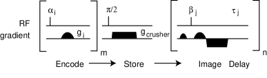
FIG. 1.: NMR pulse sequence used to encode a 1-D “quasi-random” pattern on the average magnetization of laser-polarized ¹²⁹Xe gas. Temporal evolution of the magnetization pattern is monitored with $n$ repetitions of a 1-D FLASH imaging routine [28]. For example, with $m=8$ encoding RF pulse/gradient pairs, the encoding pulse angles $\alpha_{i}$ = [30^∘, 35^∘, 37^∘, 41^∘, 45^∘, 50^∘, 63.5^∘, and 90^∘] while the encoding gradient amplitudes $g_{i}$ were chosen randomly. The imaging pulse angle $\beta_{j}$ was fixed at 8^∘ and the diffusion times $\tau_{j}$ were varied from 2.4 ms up to $\sim$ 2 s. The encoding gradients and the transverse magnetization dephasing “crusher” gradient were pulsed for 1 and 20 ms, respectively. Imaging gradients were applied for a total of 7.56 ms. The maximum gradient available was 6.7 G/cm.

The initial pattern of longitudinal ¹²⁹Xe magnetization is quasi-random in that there must be a minimum length scale to the induced variations in the ¹²⁹Xe magnetization, i.e., a maximum wavenumber in the pattern, for there to be sufficient NMR signal for useful imaging. (This minimum length scale was $\approx 0.6$  mm in our experiment.) Nevertheless, at longer length scales the induced pattern must be random enough that persistence behavior can be expected. Ideally, $\langle\phi(x,0)\phi(x^{\prime},0)\rangle=\delta(x-x^{\prime})$; however, calculations indicate that it is sufficient for the initial condition correlator to decrease faster than $|x-x^{\prime}|^{-1}$ for 1-D persistence [8]. We found that six to eight RF/gradient pulse pairs ($m=$ 6–8) were optimal for the desired quasi-random 1-D patterning of the ¹²⁹Xe magnetization. $m<6$ resulted in a pattern that was not sufficiently random, while $m>8$ significantly reduced the signal-to-noise ratio (SNR) of the NMR images. The requirement of $m\geq 6$ is supported by numerical calculations in which we modeled the NMR encoding sequence and simulated the subsequent gas diffusion using a finite difference first-order forward Euler scheme [7, 30]: we found persistence behavior (i.e., $p(t)\sim t^{-\theta}$) only when $m\geq 6$. The requirement of $m\leq 8$ was set by the available NMR signal (i.e., the finite ¹²⁹Xe magnetization), the necessity of rapid data acquisition to avoid excessive diffusion during the imaging sequence itself, the limitation of approximately 2$\pi\times$(0.6 mm)^-1 for the maximum wavenumber, and the maximum imaging gradient strength available.

For NMR imaging, we used a field of view (FOV) of 31.5 cm with 0.6 mm resolution, which thus divided the 9 cm cell into about 150 imaging pixels, each corresponding to a discernible spatial region of fixed size and location. We typically employed 8^∘ excitation RF pulse angles and acquired 32 1-D images spaced logarithmically in time from $\sim$ 3 ms to 5 s for a single experimental run. Longitudinal magnetization depletion due to imaging was highly uniform across the sample and did not affect the persistence measurement, since the relative magnetization amplitudes in neighboring imaging pixels was unchanged. An example of the images acquired in a typical run are shown in Fig. 2. For each pixel, we derived average magnetizations (aligned or anti-aligned to the main magnetic field) from the phase information contained in the time-domain NMR image data, and spatial positions from the frequency information [31]. An experimental run thus provided a record of the ¹²⁹Xe gas magnetization in each pixel as a function of time proceeding from the initial quasi-random pattern to the equilibrium condition of homogeneous (near-zero) polarization.

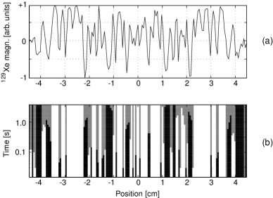
FIG. 2.: (a) Typical quasi-random initial pattern of ¹²⁹Xe magnetization resulting from 8 encoding RF pulse/gradient pairs. (b) 32 images of the evolving magnetization pattern were acquired at logarithmically increasing times. White (black) indicates average positive (negative) magnetizations for each of the 150 fixed-location imaging pixels of width $\approx$ 0.6 mm. Gray indicates pixels whose magnetization has changed sign at least once. The persistence exponent is determined from the growing fraction of gray pixels as a function of time.

To measure persistence, we noted the sign of the ¹²⁹Xe magnetization in each fixed spatial region (i.e., in each 1-D image pixel) and counted how many remained unchanged as a function of time. We equated the probability $p(t)$ with the fraction of pixels that had not changed sign up to time $t$. We chose $t=0$ to coincide with the first image and assigned the time index for each image to be the start time of the imaging RF pulse. Images with SNR $<40$ were excluded from the data to minimize uncertainty in pixel sign changes. We conducted about 30 experiments with image SNR $>40$, each with a unique set of randomly chosen encoding magnetic field gradients {$g_{i}$}. We observed that pixel sign changes occurred smoothly, so it was unlikely we missed sign changes with an error of more than one step in the imaging sequence. We employed two averaging schemes to combine the results from different experimental runs. In the first method, we used a linear least-squares fit of $\log[p(t)]$ vs. $\log[t]$ for each run, resulting in a distribution of power law exponents with a weighted mean $\theta$ $=0.119\pm 0.048$. With our numerical simulations of quasi-random initial conditions, we found that this averaging scheme results in a gaussian distribution of exponents with a mean value $\theta\approx$ 0.12 in agreement with previous calculations for 1-D diffusion [7, 8, 13] and our experimental results. In the second averaging scheme, we combined the data from all experimental runs; hence $p(t)$ represented the fraction of total pixels from all experiments that had not changed sign up to time $t$. We found $p(t)\sim t^{-\theta}$ with $\theta$ $=0.118\pm 0.008$ for 0.1 s $\leq t\leq$ 1 s. Figure 3 shows a log-log plot of $p(t)$ vs. $t$ when the data is averaged using this method.

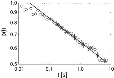
FIG. 3.: A log-log plot of $p(t)$, the fraction of regions (pixels) with ¹²⁹Xe spin magnetization that had not changed sign up to a time $t$, representing the sum of $\sim$ 30 different experimental runs. The solid line is a weighted linear least-squares fit to the data for $0.1$ s $\leq t\leq 1$ s, and yields $\theta=0.118\pm 0.008$. Error bars are derived from the number of pixels with amplitudes close to the image noise level and are shown when they exceed the plot symbol diameter.

The observed deviations from power law behavior for $t\lesssim 0.1$ s and $t\gtrsim 1$ s are explained by image resolution and finite size effects, respectively. At short times persistence is not observed because ¹²⁹Xe atoms have not yet diffused on average across a single 1-D image pixel ($\approx 0.6$ mm). The relevant diffusion time is $(0.6$ mm$)^{2}/(2D_{Xe})\approx 0.1$ s for our typical experimental conditions. At long times, the coarsening of the ¹²⁹Xe magnetization pattern by diffusion results in large “domains” of adjacent pixels with the same sign of the magnetization. Our simulations indicate that persistence is not observed when there are few domains in the finite size sample because the number of magnetization boundaries is greatly reduced; hence the rate of pixel sign-changing (i.e., the growth of the gray area in Fig. 2) is curtailed. Both the short and long-time deviations are seen in Fig. 4, where the average length $L$ of like-signed magnetization domains from all experimental runs is plotted against time. For $0.1$ s $\lesssim t\lesssim 1$ s, our data are in reasonable agreement with the expected power law $L\sim t^{1/2}$ for diffusion [1]. For $t\gtrsim 1$ s, we find $L\gtrsim 1$ cm, implying there are typically less than 10 magnetization boundaries in the 9 cm long sample cell.

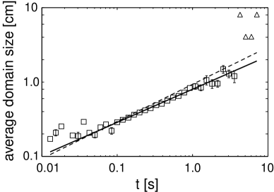
FIG. 4.: The average size $L$ of domains of adjacent pixels with uniform magnetization orientation, as a function of time $t$, derived from all experimental runs. For $0.1$ s $\leq t\leq 1$ s, $L\sim t^{\alpha}$ where $\alpha$ = $0.45\pm 0.02$ (solid line). The dotted line shows the expected $L\sim t^{1/2}$ behavior for an infinite system. The error in $L$ is shown where it exceeds the plot symbol size. The finite size limit on $L$ is evident in the four late-time points ($\triangle$), which were taken from the only two runs with sufficient SNR at long times.

In conclusion, we experimentally measured a persistence exponent $\theta$ $\approx$ 0.12 for 1-D diffusion, consistent with analytical and numerical studies. We performed the measurement using a novel NMR scheme with laser-polarized ¹²⁹Xe gas which allowed us to both encode a spatially “quasi-random” magnetization pattern and monitor its evolution over several seconds. We also observed the effect of finite sample size for long-time diffusion. In future work the experimental technique employed in this study may allow measurements of persistence in 2 and 3-D diffusion, in heterogeneous systems (e.g., porous media) infused with noble gas, and in ‘patterns’ [32].

The authors thank Satya Majumdar, Michael Crescimanno, and Lukasz Zielinski for useful discussions. This work was supported by NSF Grant No. CTS-9980194, NASA Grant No. NAG9-1166, and the Smithsonian Institution Scholarly Studies Program.

REFERENCES

- [1] A. J. Bray, Adv. Phys. 32, 357 (1994).
- [2] B. Derrida, A. Bray, and C. Godrèche, J. Phys. A. 27, L357 (1994).
- [3] A. Bray, B. Derrida, and C. Godrèche, Eur. Phys. Lett. 27, 175 (1994).
- [4] B. Derrida, V. Hakim, and V. Pasquier, Phys. Rev. Lett. 75, 751 (1995).
- [5] B. Derrida, P. M. C. de Oliveira, and D. Stauffer, Physica A 224, 604 (1996).
- [6] S. N. Majumdar and C. Sire, Phys. Rev. Lett. 77, 1420 (1996).
- [7] B. Derrida, V. Hakim, and R. Zeitak, Phys. Rev. Lett. 77, 2871 (1996).
- [8] S. N. Majumdar, C. Sire, A. J. Bray, and S. J. Cornell, Phys. Rev. Lett. 77, 2867 (1996).
- [9] S. N. Majumdar, A. Bray, S. Cornell, and C. Sire, Phys. Rev. Lett. 77, 3704 (1996).
- [10] J. Krug, H. Kallabis, S. N. Majumdar, S. J. Cornell, A. J. Bray, and C. Sire, Phys. Rev. E 56, 2702 (1997).
- [11] B. P. Lee and A. D. Rutenberg, Phys. Rev. Lett. 79, 4842 (1997).
- [12] S. N. Majumdar and A. J. Bray, Phys. Rev. Lett. 81, 2626 (1998).
- [13] T. J. Newman and Z. Toroczkai, Phys. Rev. E 58, R2685 (1998).
- [14] C. M. Newman and D. L. Stein, Phys. Rev. Lett. 82, 3944 (1999).
- [15] S. Jain, Phys. Rev. E 60, R2445 (1999).
- [16] C. Sire, S. N. Majumdar, and A. Rüdinger, Phys. Rev. E 60, 1258 (2000).
- [17] V. M. Kendon, M. E. Cates, and J.-C. Desplat, Phys. Rev. E 61, 4029 (2000).
- [18] A. J. Bray, Phys. Rev. E 62, 103 (2000).
- [19] M. Marcos-Martin, D. Beysens, J. P. Bouchaud, C. Godrèche, and I. Yekutieli, Physica A 214, 396 (1995).
- [20] W. Y. Tam, R. Zeitak, K. Y. Szeto, and J. Stavans, Phys. Rev. Lett. 78, 1588 (1997).
- [21] B. Yurke, A. N. Pargellis, S. N. Majumdar, and C. Sire, Phys. Rev. E 56, R40 (1997).
- [22] D. Bear, R. E. Stoner, R. L. Walsworth, V. A. Kostelecky, and C. D. Lane, Phys. Rev. Lett. 85, 5038 (2000).
- [23] R. W. Mair, G. P. Wong, D. Hoffmann, M. D. Hürlimann, S. Patz, L. M. Schwartz, and R. L. Walsworth, Phys. Rev. Lett. 83, 3324 (1999).
- [24] M. S. Albert, G. D. Cates, B. Driehuys, W. Happer, B. Saam, C. S. Springer, Jr., and A. Wishnia, Nature 370, 199 (1994).
- [25] T. G. Walker and W. Happer, Rev. Mod. Phys. 69, 629 (1997).
- [26] We used a wall coating of octadecyltrichlorosilane (OTS) to reduce Xe-wall interactions and hence increase longitundinal relaxation times.
- [27] R. W. Mair, D. G. Cory, S. Peled, C.-H. Tseng, S. Patz, and R. L. Walsworth, J. Mag. Res. 135, 478 (1998).
- [28] A. Haase, J. Frahm, D. Matthaei, W. Hänicke, and K.-D. Merboldt, J. Mag. Res. 67, 258 (1986).
- [29] A more detailed description of the NMR pulse sequence used in this experiment will be presented elsewhere.
- [30] W. H. Press, B. P. Flannery, S. A. Teukolsky, and W. T. Vetterling, Numerical Recipes in C (Cambridge University Press, Cambridge, U.K., 1988).
- [31] C. B. Ahn and Z. H. Cho, IEEE Trans. Med. Imag. MI-6, 32 (1987).
- [32] S. N. Majumdar, Curr. Sci. 77, 370 (1999).