Wave packet evolution approach to ionization of hydrogen molecular ion by fast electrons

Abstract

The multiply differential cross section of the ionization of hydrogen molecular ion by fast electron impact is calculated by a direct approach, which involves the reduction of the initial 6D Schrödinger equation to a 3D evolution problem followed by the modeling of the wave packet dynamics. This approach avoids the use of stationary Coulomb two-centre functions of the continuous spectrum of the ejected electron which demands cumbersome calculations. The results obtained, after verification of the procedure in the case atomic hydrogen, reveal interesting mechanisms in the case of small scattering angles.
PACS number(s): 34.80.Dp

I Introduction

New experimental methods, particularly, based on the multiple coincidence detection technique [1, 2, 3] stimulate the interest to fundamental theoretical studies of the dissociative ionization of diatomic molecules by electron impact. In this context the molecular hydrogen ion can be considered as the basic system in which the removal of the unique electron causes dissociation. Substantial theoretical analysis of the dissociative ionization of ${\rm H}^{+}_{2}$ by fast electrons was recently carried out in [4]. As mentioned in [4], the crucial point of calculating the cross-section of such processes is that no closed exact analytical wave functions of the continuum states exist. In [4] the final-state wave function of the ejected electron was found by taking a product of two approximate functions that take into account the two scattering centers. To improve the calculation it seems straightforward to obtain these functions with the exact numerical solutions of the two-center continuum problem. However, this approach involves a cumbersome procedure of calculating multi-dimensional integrals of the functions presented numerically that requires huge computer facilities and may cause additional computational problems. It seems reasonable to search for direct computational approaches, in which the basis of exact two-center continuum wave functions is not involved. Note that the potential advantage of such methods is that they could be generalized over a wider class of two-center systems starting from the molecular hydrogen ion as a test object. In the present paper we develop a direct approach to the ionization of hydrogen molecular ion by fast electrons that involves the reduction of the initial 6D Schrödinger equation to a 3D evolution problem followed by modeling of the wave packet dynamics.

Originally we intended to treat the incoming electron classically, its trajectory being approximated by a straight line with the deflection neglected. The bound electron was to be treated quantum mechanically. Preliminary calculations at the impact parameter $\rho=10$ a.u. has shown, first, that the probability of the emission of the electron having the energy of 50 eV is extremely small, and, second, that the direction of the electron emission is orthogonal to that of the incoming electron motion, that contradicts the results of [4]. This means that the main contribution to the small-angle scattering comes from the central collisions with the bound electron in the region of its localization. Generally, the classically estimated deflection angle of $1^{o}$ for scattered electron corresponds to the impact parameter of the order of 1 a.u., so that the trajectory passes through the molecule and the classical treatment of the incoming electron is not valid.

Here we develop and apply a direct approach to the calculation of the angular distribution of scattered and ejected electrons that involves the reduction of the initial 6D Schrödinger equation to a 3D evolution problem followed by modeling of the wave packet dynamics. The approach does not make use of the basis of stationary Coulomb two-center functions of the continuous spectrum for the ejected electron, whose proper choice is a crucial point of other model calculations. Our approach can be considered as the linearized version of the phase function method [5, 6] for the multi-dimensional scattering problem. The evolution problem is solved using the method based on the split-step technique [7] with complex scaling, recently proposed by some of us and tested in paraxial optics [8]. In the present paper the method as a whole is also tested using the well known problem of electron scattering by hydrogen atom [9].

II Basic equations

We start from the 6D stationary Schrödinger equation which describes two electrons in the field of two fixed protons

$$\left[H_{0}({\bf r})-\frac{1}{2}\nabla^{2}_{\bf R}+V({\bf r},{\bf R})\right]\Psi({\bf r},{\bf R})=E\Psi({\bf r},{\bf R}),$$ (1)

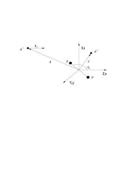
FIG. 1.: Coordinate frame

where ${\bf r}$ is the radius-vector of the electron initially bound in ${\rm H}_{2}^{+}$ and finally ejected, ${\bf R}$ is the radius-vector of the impact electron, $\hat{H}_{0}=-\frac{1}{2}\nabla^{2}_{\bf r}+U({\bf r})$ is Hamiltonian of ejected electron in the field of two protons, $V({\bf r},{\bf R})=U({\bf R})+U_{int}({\bf r},{\bf R})$ is the interaction between the impact electron and molecular ion, $U({\bf r})=-1/r_{1}-1/r_{2}$ is the attractive potential between the ejected (scattered) electron and the protons, $r_{1}=|{\bf r}-{\bf r}_{1p}|$, $r_{2}=|{\bf r}-{\bf r}_{2p}|$, ${\bf r}_{ip}$ is the radius-vector of the i-th proton, $U_{int}({\bf r},{\bf R})=1/|{\bf r}-{\bf R}|$ is the repulsive potential of interaction between the electrons. The origin of the coordinate frame is chosen in the center of symmetry of the molecular ion with the $Z$ axis directed along the momentum of the incident electron.

For the scattering problem solved here the energy of the system may be presented as $E=k_{i}^{2}/2+E_{0}$, where $-E_{0}$ is the ionization potential, $k_{i}$ is the momentum of the incident electron. Let us seek the solution of Eq.(1) in the form $\Psi({\bf r},X,Y,Z)=\psi({\bf r},{\bf R}_{\perp},Z)\exp(ik_{i}Z)$. Under the condition that $(k_{e}^{2}+k_{\perp}^{2}-2E_{0})/k_{i}^{2}<<1$ one can neglect the second derivative of $\psi$ with respect to $Z$. As a result we get the evolution-like equation for the envelope function $\psi({\bf r},{\bf R}_{\perp},Z)$

$$ik_{i}\frac{\partial\psi({\bf r},{\bf R}_{\perp},Z)}{\partial Z}=$$ (3)

$$\left\{\hat{H}_{0}({\bf r})-\frac{1}{2}\nabla^{2}_{{\bf R}_{\perp}}-E_{0}+V({\bf r},{\bf R})\right\}\psi({\bf r},{\bf R}_{\perp},Z).$$

Neglecting the large-angle scattering one can write the initial condition for $\psi$ as

$$\psi({\bf r},{\bf R}_{\perp},-\infty)=\psi_{0}({\bf r}).$$ (4)

To solve the 5D Schrödinger evolution equation(3) we use Fourier transformation with respect to the variable ${\bf R}_{\perp}$

$$\psi({\bf r},{\bf R}_{\perp},Z)=\frac{1}{2\pi}\int\psi_{{\bf k}_{\perp}}({\bf r},Z)\exp(i{\bf k}_{\perp}{\bf R}_{\perp})d{\bf R}_{\perp}.$$ (5)

Then Eq.(3) takes the form

$$ik_{i}\frac{\partial\psi_{{\bf k}_{\perp}}({\bf r},Z)}{\partial Z}=\left\{\hat{H}_{0}({\bf r})+\left(\frac{k_{\perp}^{2}}{2}-E_{0}\right)\right\}\psi_{{\bf k}_{\perp}}({\bf r},Z)$$ (6)

$$+\frac{1}{(2\pi)^{2}}\int V_{{\bf k}_{\perp}{\bf k}_{\perp}^{\prime}}({\bf r},Z)\psi_{{\bf k}_{\perp}^{\prime}}({\bf r},Z)d{\bf k}_{\perp}^{\prime},$$ (7)

where

$$V_{{\bf k}_{\perp}{\bf k}_{\perp}^{\prime}}({\bf r},Z)=\int\exp(-i({\bf k}_{\perp}-{\bf k}_{\perp}^{\prime}){\bf R}_{\perp})V({\bf r},{\bf R}_{\perp},Z)d{\bf R}_{\perp}$$ (8)

is the Fourier transform of the interaction potential $V({\bf r},{\bf R}_{\perp},Z)$.

Further simplification of the problem is possible if the amplitude of the incident wave is much greater than that of the scattered wave. In this case one can put

$$\psi_{{\bf k}_{\perp}}({\bf r},Z)=\delta({\bf k}_{\perp})\psi_{0}({\bf r})$$ (9)

in the integral term of Eq.(7). As a result we get the inhomogeneous equation

$$ik_{i}\frac{\partial\psi_{{\bf k}_{\perp}}({\bf r},Z)}{\partial Z} = \left\{\hat{H}_{0}({\bf r})+\left(\frac{k_{\perp}^{2}}{2}-E_{0}\right)\right\}\psi_{{\bf k}_{\perp}}({\bf r},Z)$$ (10)

$$+ \frac{1}{(2\pi)^{2}}V_{{\bf k}_{\perp}}({\bf r},Z)\psi_{0}({\bf r}),$$ (11)

where $V_{{\bf k}_{\perp}}({\bf r},Z)=V_{{\bf k}_{\perp}{\bf 0}}({\bf r},Z)$, with the initial condition $\psi_{{\bf k}_{\perp}}({\bf r},-\infty)=0$.

To calculate the integral with respect to transverse variables in the expression for $V_{{\bf k}_{\perp}}({\bf r},Z)$ it is easier to start from the known integral

$$\int\exp(-i{\bf k}{\bf R})\frac{1}{R}d{\bf R}=\frac{4\pi}{k^{2}}=\frac{4\pi}{k_{Z}^{2}+k_{\perp}^{2}}.$$ (12)

Carrying out the inverse Fourier transformation

$$\int_{-\infty}^{\infty}\exp(ik_{Z}Z)\frac{dk_{Z}}{k_{Z}^{2}+k_{\perp}^{2}}=\frac{\pi}{k_{\perp}}e^{-k_{\perp}|Z|},$$ (13)

one gets

$$V_{{\bf k}_{\perp}}({\bf r},Z)=\frac{2\pi}{k_{\perp}}e^{-k_{\perp}|Z-z|-i{\bf k}_{\perp}{\bf r}_{\perp}}$$ (15)

$$-\frac{2\pi}{k_{\perp}}\left[e^{-k_{\perp}|Z-d_{Z}|-i{\bf k}_{\perp}{\bf d}_{\perp}}+e^{-k_{\perp}|Z+d_{Z}|+i{\bf k}_{\perp}{\bf d}_{\perp}}\right].$$

Here $k_{\perp}=k_{i}\sin\theta_{s}$ is the transverse momentum component of the scattered electron, $\theta_{s}$ is the scattering angle, $\pm{\bf d}$ are the positions of the nuclei with respect to the center of symmetry. Note that terms in square brackets determine the elastic scattering of the incident electron by the nuclei.

Due to the exponential decrease of the source term with $|Z|$ the integration may be actually carried out within a certain finite interval $(-Z_{max},Z_{max})$. Hence the zero initial condition should be imposed at the point $-Z_{max}$.

Note that the approximation (9) is actually equivalent to the first Born approximation [9]. Multiply Eq.(11) by the complex conjugate function of the continuous spectrum of $\hat{H}_{0}$ and integrate over all ${\bf r}$. Then

$$ik_{i}\frac{dC_{{\bf k}_{\perp}}({\bf k}_{e},Z)}{dZ}=\left\{\frac{k_{e}^{2}}{2}+\frac{k_{\perp}^{2}}{2}-E_{0}\right\}C_{{\bf k}_{\perp}}({\bf k}_{e},Z)$$ (17)

$$+\frac{1}{(2\pi)^{2}}\int\psi^{*}({\bf k}_{e},{\bf r})V_{{\bf k}_{\perp}}({\bf r},Z)\psi_{0}({\bf r})d{\bf r},$$

where $C_{{\bf k}_{\perp}}({\bf k}_{e},Z)=\int\psi^{*}({\bf k}_{e},{\bf r})\psi_{{\bf k}_{\perp}}({\bf r},Z)d{\bf r}$ is the probability density amplitude for the transition of the initially bound electron into the state with the momentum ${\bf k}_{e}$. Let us substitute

$$C_{{\bf k}_{\perp}}({\bf k}_{e},Z)=\tilde{C}_{{\bf k}_{\perp}}({\bf k}_{e},Z)\exp(ik_{Z}Z),$$

where $k_{Z}$ is the increment of the longitudinal component of the momentum of the impact electron determined by the relation

$$k_{Z}=-\frac{1}{k_{i}}\left(\frac{k_{e}^{2}}{2}+\frac{k_{\perp}^{2}}{2}-E_{0}\right).$$ (18)

This relation is actually equivalent to the energy conservation law written neglecting the terms of the order of $k_{Z}^{2}$. The substitution yields

$$ik_{i}\frac{d\tilde{C}_{{\bf k}_{\perp}}({\bf k}_{e},Z)}{dZ}=$$ (20)

$$\frac{1}{(2\pi)^{2}}\exp(-ik_{Z}Z)\int\psi^{*}({\bf k}_{e},{\bf r})V_{{\bf k}_{\perp}}({\bf r},Z)\psi_{0}({\bf r})d{\bf r},$$

and

$$\tilde{C}_{{\bf k}_{\perp}}({\bf k}_{e},\infty)=$$ (22)

$$\frac{1}{ik_{i}(2\pi)^{2}}\langle e^{i{\bf k}_{s}{\bf R}}\psi({\bf k}_{e},{\bf r})|V({\bf r},{\bf R})|e^{i{\bf k}_{i}{\bf R}}\psi_{0}({\bf r})\rangle,$$

where ${\bf k}_{s}={\bf k}_{i}-{\bf K}$ is the momentum of the scattered electron, ${\bf K}=(-k_{X},-k_{Y},-k_{Z})$ is the momentum transfer.

Provided that the ejected electron has the momentum ${\bf k}_{e}$, the asymptotic form of the solution of Eq. (1) for the wave function of the scattered electron when $R\rightarrow\infty$ is

$$\Psi_{{\bf k}_{e}}^{as}({\bf R})=\exp(ik_{i}Z)+\frac{\exp(ik_{s}R)}{R}f_{{\bf k}_{e}}(\theta_{s},\phi_{s}).$$ (23)

The scattering differential cross-section(DCS) can be then expressed as

$$\sigma_{{\bf k}_{e}}(\theta_{s},\phi_{s})=\frac{k_{e}k_{s}}{k_{i}}\left|f_{{\bf k}_{e}}(\theta_{s},\phi_{s})\right|^{2},$$ (24)

On the other hand, the asymptotic form of the wave function resulting from the solution of Eq.(11) under the condition $Z\rightarrow\infty$ can be presented as

$$\Psi_{{\bf k}_{e}}^{as}({\bf R})=\exp(ik_{i}Z)+$$ (26)

$$\exp(ik_{i}Z)\int\tilde{C}_{{\bf k}_{\perp}}({\bf k}_{e},\infty)\exp(i{\bf k}_{\perp}{\bf R}_{\perp}+ik_{Z}Z)d{\bf k}_{\perp}.$$

Making use of the fact that the integrand has a stationary point we finally get

$$\Psi_{{\bf k}_{e}}^{as}({\bf R})=e^{ik_{i}Z}+$$ (28)

$$\frac{1}{Z}e^{i\left(k_{i}-\frac{k_{e}^{2}/2-E_{0}}{k_{i}}\right)Z+i\frac{k_{i}}{2Z}R_{\perp}^{2}}(-2\pi ik_{i})\tilde{C}_{{\bf k}_{\perp}^{0}}({\bf k}_{e},\infty),$$

where ${\bf k}_{\perp}^{0}=k_{i}\sin\theta_{s}(\cos\phi_{s},\sin\phi_{s})$, $R_{\perp}=R\sin\theta_{s}$, $Z=R\cos\theta_{s}$. The expression (28) agrees with (23) within the accuracy of the order of $\theta_{s}^{2}$ if we set

$$f_{{\bf k}_{e}}(\theta_{s},\phi_{s})=-2\pi ik_{i}\tilde{C}_{{\bf k}_{\perp}^{0}}({\bf k}_{e},\infty)$$ (30)

$$=-\frac{1}{2\pi}\langle e^{i{\bf k}_{s}{\bf R}}\psi({\bf k}_{e},{\bf r})|V({\bf r},{\bf R})|e^{i{\bf k}_{i}{\bf R}}\psi_{0}({\bf r})\rangle.$$

The latter expression is similar to the formula for $f_{{\bf k}_{e}}(\theta_{s},\phi_{s})$ derived in [9] using the first Born approximation.

III Calculation of the angular distribution

The asymptotic expression of the radial part of the wave function corresponding to the continuous spectrum of $\hat{H}_{0}$ can be written as

$$\psi^{as}_{E}(r,t)=\frac{1}{\sqrt{\upsilon(r)}\,\,r}\exp(-iEt+i\int^{r}\upsilon(r^{\prime})dr^{\prime})$$ (31)

where $t=Z/k_{i}$ is the evolution variable, $\upsilon(r)=\sqrt{2(E-U^{as}(r))}$, $E=\frac{k_{e}^{2}}{2}+\frac{k_{\perp}^{2}}{2}-E_{0}$, $U^{as}(r)=-Z^{\prime}/r$, $Z^{\prime}=2$ is charge of two protons. In the asymptotic limit one can take only the radial component of the momentum of the ejected electron into account. Then, according to [10], the expression for calculating the amplitude $A(k,\theta,\phi)$ takes the form

$$A_{{\bf k}_{\perp}}(k_{e},\theta_{e},\phi_{e})=$$ (33)

$$\frac{1}{\sqrt{2\pi}}\left.\int_{t_{0}}^{t_{1}}dt^{\prime}j(\psi_{{\bf k}_{\perp}}(r,\theta,\phi,t^{\prime}),\psi^{as}_{E}(r,t^{\prime}))\right|_{r=r_{max}},$$

where

$$j(\Psi,\Phi)=\frac{i}{2}\left\{\Psi\,r^{2}\frac{\partial\Phi^{*}}{\partial r}-\Phi^{*}\,r^{2}\frac{\partial\Psi}{\partial r}\right\},$$ (34)

is the flux introduced in [10], $t_{0}=-Z_{max}/k_{i}$ and $t_{1}>>Z_{max}/k_{i}$. The approximate relation (33) becomes exact when $t_{1}\rightarrow+\infty$ and simultaneously $r_{max}\rightarrow+\infty$.

The amplitudes defined by (33) are related with the coefficients introduced in Eq.(22) by

$$\left|A_{{\bf k}_{\perp}}(k_{e},\theta_{e},\phi_{e})\right|^{2}=k_{e}\left|\tilde{C}_{{\bf k}_{\perp}}({\bf k}_{e},\infty)\right|^{2}$$ (35)

Using (24),(30) and (35) we get the final expression for the differential cross-section

$$\sigma_{{\bf k}_{e}}(\theta_{s},\phi_{s})=(2\pi)^{2}k_{s}k_{i}\left|A_{{\bf k}_{\perp}}(k_{e},\theta_{e},\phi_{e})\right|^{2}.$$ (36)

In the region where $r>r_{max}$ we made use of the complex scaling technique [11] to suppress the non-physical reflection from the grid boundary.

IV Numerical scheme

The inhomogeneous Schrödinger equation to be solved can be written as

$$i\frac{\partial\Psi({\bf r},t)}{\partial t}=\hat{H}_{0}({\bf r})\Psi({\bf r},t)+F({\bf r},t),$$ (37)

The solution of Eq. (37) to within the second-order terms in $\Delta t$ can be expressed as the following sequence of equations:

$$\Psi^{0}_{l}\phantom{t+\Delta t)} = \Psi(t)-\frac{i\Delta t}{2}F({\bf r},t);$$ (38)

$$(1+i\frac{\Delta t}{2}\hat{H}_{0})\Psi^{1}_{l} = (1-i\frac{\Delta t}{2}\hat{H}_{0})\Psi^{0}_{l};$$ (39)

$$\Psi(t+\Delta t) = \Psi^{1}_{l}-\frac{i\Delta t}{2}F({\bf r},t+\Delta t).$$ (40)

The key step of the procedure is Eq.  (39) which defines nothing but Cranck-Nicholson scheme. To solve this equation we make use of the partial coordinate splitting (PCS). A finite-difference scheme is applied for the radial variable $r$ and the polar angle $\theta$. Fast Fourier transform (FFT) is used for the azimuthal angle $\phi$.

In the spherical coordinate system, the $z$-axis of which is directed along the symmetry axis of the molecule (and not along the velocity of the impact electron) and after the substitution $\Psi=\psi/r$ and the Fourier transformation of Eq.(39) the terms $\hat{H}_{0}\Psi^{0,1}_{l}$ entering this equation turn into

$$\hat{H}_{0}(r,\eta,m)\psi(r,\eta,m)=$$ (43)

$$-\frac{1}{2}\left[\frac{\partial^{2}}{\partial r^{2}}+\frac{1}{r^{2}}\left(\frac{\partial}{\partial\eta}(1-\eta^{2})\frac{\partial}{\partial\eta}-\frac{m^{2}}{1-\eta^{2}}\right)\right]\psi(r,\eta,m)$$

$$+U(r,\eta)\psi(r,\eta,m),$$

where $\eta=\cos\theta$, $m$ is the asimuthal quantum number.

Finite-difference approximation $\frac{\partial^{2}}{\partial r^{2}}\simeq D^{r}_{i_{2}i_{1}}$ and $\frac{\partial}{\partial\eta}(1-\eta^{2})\frac{\partial}{\partial\eta}-\frac{m^{2}}{1-\eta^{2}}\simeq D^{\eta,m}_{j_{2}j_{1}}$ of the differential operators entering Eq.(39) yields $M$ sets of linear equations, each set being of the order $L\times N$, where $M,\quad L$ and $N$ are the numbers of grid points in $\phi$, $\eta$ and $r$, respectively. Direct solution of each set of equations requires $NL^{2}$ operations at each step in $t$. The FFT that should be performed twice, first, when proceeding from (38) to (39), and second, from (39) to (40), requires $NLM\log_{2}M$ extra operations.

To reduce the number of operation we propose a double-cycle split-step scheme. In case when $\hat{H}_{0}$ can be presented as a sum $\hat{H}_{0}=\hat{H}_{1}+\hat{H}_{2}$, this scheme can be formulated as follows

$$\psi_{1} = \psi(t);$$ (44)

$$(I+i\frac{\Delta t}{4}\hat{H}_{1})\psi_{2} = (I-i\frac{\Delta t}{4}\hat{H}_{1})\psi_{1};$$ (45)

$$(I+i\frac{\Delta t}{4}\hat{H}_{2})\psi_{3} = (I-i\frac{\Delta t}{4}\hat{H}_{2})\psi_{2};$$ (46)

$$(I+i\frac{\Delta t}{4}\hat{H}_{2})\psi_{4} = (I-i\frac{\Delta t}{4}\hat{H}_{2})\psi_{3};$$ (47)

$$(I+i\frac{\Delta t}{4}\hat{H}_{1})\psi_{5} = (I-i\frac{\Delta t}{4}\hat{H}_{1})\psi_{4};$$ (48)

$$\psi(t+\Delta t) = \psi_{5},$$ (49)

which to within the second-order terms in $\Delta t$ corresponds to the initial Cranck-Nicholson scheme, $I$ and $H_{1,2}$ is square matrixes, $(I)_{i2i1j2j1}=\delta_{i2i1}\delta_{j2j1}$.

Now the problem is how to split the Hamiltonian $\hat{H}_{0}$ into two parts. Formal separation of radial and angular parts leads to difficulties associated with the singularity of the angular part. Due to this singularity the scheme appears to be conditionally stable with severe limitations imposed on the step $\Delta t$. Practically this version of the splitting scheme is applicable only if the grid in $r$ is rough enough.

To remove this limitation we propose a partial coordinate splitting scheme. Its principal idea is that in the vicinity of $r=0$ it is preferable not to split off the angular part at all. To implement this idea we introduce the $r$-dependent weight function $p(r)$ which is supposed to diminish in the vicinity of $r=0$ and define the discrete approximation of the operators $\hat{H}_{1,2}$ in the following way

$$(\hat{H}_{1}^{m})_{i_{2}i_{1}j_{2}j_{1}}=-\frac{1}{2}{\hat{D}^{r}}_{i_{2}i_{1}}\delta_{j_{2}j_{1}}+U^{as}(r_{i})$$ (51)

$$+p(r_{i_{1}})\left[-\frac{1}{2}\frac{{\hat{D}^{\eta,m}}_{j_{2}j_{1}}}{r_{i_{1}}^{2}}\delta_{i_{2}i_{1}}+U_{2}(r_{i_{1}},\eta_{j_{1}})\right];$$

$$(\hat{H}_{2}^{m})_{i_{2}i_{1}j_{2}j_{1}}=$$ (53)

$$(1-p(r_{i_{1}}))\left[-\frac{1}{2}\frac{{\hat{D}^{\eta,m}}_{j_{2}j_{1}}}{r_{i_{1}}^{2}}\delta_{i_{2}i_{1}}+U_{2}(r_{i_{1}},\eta_{j_{1}})\right],$$

here $U_{as}(r)+U_{2}(r,\eta)=U(r,\eta)$. It is reasonable to choose $p(r)$ as a cubic polynomial

$$p(r)=\left\{\begin{array}[]{ll}2\left[\frac{r-r_{a}}{a_{p}}\right]^{3}-3\left[\frac{r-r_{a}}{a_{p}}\right]^{2}+1,&r_{a}<r<r_{a}+a_{p};\\ 1,&r\leq r_{a};\\ 0,&r\geq r_{a}+a_{p};\end{array}\right.$$ (57)

where $r_{a}$ is the radius of the vicinity of $r=0$ where the splitting is absent, $a_{p}$ is the width of the area of partial splitting. Such a polynomial satisfies the condition of smooth connection at the boundaries that separate the region of partial splitting from the regions of full splitting, on one hand, and of no splitting at all, on another hand.

V Numerical calculations and results

The method was tested using the well-studied example of the impact ionization of atomic hydrogen. We compared our results with those given by the well-known expression obtained in the first Born approximation [12]. Good agreement was demonstrated in the energy interval of interest $E_{e}$ from 1 to 3 a.u., $E_{e}$ being the energy of the ejected electron.

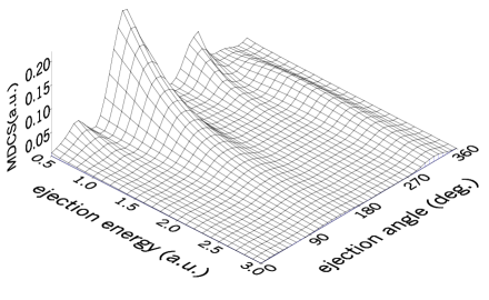
FIG. 2.: The multi-fold differential cross section (MDCS) of the ionization of $H_{2}^{+}$ versus the ejection angle $\theta_{e}$ and ejection energy $E_{e}$ for $\theta_{d}=135^{o}$

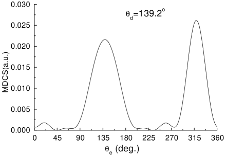
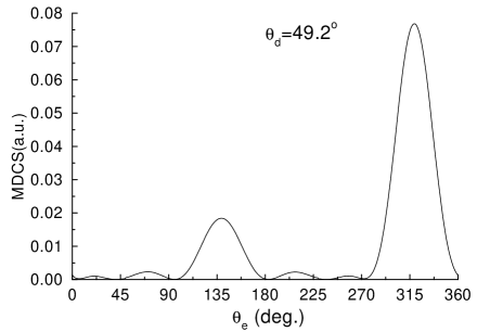
(a)

(b)

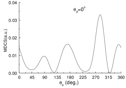
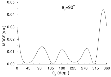
(c)

(d)

FIG. 3.: The multi-fold differential cross section (MDCS) of the ionization of $H_{2}^{+}$ versus the ejection angle $\theta_{e}$ for different angles $\theta_{d}$ : a)$\theta_{d}=139.2^{o}$ that corresponds to ${\bf d}\parallel{\bf K}$ ; b)$\theta_{d}=49.2^{o}$ that corresponds to ${\bf d}\perp{\bf K}$ ; c)$\theta_{d}=0^{o}$; d) $\theta_{d}=90^{o}$. The energy of the ejected electron $E_{e}=1.85$ a.u.=50.3 eV.

Our numerical studies concerning the molecular hydrogen ion focused on the variation of the multi-fold differential cross section (MDCS) concerning a coincidence detection of the two emerging electrons and one of the protons with the ejection angle $\theta_{e}$ at different orientations of the molecular axis, provided that the scattering angle is small. The examples of our results illustrated by Figs.2-5 are obtained under the following conditions: the momentum of the impact electron $k_{i}=$12.13 a.u. ($E_{i}\simeq 2000$ eV); the angle of scattering $\theta_{s}=1^{o}$. The impact and ejected electron trajectories and the molecular axis are supposed to lie in one plane. The latter restriction is not imposed by the method as such, it is just an example. Generally, one gets full information about the ejected electron, i.e., the dependence of MDCS from $E_{e}$, $\theta_{e}$ and $\phi_{e}$, after each run of the code at given values of the impact energy, scattering angle and molecular axis orientation. In Fig.2 demonstrates the energy-angle distribution, extracted from the data getting in result of one run of the code. In the planar geometry the orientation of the molecular ion is determined by a single angle $\theta_{d}$ between the impact direction and the internuclear axis. We remind that the momentum transfer vector was defined above as ${\bf K}={\bf k}_{i}-{\bf k}_{s}$. In Figs. 3 we present the particular cases of the dependence of MDCS upon $\theta_{e}$ when internuclear axis is a)parallel to the momentum transfer; b)perpendicular to the momentum transfer; c)parallel to the impact electron direction ${\bf k}_{i}$; d)perpendicular to the impact electron direction ${\bf k}_{i}$. As it could be expected basing on the elementary symmetry considerations, the first two plots are symmetric with respect to the direction of the momentum transfer that corresponds to the angle $\theta_{e}=319.2^{o}$. Since this symmetry is not assumed a priori in the procedure, this may be considered as one more evidence in favour of the validity of the results demonstrated.

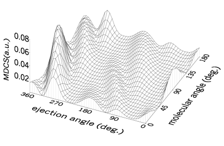
FIG. 4.: The multi-fold differential cross section (MDCS) of the ionization of $H_{2}^{+}$ versus the ejection angle $\theta_{e}$ and molecular angle $\theta_{d}$. The energy of the ejected electron $E_{e}=1.85$ a.u.=50.3 eV.

The recoil momentum ${\bf Q}_{recoil}={\bf K}-{\bf k}_{e}$ transmitted to the target has its minimum for ${\bf k}_{e}$ parallel to ${\bf K}$. In this case all the momentum is transferred to the ejected electron and the probability of the ionization is maximal. This is confirmed around $\theta_{e}=319.2^{o}$ on figures 3(a) and 3(b) where the inter-nuclear axis is respectively perpendicular and parallel to ${\bf K}$. So this is a good verification for our calculation. Now, for the situation where ${\bf k}_{e}$ is anti-parallel to ${\bf K}$, the recoil momentum $Q_{recoil}$ is maximal and the probability of the ionization is maximal. This is also visible for $\theta_{e}=139.2^{o}$. Now for the directions of the internuclear axis other than $\theta_{d}=139.2^{o}$ (where ${\bf d}$ is parallel to ${\bf K}$) or $\theta_{d}=49.2^{o}$ (where ${\bf d}$ is perpendicular to ${\bf K}$) the target does not respect the above analysis. This is due to the fact that the diatomic target behaves as an atomic target only for these two angles. The other situations present interference patterns the minima of which move when $\theta_{d}$ changes.

Fig.4 shows MDCS versus the ejection angle $\theta_{e}$ and internuclear angle $\theta_{d}$. As one can see, this dependence has rather a complex behaviour.

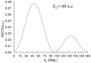
FIG. 5.: The multi-fold differential cross section of the ionization of $H_{2}^{+}$ as a function of the angle $\theta_{d}$ between the impact direction and the internuclear axis for fixed ejection angle $\theta_{e}=319.2^{o}$. The energy of the ejected electron is $E_{e}=1.85$ a.u.

To confirm the above dependence we show in Fig.5 a section of Fig.4 for fixed ejection angle $\theta_{e}=319.2^{o}$ which corresponds to the case when the ejected electron direction is parallel to the momentum transfer vector. It presents a variation of the MDCS with respect to the direction of the inter-nuclear axis. It can be clearly seen that the maximal value of MDCS is achieved when the internuclear axis is perpendicular to the momentum transfer direction that correspond to $\theta_{d}=49.2^{o}$. This result agrees with the hypothesis formulated in [13].

VI Conclusion

We have developed a procedure which determines the multiply differential cross section of the (e,2e) ionization of hydrogen molecular ion by fast electron impact, using a direct approach which reduces the problem to a 3D evolution problem solved numerically. Our method avoids the cumbersome stationary perturbative calculations, and opens the way for near future applications to the (e,2e) ionization of more complex atomic and molecular targets.

REFERENCES

• [1] Y.D. Wang, J.H. McGuire, and R.D. Rivarola, Phys. Rev. A 40, 3673 (1989).
• [2] S.E. Corchs, R.D. Rivarola, J.H. McGuire, and Y.D. Wang, Phys. Rev. A 47, 201 (1993).
• [3] S.E. Corchs, R.D. Rivarola, J.H. McGuire, and Y.D. Wang, Phys. Scr. 50, 469 (1994).
• [4] B. Joulakian, J. Hassen, R. Rivarola, and A. Motassim, Phys. Rev. A 54, 1473 (1996).
• [5] V.V. Babikov, Phase function method in quantum mechanics (Nauka, Moscow, 1968) (in Russian).
• [6] F. Calogero, Variable phase approach to potential scattering, (Academic, New York, 1967).
• [7] G.I. Marchuk, in Partial Differential Equation. II. SYNSPADE-1970 (Academic, New York, 1971).
• [8] V.V. Serov, A.I. Bychenkov, V.L. Derbov, and S.I. Vinitsky. Numerical scheme with external complex scaling for 2D Schrödinger equation in paraxial optics. Proc. SPIE 4002, 10 (1999).
• [9] N.F. Mott and H.S.W. Massey, The theory of atomic function, (Clarendon, Oxford, 1965).
• [10] A.M. Ermolaev, I.V. Puzynin, A.V. Selin, and S.I. Vinitsky, Phys. Rev. A 60, 4831 (1999).
• [11] C.W. McCurdy and C.K. Stroud, Computer Phys. Commun. 63, 323 (1991).
• [12] L.D. Landau and E.M. Lifshitz. Quantum Mechanics: Non-Relativistic Theory. (Pergamon, London, 1958), p. 458.
• [13] A. Bugacov, B. Piraux, M. Pont, and R. Shakeshaft, Phys. Rev. A 51, 4877 (1995).