Rotation in liquid ⁴He: Lessons from a toy model

Abstract

This paper presents an analysis of a model problem, consisting of two interacting rigid rings, for the rotation of molecules in liquid ⁴He. Due to Bose symmetry, the excitation of the rotor corresponding to a ring of N helium atoms is restricted to states with integer multiples of N quanta of angular momentum. This minimal model shares many of the same features of the rotational spectra that have been observed for molecules in nanodroplets of $\approx 10^{3}-10^{4}$ helium atoms. In particular, this model predicts, for the first time, the very large enhancement of the centrifugal distortion constants that have been observed experimentally. It also illustrates the different effects of increasing rotational velocity by increases in angular momentum quantum number or by increasing the rotational constant of the molecular rotor. It is found that fixed node, diffusion Monte Carlo and a hydrodynamic model provide upper and lower bounds on the size of the effective rotational constant of the molecular rotor when coupled to the helium.

The spectroscopy of atoms and molecules dissolved in helium nanodroplets is a topic of intense current interest [1, 2, 3]. One particular, almost unique feature of this spectroscopic host is that even heavy and very anisotropic molecules and complexes give spectra with rotationally resolved structure [4]. This spectral structure typically corresponds to thermal equilibrium, with $T\approx 0.38$ K, and has the same symmetry as that of the same species in the gas phase [5, 6]. The rotational constants, however, are generally reduced by a factor of up to four or five, while the centrifugal distortion constants are four orders of magnitude larger than for the gas phase [7, 6]. These large changes clearly reflect dynamical coupling between the molecular rotation and helium motion. At present, there are at least four different models proposed for the increased effective moments of inertia, at least two of which have reported quantitative agreement with experiment [8, 9, 10, 11]. The large observed distortion constants have not yet been quantitatively explained, and the most careful attempt to date to calculate them (for OCS in helium) gave an estimate $\approx 30$ times smaller than the experimental value [7]

The highly quantum many body dynamics of this condensed phase system has made it difficult to achieve a qualitative understanding of the observed effects. In cases like these, simple models can provide insight, especially if the lessons learned can be tested against more computationally demanding simulations that seek, however, to provide a first principles treatment of the properties of the system of interest. In this paper, one very simple model system will be explored that seeks to model the coupling of a molecular rotor to a first solvation shell of helium. The existing models for the reduced rotational constants agree that most of the observed effect comes from motion of helium in the first solvation shell. Some of the qualitative features of this model were discussed previously [7], but quanitative details were not persued in that work.

The ‘toy’ model considered consists of a planar rotor coupled to a symmetric planar ring of $N$ helium atoms. This model problem can be solved exactly, and can reproduce the size of the observed reductions in the rotational constant AND the size of the centrifugal distortion constants. This is the first time, to the authors knowledge, that the large effective distortion constants of molecules in liquid helium has been reproduced. Further, this model clearly resolves a confusion about the sign of the centrifugal distortion constant. Based upon the expected decreased following of the helium with increasing rotational angular velocity [12, 13], one can argue that the rotational spacing should increase faster than for a rigid rotor,i.e., that the effective centrifugal distortion constant should be negative, in conflict with experimental observations. The present model demonstrates, however, that opposite behavior is expected when the rotational velocity of the rotor is increased by increasing the rotational quantum number (where an increased angular anisotropy and following of the helium is predicted) or when the rotational constant of the isolated rotor is increased (where decreased angular anisotropy and following of the helium is predicted). The present model, therefore, rationalizes both the observed depenence of the increased moments of inertia on the rotational constant of the isolated molecule and the observed centrifugal distortion constants.

I The toy model

We will consider a highly abstracted model for rotation of a molecule in liquid helium. The molecule will be treated as a rigid, planar rotor with moment of inertia $I_{1}$. The orientation of the molecule is given by $\theta_{1}$ The liquid helium is treated as a ring of $N$ helium atoms that forms another rigid, planar rotor with moment of inertia $I_{2}$ and with orientation given by $\theta_{2}$. Because of the Bose symmetry of the helium, he helium rotor can only be excited to states with $N\hbar$ units of angular momentum. The lowest order symmetry allowed coupling between the molecule and the helium ring is given by a potential $V\cos\left[N(\theta_{1}-\theta_{2})\right]$. Any coupling spectral components that are not multiples of $N$ will lead to mixing of states that are not allowed by Bose symmetry, which is forbidden in quantum mechanics. The Hamiltonian is given by:

$$H=-\frac{\hbar^{2}}{2I_{1}}\frac{\partial^{2}}{\partial\theta_{1}^{2}}-\frac{\hbar^{2}}{2I_{2}}\frac{\partial^{2}}{\partial\theta_{2}^{2}}+V\cos N(\theta_{1}-\theta_{2})$$ (1)

We define $B_{1,2}=\frac{\hbar^{2}}{2I_{1,2}}$, the rotational constants for the uncoupled rotors. We can separate the above $H$ by introducing the two new coordinates:

$$\bar{\theta}=\frac{I_{1}\theta_{1}+I_{2}\theta_{2}}{I_{1}+I_{2}}\;\;\;\;\;\;\;\theta=\theta_{1}-\theta_{2}$$ (2)

in which we have:

$$H=H_{\rm r}+H_{\rm v}=-\frac{\hbar^{2}}{2(I_{1}+I_{2})}\frac{\partial^{2}}{\partial\bar{\theta_{1}}^{2}}+\left[-\frac{\hbar^{2}}{2}\left(\frac{1}{I_{1}}+\frac{1}{I_{2}}\right)\frac{\partial^{2}}{\partial\theta^{2}}+V\cos(N\theta)\right]$$ (3)

$\bar{\theta}$ is the variable conjugate to the total angular momentum; $\theta$ is a vibrational coordinate. We define $B_{\rm rigid}=\frac{\hbar^{2}}{2(I_{1}+I_{2})}$ and $B_{\rm rel}=\frac{\hbar^{2}}{2}\left(\frac{1}{I_{1}}+\frac{1}{I_{2}}\right)$. The eigenstates of $H$ separate into a product:

$$\psi(\bar{\theta},\theta)=e^{iJ\bar{\theta}}\psi_{\rm v}(\theta)$$ (4)

$J$ is the quantum number for total angular momentum. It would appear from the separable $H$ that the energy could be written as an uncoupled sum of a rigid rotor energy, $B_{\rm rigid}J^{2}$ ( not $J(J+1)$ because we have a planar rotor), and a ‘vibrational’ energy that is independent of $J$. However, the energies are not simply additive, due to the fact that the boundary condition for $\theta$ is $J$-dependent. When $\theta_{2}$ alone is changed by any multiple of $2\pi/N$, $\psi$ must be unchanged. However, a change of $-2\pi/N$ in $\theta_{2}$ results in a change of $-(2\pi/N)(I_{2}/(I_{1}+I_{2})$ in $\bar{\theta}$ and $+2\pi/N$ in $\theta$. Thus, the Bose symmetry of the helium ring is satisfied by taking as the boundary condition for $\psi_{\rm v}$:

$$\psi_{\rm v}\left(\theta+\frac{2\pi}{N}\right)=\exp\left(\frac{2\pi i}{N}\frac{I_{2}}{I_{1}+I_{2}}\,J\right)\,\psi_{\rm v}(\theta)$$ (5)

As a result, the ‘vibrational energies’ and eigenfunctions are a function of the total angular momentum quantum number, $J$. Note that the boundary condition is periodic in $J$, with period given by $N(I_{1}+I_{2})/I_{2}$.

The $J$ dependence of the boundary condition of the vibrational function is rather unfamiliar in molecular physics. This dependence can be removed by a Unitary transformation of the wavefunction:

$$\psi^{\prime}_{\rm v}(\theta)=\exp\left(-i\frac{I_{2}J}{I_{1}+I_{2}}\theta\right)\psi_{\rm v}(\theta)$$ (6)

The boundary condition on the transformed function is $\psi^{\prime}_{rmv}\left(\theta+\frac{2\pi}{N}\right)=\psi^{\prime}_{rmv}\left(\theta\right)$. The transformed hamiltonian, $H^{\prime}$, is given by:

$$H^{\prime}=\frac{1}{2I_{1}}\left(J-L\right)^{2}+\frac{1}{2I_{2}}L^{2}+V\cos\left(N\theta\right)$$ (7)

where $J=i\hbar\frac{\partial}{\partial\bar{\theta}}$ is the operator for total angular momentum, and $L=i\hbar\frac{\partial}{\partial\theta}$ is the angular momentum of the helium ring relative to a frame moving with the rotor. This form of the Hamiltonian closely resembles those widely used in treatment of weakly bound complexes [14]. Expansion of the $\left(J-L\right)^{2}$ gives a Coriolis term that couples the overall rotation to the vibrational motion, which makes the nonseperability of these motions evident. This form, however, hides the periodicity in $J$ of this the coupling.

We will now consider the two limiting cases. The first to consider is that where $|V|\gg N^{2}B_{\rm rel}$. In this case, the potential can be considered harmonic around $\theta=2\pi k/N,k=0\ldots N-1$ when $V$ is negative (and shifted by $\pi/N$ for $V$ positive) with harmonic frequency $\nu=\frac{1}{2\pi}\sqrt{2N^{2}|V|\left(\frac{1}{I_{1}}+\frac{1}{I_{2}}\right)}$. The wavefunction will decay to nearly zero at the maxima of the potential, and changes in the phase of the periodic boundary condition at this point (which happens with changes in $J$) will not significantly affect the energy. In this limit, the total energy is $E(J,{\rm v})=B_{\rm rigid}J^{2}+h\nu({\rm v}+1/2)$, and we have a rigid rotor spectrum with effective moment of inertia $I_{1}+I_{2}$. While there are $N$ equivalent minima, Bose symmetry assures that only one linear combination of the states localized in each well (the totally symmetric combination for $J=0$) is allowed, and thus there are no small tunneling splittings, even in the high barrier limit. The total angular momentum is partitioned between the two rotors in proportion to their moments of inertia, i.e. $<J_{1}>=\hbar J\cdot I_{1}/(I_{1}+I_{2})$ and $<J_{2}>=\hbar J\cdot I_{2}/(I_{1}+I_{2})$.

We will now consider the opposite, or uncoupled rotor, limit. The eigenenergies in this case are trivially $E(m_{1},m_{2})=B_{1}m_{1}^{2}+B_{2}m_{2}^{2}$ with eigenfunctions $\psi=\exp\left(im_{1}\theta_{1}+im_{2}\theta_{2}\right)$. $m_{1}$ can be any integer, while $m_{2}=Nk$, where $k$ is any integer. Introducing the total angular momentum quantum number $J=m_{1}+m_{2}$, we have $E(J,m_{2})=B_{1}(J-m_{2})^{2}+B_{2}\,m_{2}^{2}$. The lowest state for each $J$ has quantum numbers $m_{1}=J-Nk$ and $m_{2}=Nk$, where $k$ is the nearest integer to $B_{1}J/N(B_{1}+B_{2})$. Treating the quantum numbers as continuous, we have $E=B_{\rm rigid}J^{2}$, e.g., the same as for rigid rotation of the rotors. However when we restrict $J$ to integer values, for $J\leq N(B_{1}+B_{2})/(2B_{1})$, the energy spacing will be exactly that of a rigid rotor with rotational constant $B_{1}$. In general, as a function of $J$, the uncoupled ground state solutions follow the rigid rotor spectrum in $B_{1}$, but with a series of equally spaced curve crossings when the lowest energy $m_{2}$ value increases by $N$ as $J$ is increased by one quantum. These crossings allow the total energy to oscillate around that predicted for a rigid rotor with moment of inertia $I_{1}+I_{2}$.

II Numerical Results

Having handled the limiting cases, we can now turn our attention to the far more interesting question, which is how does the energy and eigenstate properties change as $V$ is continuously varied between these limits. We note that changing the sign of $V$ is equivalent to translation of the solution by $\Delta\theta=\pi$, and thus we will only consider positive values of $V$ explicitly. We also note that the eigenstates are not changed, and the eigenenergies scale linearly if $B_{1},B_{2}$, and $V$ are multiplied by a constant factor. As a result, we will take $B_{2}=1$ to normalize the energy scale. The solutions for finite values of $V$ were calculated using the uncoupled basis and the form of $H$ given in Eq. 1 with fixed values of $m_{1}+m_{2}=J$ and $m_{2}=Nk$. For each value of $J$, the matrix representation for $H$ is a tridiagonal matrix, with diagonal elements given by the energies for the uncoupled limit, and with off-diagonal elements given by $V/2$. Numerical calculations were done using a finite basis with $k=-15,-14,\ldots 15$.

Using $B_{1}=B_{2}$ and $N=8$, we have calculated the lowest eigenvalues of $H$ for $J=0,1,2$ and used these, by fitting to the expression $E({\rm v},J)=E_{0}({\rm v})+B_{\rm eff}J^{2}-D_{\rm eff}J^{4}$, to determine $B_{\rm eff}$ and $D_{\rm eff}$. Figure 1 shows the value of $B_{\rm eff}$ as a function of $V$ (both in units of $B_{2}$). It can be seen that $B_{\rm eff}$ varies smoothly from $B_{1}$ to $B_{\rm rigid}$ with increasing $V$, and is reaches a value half way between these limits for $V\approx N^{2}B_{2}$.

In order to rationalize this observation, we will now consider a Quantum Hydrodynamic treatment for the rotation [15]. Let the ground state density be $\rho(\theta)=|\psi_{\rm v}(\theta)|^{2}$. Now let the molecule classically rotate with angular velocity $\omega$. To first order in $\omega$, $\rho$ will not change (i.e. we will have adiabatic following of the helium density for classical infinitesimal rotation of the molecule). However, the vibrational wavefunction, $\psi_{\rm v}$ will no longer be real, but instead will have an angle-dependent phase factor whose gradient will give a hydrodynamic velocity. Solving the equation of continuity:

$$\frac{\rm d}{{\rm d}\theta}\left(\rho v\right)=-\frac{{\rm d}\rho}{{\rm d}t}=\omega r\frac{{\rm d}\rho}{{\rm d}\theta}$$ (8)

where $r$ is the radius of the helium ring, gives solutions of the form:

$$v(\theta)=\omega r\cdot\left(1-\frac{C}{\rho(\theta)}\right)$$ (9)

where $C$ is an integration constant. We determine $C$ by minimizing the kinetic energy averaged over $\theta$. This gives:

$$C=\frac{2\pi}{\int_{0}^{2\pi}\rho^{-1}}$$ (10)

and a kinetic energy:

$$\Delta E_{k}=\frac{1}{2}I_{2}\omega^{2}\cdot\left(1-\frac{4\pi^{2}}{\int_{0}^{2\pi}\rho^{-1}{\rm d}\theta}\right)$$ (11)

In the case of a uniform density, $\rho=(2\pi)^{-1}$ and $\Delta E_{k}=0$. As the density gets more anisotropic, the integral becomes larger and $\Delta E_{k}$ becomes larger, approaching the value for rigid rotation of the helium ring when $\rho$ has a node in its angular range. We define the hydrodynamic contribution to the increase in the moment of inertia of the heavy rotor due to partial rotation of the light rotor by $\Delta E_{k}=\frac{1}{2}\Delta I_{\rm h}\omega^{2}$. It is interesting to note that for the above lowest energy value of $C$, we have $\int_{0}^{2\pi}v(\theta){\rm d}\theta=0.$ (i.e. that the solution is ‘irrotational’) and that the net angular momentum induced in the helium is $\Delta I_{\rm h}\omega$. The lowest energy solution of the three dimensional Quantum hydrodynamic model satifies these conditions as well [10, 16].

The hydrodynamic model can be tested against the exact quantum solutions. Define $\Delta I_{\rm eff}$ as the effective moment of inertia for rotation (as calculated from $B_{\rm eff}$) minus the moment of inertia for the molecular rotor. $\Delta I_{\rm eff}$ will grow from $0$ for uncoupled rotors to $I_{2}$ as the coupling approachs the rigid coupling limit of high $V$. In the hydrodynamic model, $\Delta I_{\rm eff}=\Delta I_{\rm h}$. Figure 2 shows a plot that compares $\Delta I_{\rm eff}$ and $\Delta I_{\rm h}$ as a function of $V$. Each has been normalized by $I_{2}$. They are found to be in qualitative agreement for the full range of $V$, though the exact quantum solution is systematically below the hydrodynamic prediction. We note, however, that for the assumed parameters, the speed of the molecular rotor is equal to that of the helium rotor, while the hydrodynamic treatment assumed a classical, infinitesimal rotation of the molecular rotor.

The size of $\Delta I_{\rm eff}$ is determined by the degree of anisotropy of the ground state density in the vibrational displacement coordinate $\theta$. If $I_{1}$ is decreased at fixed $I_{2}$ and $V$, the effective mass for $\theta$, which is $(I_{1}^{-1}+I_{2}^{-1})^{-1}$ will also decrease, which will decrease the anisotropy produced by $V$. Fig 3 shows how the normalized $\Delta I_{\rm eff}$ and $\Delta I_{\rm h}$ vary as the molecular rotational constant, $B_{1}$, changes from $0$ to $2B_{2}$. This calculation was done for $V=100$, close to the value corresponding to maximum difference of $\Delta I_{\rm eff}$ and $\Delta I_{\rm h}$ for $B_{1}=B_{2}$. This plot demonstrates that the hydrodynamic prediction becomes exact in the limit that $B_{1}\rightarrow 0$, i.e., in the case that the assumption of infinitesimal rotational velocity of the molecule holds. However, it substantially overestimates the increase effective moment of inertia when $B_{1}\geq B_{2}$. This decrease in the increase moment of inertia with increasing rotational constant of the heavy rotor is the effect previously interpreted as the breakdown of adiabatic following in the literature on the rotational spectrum of molecules in liquid Helium [12, 10, 13].

Figure 4 shows a plot of $D_{\rm eff}$ as a function of $V$ for $B_{1}=B_{2}=1$. $D_{\rm eff}=0$ is zero in both limits, and has a maximum value near the value of $V$ at which $B_{\rm eff}$ is changing most rapidly. It is interesting to explicitly point out that this $D_{\rm eff}$ value arises entirely from changes in the angular anisotropy of the helium density with $J$, as the model does not allow for an increase in the radial distance of the helium, which has previously been considered [7]. Further, the peak value of $D_{\rm eff}\approx 1.8\,\cdot 10^{-3}B_{1}$ is in remarkably good agreement with the ratio of $D_{\rm eff}$ to the gas phase molecular rotational constant observed for a number of molecules in liquid helium. For example, for OCS this ratio is found to be $2\cdot 10^{-3}$ [7], while for HCCCN, the same ratio was found to be $1\cdot 10^{-3}$ [17].

We can gain further insight by examining the rotational energy systematically as a function of $J$. Figure 5 shows the rotational excitation energy ($E(0,J)-E(0,0)$) divided by $J^{2}$ as a function of $J$. The calculations were done with $V=100$. The rotational excitation energy approaches that of the $B_{\rm rigid}J^{2}$ for high $J$. Further, it reaches this value for $J$ equal to multiples of $N(I_{1}+I_{2})/I_{2}$, which matches the periodicity of the boundary conditions for $\psi_{\rm v}$. $J$ values that lead to the same boundary conditions for $\psi_{\rm v}$ will differ in energy only by the eigenvalues of $H_{\rm r}$, and thus it follows from Eq. 2, that of a rigid rotor with rotational constant $B_{\rm rigid}$. For the first half of each period in $J$, $\psi_{\rm v}$ is found to increase in its anisotropy, and therefore the energy increases, as $J$ is increased (See Fig. 6). This can be understood when one considers the fact that for $J=N(I_{1}+I_{2})/(2I_{2})$, the boundary condition is that $\psi_{\rm v}(2\pi/N)=-\psi_{\rm v}(0)$, i.e. the wavefunction will be real but have $N$ nodes in the interval $[0,2\pi]$.

Classically, the molecular rotor is characterized by its rotational angular velocity, $\omega=2B_{1}J$. However, we see that the quantum treatment of the two coupled rotors gives opposite results when $\omega$ is increased by increasing either $B_{1}$ or $J$. For increases in $B_{1}$, the ‘degree of following’ of the light rotor decreases for fixed potential coupling, as seems intuitively reasonable. However, for increases in $J$, the anisotropy of the potential and thus the ‘degree of following’ initially increases, and thus so does the effective moment of inertia of the coupled system. This behavior continues until one passes through a resonance condition where the helium can be excited by transfer of $N$ quantum of angular momentum from molecular rotor to the helium. This resonance condition is missing from the classical treatment of the coupling between the rotors, where the angular velocity of the molecular rotor is treated as a fixed quantity, $\omega$, which is one of the parameters of the problem.

III Nodal Properties of Solutions

It is possible to calculate the rotational excitation energies of clusters of helium around a molecule by use of the Fixed Frame Diffusion Monte Carlo (FFDMC) method [12]. As in most DMC methods, this method should yield (except for statistical fluctuations) a upper bound on the true energy, finding the optimal wavefunction consistent with the nodal properties that are imposed on the wavefunction by construction. In the case of FFDMC, the nodal planes are determined by the free rotor rotational wavefunction for the molecule alone, i.e. that the sign of the wavefunction (which is taken to be real) for any point in configuration space is the same as that of the rotor wavefunction at the same Euler angles.

We can examine the exact solutions of our toy problem to gain insight into the accuracy of the nodal planes assumed in FFDMC. The wavefunctions we have considered up to now are complex, but because of time reversal symmetry, the solutions with $J$ and $-J$ rotational quantum numbers must be degenerate. Symmetric combination of these solutions just gives the Real part of $J$ solution, and the antisymmetric combination the Imaginary part. The real part is given by:

$$\psi^{\rm R}_{J}(\theta_{1},\theta_{2})=\cos(J\theta_{1})Re(\psi^{\prime}(\theta_{2}-\theta_{1}))-\sin(J\theta_{2})Im(\psi^{\prime}(\theta_{2}-\theta_{1}))$$ (12)

where

$$\psi^{\prime}(\Delta\theta)=\sum_{k}c^{J}_{k}\exp(ikN\Delta\theta)$$ (13)

and $c^{J}_{k}$ are the eigenvector coefficients obtained from diagonalization of the real Hamiltonian matrix in the uncoupled basis. Examination of the numerical solutions reveals that for $J<N$, $Re(\psi^{\prime})$ has no nodes, while $Im(\psi^{\prime})$ has nodes at $\Delta\theta$ equal to integer multiples of $\pi/N$. Thus, if $Im(\psi^{\prime})=0$, then the solution would satisfy the FFDMC nodal properties exactly. However, for finite $Im(\psi^{\prime})$, the nodal surfaces, rather than being on the planes $\theta_{1}=$ constant, are modulated N times per cycle along the $\theta_{1}=$ constant line. For $V=80$ and $B_{1}=B_{2}=1$, the maximum value of $Im(\psi^{\prime})$ is about $4\%$ of $Re(\psi^{\prime})$, and growing approximately linearly for low $J$.

In order to test the quantiative implications of this error in the nodal properties, importance sampled DMC calculations have been done for the present two rotor problem. The explicit DMC algorithm given by Reynolds et al. [18] was used with minor change [19]. The guiding function, $\psi_{\rm T}$, which determines the nodes, was selected as $\cos(J\theta_{1})\psi_{\rm v}^{0}(\theta_{1}-\theta_{2})$, where $\psi_{\rm v}^{0}$ is the real, positive definite eigenstate for the $J=0$ problem. The rotational constant, $B_{\rm DMC}$ is defined as the DMC estimated energy for $J=1$ less the exact ground state eigenenergy for $J=0$, and will be (except for sampling and finite time step bias) an upper bound on the true $B$ value calculated earlier. The points plotted in figure 1 are the calculated values of $B_{\rm DMC}$ with the estimated $2\sigma$ error estimates. It is seen that the fixed node DMC estimates of $B_{\rm eff}$ are excellent for low values of $V$, but underestimate the contribution of the Helium ring to the effective moment of inertia as it is coupled more strongly to the rotor.

IV Relationship with a more Realistic Model

In a series of insightful lectures, Anthony Leggett analyzed the properties of the ground state of $N$ Helium atoms confined to an annulus of radius $R$ and spacing $d\ll R$ [15]. The walls of the annulus are allowed to classically rotate with angular velocity $\omega$. While not stated explicitly, the walls of the annulus couple to the helium via a time dependent potential, which is static in the rotating frame. As such, our rotating diatomic molecule can be considered as a special case of the problem treated by Leggett. If one transforms to the rotating frame, the quantum hamiltonian is the same as for the static ($\omega=0$) problem. However, the boundary condition for the wavefunction in this frame is given by [15][Eq. (2.10)]:

$$\Psi^{\prime}_{0}(\theta_{1},\theta_{2}\ldots\theta_{j}+2\pi\ldots\theta_{N})=\exp\left(2\pi imR^{2}\omega/\hbar\right)\Psi^{\prime}_{0}(\theta_{1},\theta_{2}\ldots\theta_{j}\ldots\theta_{N})$$ (14)

In making a comparison to the results of the toy model, we note that for this system $I_{2}=NmR^{2}$ (the classical moment of inertia for the helium) and $J=\omega(I_{1}+I_{2})/\hbar$. Substitution shows that the phase factor in Eq. 14 is identical to that derived above for Eq. 5. Note, however, that Eq. 14 refers to moving one helium atom by $2\pi$, while Eq. 5 refers to motion of all $N$ helium atoms by $2\pi/N$. Motion of all $N$ helium atoms by $2\pi$ will result in a phase factor of $2\pi iNmR^{2}\omega/\hbar=2\pi iI_{2}J/(I_{1}+I_{2})$ in both treatments.

Leggett considered the change in helium energy produced by rotation of the walls. Let $E_{0}$ be the ground state energy for the static problem, and $E^{\prime}_{0}(\omega)$ the ground state energy in the rotating frame. The ground state energy in the laboratory frame is given by [15][Eq. (2.12)]:

$$E_{\rm lab}=E_{0}+\frac{1}{2}I_{2}\omega^{2}-\left[E^{\prime}_{0}(\omega)-E_{0}\right]$$ (15)

For the ground state of Bosons, we further have that $E^{\prime}_{0}(\omega)\geq E_{0}$, with equality only when $\omega$ equals integer multiples of $\omega_{0}=\hbar/mR^{2}$ since the nodeless state has the lowest possible energy. At $\omega=k\omega_{0}$, the helium rigidly rotates with the walls. This agrees exactly with the numerical results of the toy model, as shown in Figure 5. In making comparisons with this model, one should remember that $E_{\rm lab}$ does not include the kinetic energy of the walls (rotor). Thus the more general treatment of Leggett supports one of the central insights of the toy model, that the large effective distortion constants for molecular rotors in helium is a consequence of an increased helium following of the rotor with increasing angular velocity, which in turn is a direct consequence of the $\omega$ dependence of the single-valuedness boundary condition in the rotating frame.

The moment of inertia for the ground state of the helium can be defined by:

$$I=\left(\frac{d^{2}E_{\rm lab}}{d\omega^{2}}\right)_{\omega\rightarrow 0}=I_{2}-\left(\frac{d^{2}E^{\prime}_{0}(\omega)}{d\omega^{2}}\right)_{\omega\rightarrow 0}$$ (16)

Leggett defined the “normal fraction” of the helium by the ratio $I/I_{2}$, which is equal to unity if $E^{\prime}_{0}(\omega)$ is independent of $\omega$ as $\omega\rightarrow 0$. This will occur if the wavefunction has ‘nontrivial’ nodal planes, since the phase of the wavefunction can be changed discontinuously at a node without cost of energy. Nodal plans associated with overlap of particles, however, are ‘trivial’ in that the phase relationship on each side of the node is determined by the exchange symmetry of the wavefunction, and thus cannot be used to match the boundary conditions without extra cost of energy. In our toy problem, when $V$ is very large, the vibrational wavefunction becomes localized, introducing near nodes at the maxima of the potential, and as a result the ground state is described by a near unity normal fraction; we have what Leggett refers to as a ‘normal solid’. Conversely, as the uncoupled limit is approached, the helium ring does not contribute to the kinetic energy of the lowest rotational states and we have $I\rightarrow 0$, and we have zero normal fraction (i.e. the helium has unity superfluid fraction). Following Leggett’s definition, one finds that the normal fraction is given by $\Delta I_{\rm eff}/I_{2}$. Thus, Figure 2 can thus be interpreted as the normal fluid fraction for the ground state as a function of the strength of the potential coupling. Leggett’s analysis is based upon a classical treatment of the motion of the walls, which implies $I_{1}\gg I_{2}$, in which limit the hydrodynamic model exactly predicts the normal fluid fraction.

V Acknowledgement

This work was supported by the National Science Foundation and the Air Force Office of Scientific Research.

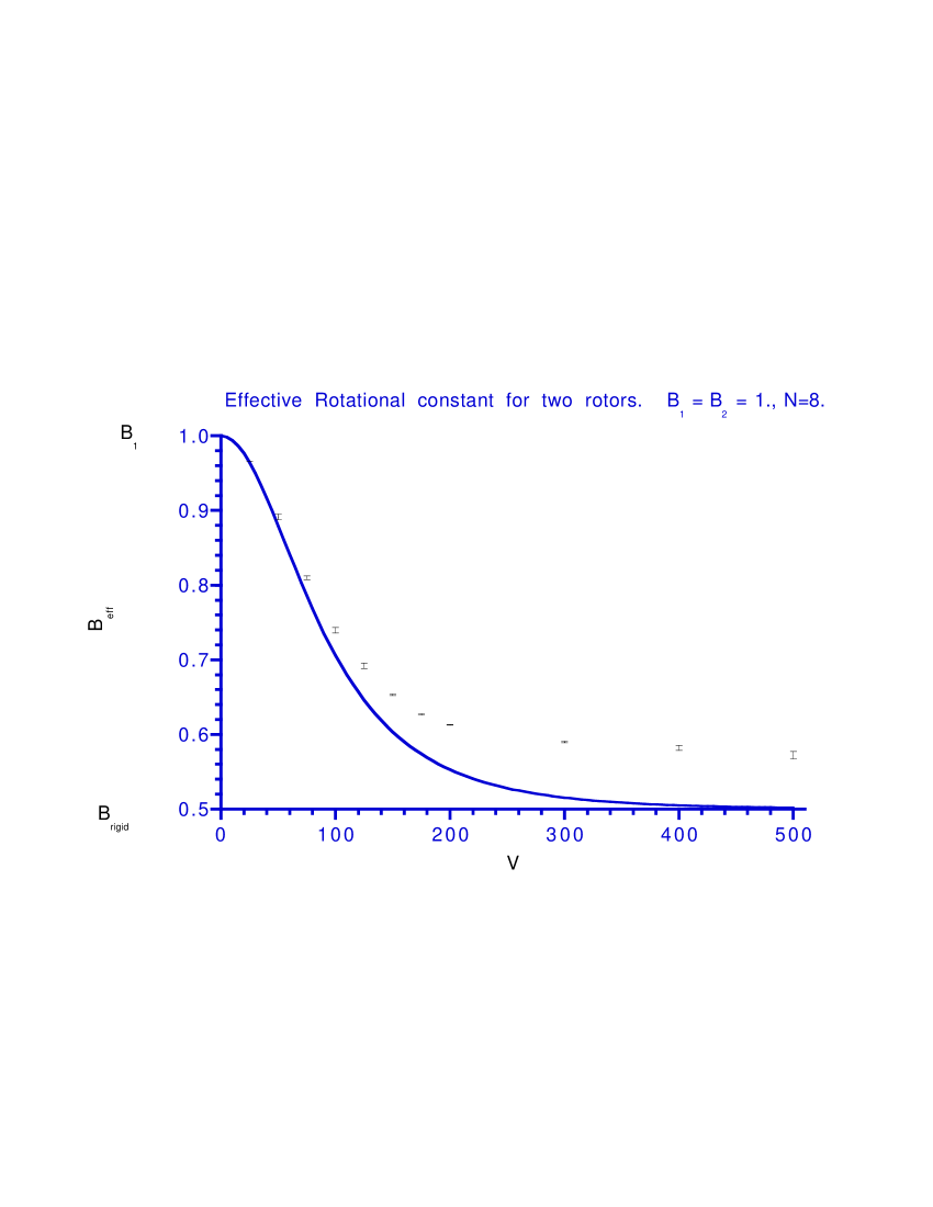
FIG. 1.: Effective Rotational Constant for two coupled rotors as a function of the interaction potential strength. $B_{1}=B_{2}=1$, and the second rotor can only be excited to states with multiples of 8 quanta. The individual points are the $B$ effective values calclated by a fixed node, Diffusion Monte Carlo calculation. The error bars on these points are the estimated $2\sigma$ sampling error.

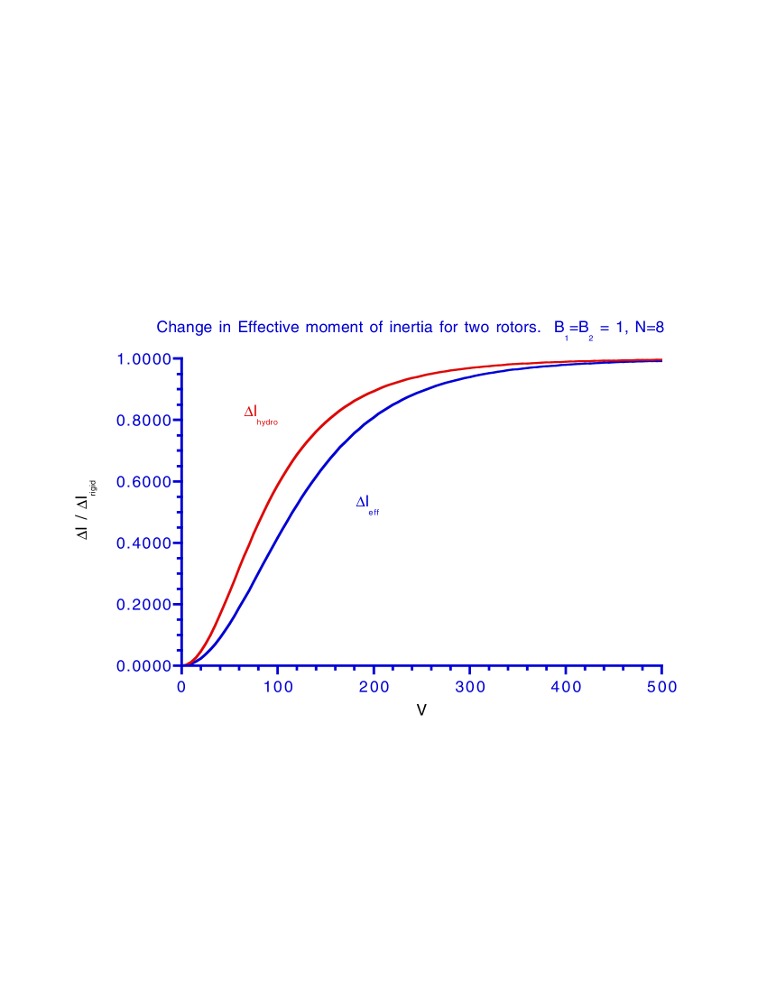
FIG. 2.: Increase in effective moment of inertia of molecule, $\Delta_{\rm eff}$ due to coupling to rotor made of 8 helium atoms. $\Delta I_{\rm hydro}$ is the same quantity estimated by the hydrodynamic model. Both are calculated as a function of the potential coupling strength, and the results normalized to the rigid rotor moment of inertia of the 8 helium rotor

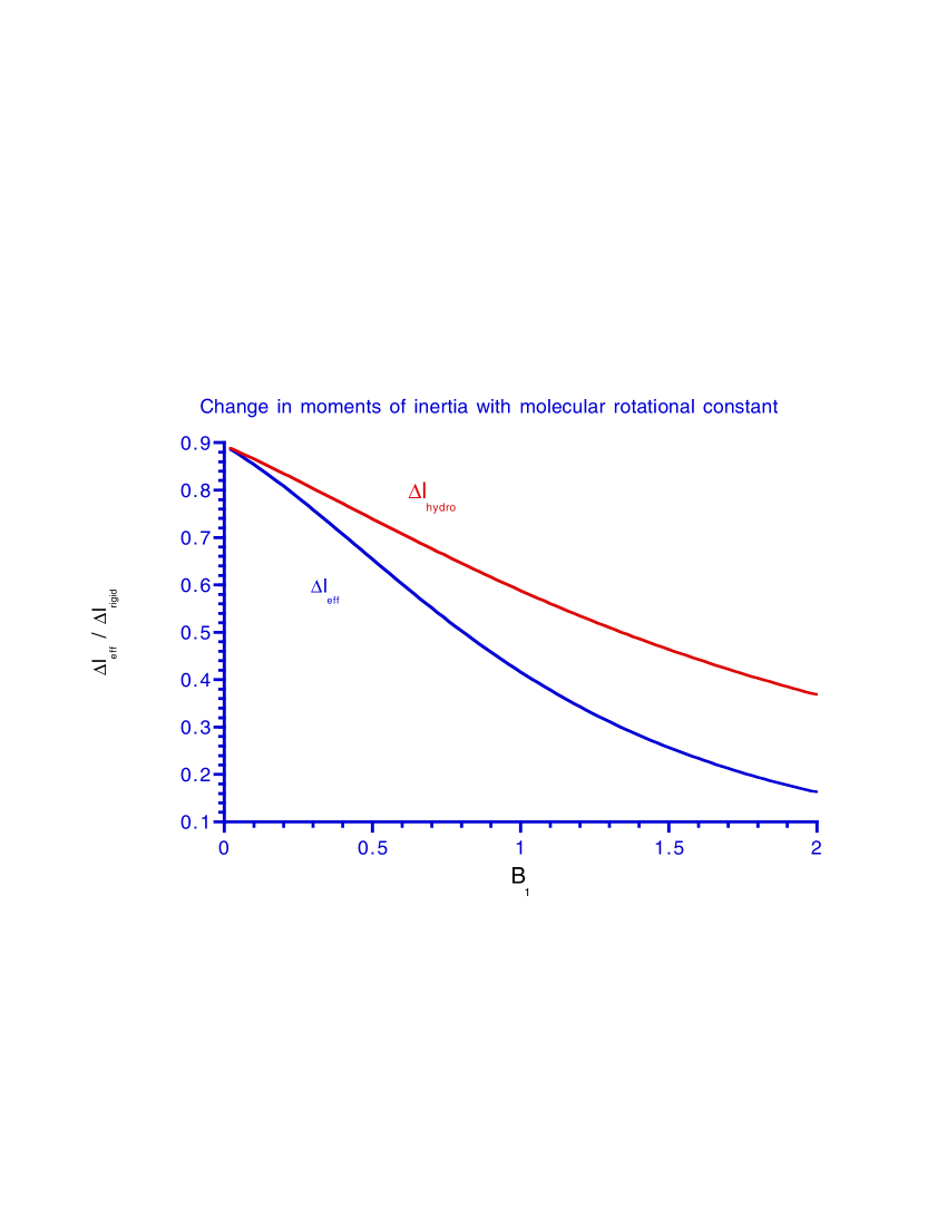
FIG. 3.: Same as Figure 2, except as a function of the rotational constant of the molecule, normalized to the rotational constant of the 8 helium rotor.

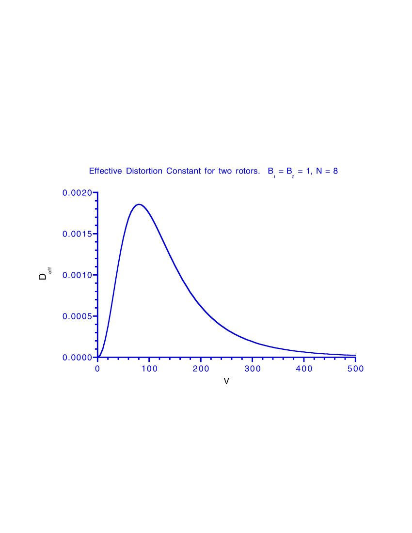
FIG. 4.: The effective centrifugal distortion constant, $D_{\rm eff}$, for molecule coupled to ring of 8 helium atoms as a function of the strength of the coupling, $V$. Both $D_{\rm eff}$ and $V$ are normalized to the rotational constants of the molecule and 8 helium rotor, which are taken as equal.

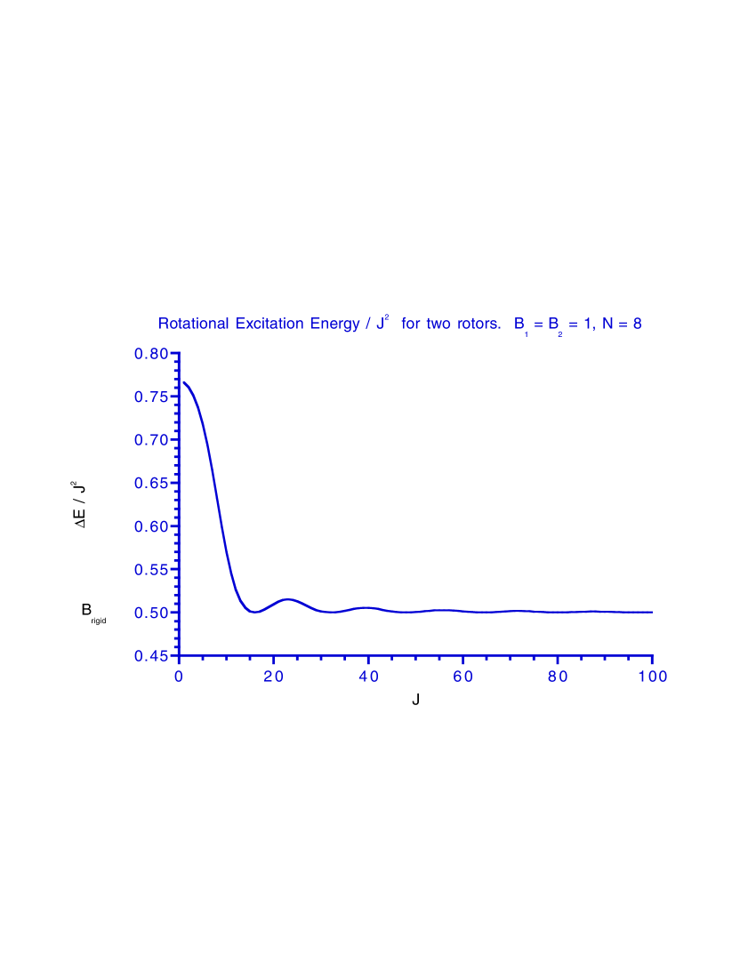
FIG. 5.: The rotational excitation energy, $\Delta E$, divided by $J^{2}$ as a function of the total rotational angular momentum quantum number, $J$. Calculated with $B_{1}=B_{2}=1$ and $V=100$. With rigid following of the helium, the plotted quantity should equal $B_{\rm rigid}$, which is indicated in the figure.

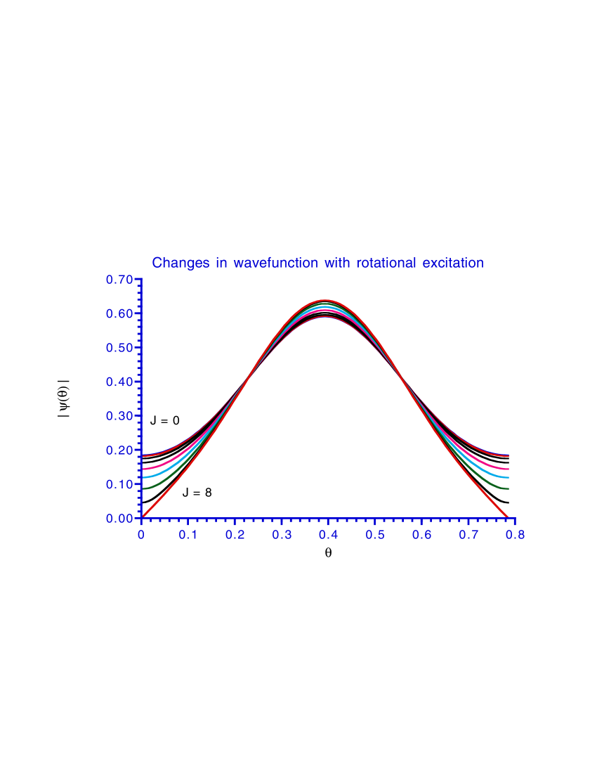
FIG. 6.: The absolute value of the vibrational wavefunction as a function of the relative orientation between molecule and 8 helium rotor. This quantity is plotted for angular momentum $J=0,1\ldots 8$.

REFERENCES

- [1] J. P. Toennies and A. F. Vilesov, Annual Reviews of Physical Chemistry 49, 1 (1998).
- [2] S. Grebenev et al., Physica B 280, 65 (2000).
- [3] K. K. Lehmann and G. Scoles, Science 279, 2065 (1998).
- [4] M. Hartmann, R. E. Miller, J. P. Toennies, and A. F. Vilesov, Science 272, 1631 (1996).
- [5] M. Hartmann, R. E. Miller, J. P. Toennies, and A. F. Vilesov, Physical Review Letters 95, 1566 (1995).
- [6] C. Callegari et al. (unpublished).
- [7] S. Grebenev et al., Journal of Chemical Physics 112, 4485 (2000).
- [8] S. Grebenev, J. P. Toennies, and A. F. Vilesov, Science 279, 2083 (1998).
- [9] Y. Kwon and K. B. Whaley, Physical Review Letters 83, 4108 (1999).
- [10] C. Callegari et al., Physical Review Letters 83, 5058 (1999).
- [11] E. B. Gordon and A. F. Shestakov, The Cluster Approach to Description of Atoms and Molecules Isolated by Helium, paper presented at the IV. Workshop on quantum Fluid Clusters, Ringberg Schloss, June, 2000.
- [12] E. Lee, D. Farrelly, and K. B. Whaley, Physical Review Letters 83, 3812 (1999).
- [13] A. Conjusteau et al., Journal of Chemical Physics 113, (2000), to be published.
- [14] J. M. Hutson, in Advances in Molecular Vibrations and Collision Dynamics, edited by J. M. Bowman and M. A. Ratner (JAI Press Inc., Greenwich, Connecticut, 1991), Vol. 1A, pp. 1–45.
- [15] A. J. Leggett, Physica Fennica 8, 125 (1973).
- [16] C. Callegari et al., Physical Review Letters 43, 1848 (2000).
- [17] C. Callegari et al. (unpublished).
- [18] P. J. Reynolds, D. M. Ceperley, B. J. Alder, and J. William A. Lester, Journal of Chemical Physics 77, 5593 (1982).
- [19] It was found that when Walkers moved very close to a node, they became trapped, due to the large size of the attempted steps introduced by the drift term combined with the ‘detailed balance’ correction selection criteria. When they also had large negative values of the local energy, these trapped walkers then grew in weight, leading to unphysical large negative values for the DMC estimate for the energy. This problem, which is part of the finite time step bias, was eliminated by killing walkers that failed the detail balance selection instead of keeping them at their previous location.