Four-wave mixing at maximum coherence and eliminated Doppler broadening controlled with the driving fields

Abstract.

New feasibity of coherent quantum control of four-wave mixing processes in a resonant Doppler-broadened medium are studied. We propose a technique which enables one to enhance the quantum efficiency of nonlinear optical conversion. At the same time, it allows one to decrease the required intensities of the fundamental beams compared to those necessary in the approach based on coherent population trapping. The major outcomes of the analysis are illustrated with numerical simulation addressed within a practical medium.

1 Introduction

The concept of quantum coherence and interference plays an important role in resonant nonlinear optics and spectroscopy [1]. Coherent coupling of laser radiation with multilevel quantum schemes has been used to manipulate energy level populations, nonlinear-optical response, refraction and absorption of a resonance medium [2]. Much attention has been shown to four-wave mixing (FWM) processes with maximal coherence on a Raman transition [3] based on the effect of coherence population trapping (CPT) [4], which allows a dramatic increase of conversion efficiency. In far-from-degenerate schemes, substantial Doppler broadening of the resonant quantum transitions gives rise to inhomogeneous coupling of the driving fields with the atoms in different velocity intervals. Therefore, under relatively low intensities, only a small fraction of the atoms can be concurrently coupled with both the fields driving the Raman transition and, as a consequence, the CPT conditions can not be fulfilled for the entire thermal velocity interval. This fundamental limitation in resonant nonlinear optics of gases substantially reduces the efficiency of the corresponding processes. The common methods of Doppler-free (DF) nonlinear spectroscopy entail ladder energy level schemes and equal frequency counter-propagating beams. This usually leads to large detunings from the intermediate resonance and consequently a decrease of the nonlinear susceptibility. Besides that, the method can not be applied to FWM processes in ladder schemes, due to the phase-matching requirements, and in Raman-type schemes due to the difference in frequencies of the coupled fields.

The technique, allowing one to overcome this obstacle by compensating for Doppler frequency shifts with light-induced ac-Stark shifts and thus enabling one to couple a wide velocity interval concurrently, has been proposed in [5]. This was developed in further publications [6] and most recently in publications [7] addressing FWM under conditions where CPT is not possible. Related effects in the absorption index were also investigated recently [8].

We further mean CPT as the process where two driving fields form nearly equal velocity-averaged populations of the levels at Raman transitions, while the velocity-averaged population of the intermediate state is much less. Along with this absorption and amplification indices for the couple fields reach minimum. On the other hand coherence in the Raman transition, which is origin of FWM, approaches maximum. That allows one to accomplish a maximum of the conversion efficiency. The conditions to achieve CPT may differ from those required for the DF Raman-type resonance. This present paper is aimed at investigating what are the most favorable conditions to accomplish effective FWM frequency conversion of radiation at a low fundamental radiation level. This also addresses the problem “nonlinear optics at the level a few photons per atom” [9].

2 Theoretical

2.1 Atomic coherence and energy level populations

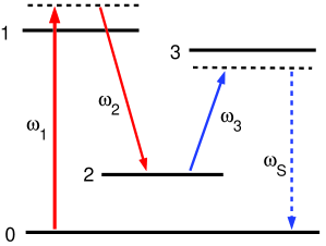
Fig. 1.: Energy level configuration

Consider a Raman-type scheme of FWM, $\omega_{S}=\omega_{1}-\omega_{2}+\omega_{3}$, depicted in Fig. 1, where $E_{1}$ and $E_{2}$ with frequencies $\omega_{1}$ and $\omega_{2}$ are traveling waves of the driving fields. The field $E_{3}$ with the frequency $\omega_{3}$ and generated radiation $E_{S}$ with the frequency $\omega_{S}$ are assumed weak (i.e., not changing the level populations). All waves are co-propagated. Initially, only the lower level $\it 0$ is populated. The steady-state solution for the off-diagonal elements of the density matrix (atomic coherence) can be found in the same form of traveling waves as the the resonant driving radiations. Then the equations for the density matrix amplitudes to the lowest order in $E_{3,S}$ can be written as

$$P_{01}r_{01}=-i\left[G_{01}(r_{1}-r_{0})-G_{21}r_{02}\right],\,P_{21}r_{21}=-i\left[G_{21}(r_{1}-r_{2})-G_{01}r_{20}\right],$$

$$P_{02}r_{02}=-i\left[G_{01}r_{12}-G_{12}r_{01}\right];$$ (1)

$$\mathchar 256\relax_{1}r_{1}=2\hbox{Re\,}[iG_{12}r_{21}+iG_{10}r_{01}],\,\mathchar 256\relax_{2}r_{2}=-2\hbox{Re\,}[iG_{12}r_{21}]+\gamma_{2}r_{1},$$

$$r_{0}+r_{1}+r_{2}=1;$$ (2)

$$P_{23}r_{23}=-i\left[-G_{23}r_{2}+G_{21}r_{13}-G_{03}r_{20}\right],$$

$$P_{03}r_{03}=-i\left[-G_{03}r_{0}+G_{01}r_{13}-G_{23}r_{02}\right],$$

$$P_{13}r_{13}=-i\left[G_{12}r_{23}-G_{23}r_{12}+G_{10}r_{03}-G_{03}r_{10}\right]\,$$ (3)

Here $r_{ij}$ and $r_{i}$ are the amplitudes of the off-diagonal and diagonal elements of the density matrix, $\displaystyle P_{ij}=\mathchar 256\relax_{ij}+i(\mathchar 266\relax_{l}-k_{l}v)$, $\displaystyle\mathchar 266\relax_{l}$ is the resonance detuning for the corresponding resonant field (e.g., $\displaystyle\mathchar 266\relax_{1}=\omega_{1}-\omega_{01}$), $\displaystyle\mathchar 256\relax_{ij}$ are homogeneous half-widths of the transitions (coherence relaxation rates), $v$ is the projection of the atom velocity on the direction of the wave vectors ${\bf k}_{l}$, $\displaystyle\gamma_{1,2}$ are relaxation rates from level $\it 1$ to $\it 0$ and from $\it 1$ to $\it 2$, accordingly, $\displaystyle\mathchar 256\relax_{1},\mathchar 256\relax_{2}$ are relaxation rates of the populations of the levels $\it 1$ and $\it 2$ accordingly, $\displaystyle G_{ij}=-{E_{j}d_{ij}}/{2\hbar}$ are the Rabi frequencies, and $d_{ij}$ are the electric dipole momenta of the transitions. Only the resonant couplings are accounted for.

The solution for the coherence $r_{02}$ and for those at the allowed transitions, which determine absorption and refraction at the frequencies $\omega_{1}$, $\omega_{2}$, $\omega_{3}$, are found in the form

$$r_{02}=\frac{G_{01}G_{12}}{\tilde{P}_{02}}\left\{\frac{\mathchar 257\relax r_{10}}{P_{01}}-\frac{\mathchar 257\relax r_{21}}{P_{21}^{*}}\right\}=\frac{G_{01}G_{12}}{P_{01}P_{21}^{*}}R_{02},$$

$$r_{01}=-i\frac{G_{01}}{P_{01}}\left\{\mathchar 257\relax r_{10}-\frac{|G_{12}|^{2}}{\tilde{P}_{02}}\left(\frac{\mathchar 257\relax r_{10}}{P_{01}}-\frac{\mathchar 257\relax r_{21}}{P_{21}^{*}}\right)\right\}=-i\frac{G_{01}}{P_{01}}R_{1},$$

$$r_{12}=-i\frac{G_{12}}{P_{21}^{*}}\left\{\mathchar 257\relax r_{21}+\frac{|G_{01}|^{2}}{\tilde{P}_{02}}\left(\frac{\mathchar 257\relax r_{10}}{P_{01}}-\frac{\mathchar 257\relax r_{21}}{P_{21}^{*}}\right)\right\}=-i\frac{G_{12}}{P_{21}^{*}}R_{2},$$

$$r_{23}=i\frac{G_{23}}{P_{23}}\left\{r_{2}\left(1-\frac{|G_{12}|^{2}}{P_{23}\tilde{P}_{13}}\right)-\frac{|G_{01}G_{12}|^{2}}{P_{03}\tilde{P}_{13}}\frac{R_{02}}{P_{01}P_{21}^{*}}-\frac{|G_{12}|^{2}}{P_{21}^{*}\tilde{P}_{13}}R_{2}\right\},$$

where $\mathchar 257\relax r_{ij}$ are intensity-dependent population differences, and $\tilde{P}_{02}$ and $\tilde{P}_{13}$ are two-photon denominators “dressed” by the driving fields:

$$\tilde{P}_{02}=P_{02}+\frac{|G_{01}|^{2}}{P_{21}^{*}}+\frac{|G_{12}|^{2}}{P_{01}},\quad\tilde{P}_{13}=P_{13}+\frac{|G_{01}|^{2}}{P_{03}}+\frac{|G_{12}|^{2}}{P_{23}}.$$ (4)

The coherence $r_{03}$ consists of two terms. One, $\bar{r}_{03}$, determines absorption and refraction at the frequency $\omega_{S}$, and the other, $\tilde{r}_{03}$, determines FWM at $\omega_{1}-\omega_{2}+\omega_{3}=\omega_{S}$:

$$\bar{r}_{03}=i\frac{G_{03}}{P_{03}}\left\{r_{0}\left(1-\frac{|G_{01}|^{2}}{P_{03}\tilde{P}_{13}}\right)-\frac{|G_{01}G_{12}|^{2}}{P_{23}\tilde{P}_{13}}\frac{R_{02}^{*}}{P_{01}^{*}P_{21}}+\frac{|G_{01}|^{2}}{P_{01}^{*}\tilde{P}_{13}}R_{1}^{*}\right\},$$ (5)

$$\tilde{r}_{03}=-i\frac{G_{01}G_{12}G_{23}}{P_{01}P_{21}^{*}P_{03}}\left\{R_{02}\left(\frac{|G_{01}|^{2}}{P_{03}\tilde{P}_{13}}-1\right)+\frac{P_{01}P_{21}^{*}}{\tilde{P}_{13}}\left(\frac{r_{2}}{P_{23}}+\frac{R_{2}}{P_{21}^{*}}\right)\right\},$$ (6)

where $\displaystyle P_{03}=\mathchar 256\relax_{03}+i(\mathchar 266\relax_{1}-\mathchar 266\relax_{2}+\mathchar 266\relax_{3}-k_{S}v)$ and $\quad k_{S}=k_{1}-k_{2}+k_{3}.$

Making use of the above equations, the solution for the populations can be found from (2) as

$$r_{2}=\frac{Y_{1}W_{02}-Y_{3}W_{01}}{Y_{1}Y_{4}-Y_{3}Y_{2}},\quad r_{1}=\frac{Y_{4}W_{01}-Y_{2}W_{02}}{Y_{1}Y_{4}-Y_{3}Y_{2}},\quad r_{0}=1-r_{1}-r_{2},$$ (7)

where

$$Y_{1}=2W_{01}-W_{02}+\gamma_{1},\quad Y_{2}=W_{02}+W_{01}+\mathchar 256\relax_{2},$$

$$Y_{3}=W_{02}-W_{21}-\gamma_{2},\quad Y_{4}=W_{02}+W_{21}+\mathchar 256\relax_{2},$$

and

$$W_{01}=2|G_{01}|^{2}\hbox{Re\,}\left\{\left(1-\displaystyle\frac{|G_{12}|^{2}}{P_{01}\tilde{P}_{02}}\right)/P_{01}\right\},$$

$$W_{21}=2|G_{12}|^{2}\hbox{Re\,}\left\{\left(1-\displaystyle\frac{|G_{01}|^{2}}{P_{21}^{*}\tilde{P}_{02}}\right)/P_{21}^{*}\right\},$$

$$W_{02}=2|G_{01}|^{2}|G_{12}|^{2}\hbox{Re\,}\left\{{1}/{P_{01}P_{21}^{*}\tilde{P}_{02}}\right\}.$$

2.2 Coherence-induced Doppler-free resonance

The appearance of a DF resonance and therefore the coupling of molecules from a wide velocity interval can be understood as follows. Ac-Stark shifts $\hbox{Im\,}\left\{{|G_{01}|^{2}}/{P_{21}^{*}}\right\}$ and $\hbox{Im\,}\left\{{|G_{12}|^{2}}/{P_{01}}\right\}$ in (4), originating from the coherence $r_{02}$, depend on the radiation intensity and frequency detunings. The later ones, in turn, depend on Doppler shifts. This allows one, by making judicious choice of the intensities and detunings of the driving fields, to “draw” into the dressed two-photon resonance all the molecules, independent of their velocities. In the limiting case, when the detuning from the intermediate resonance is much greater than the Doppler HWHM of the allowed optical transitions, the modified two-photon resonance described by the denominator $\tilde{P}_{02}$ can be presented in the lowest order in $k_{1,2}v/\mathchar 266\relax_{1,2}$ as

$$\tilde{P}_{02}=\tilde{\mathchar 256\relax}_{02}+i\tilde{\mathchar 266\relax}_{02}-i\left\{\left(1+\frac{|G_{12}|^{2}}{\mathchar 266\relax_{1}^{2}}\right)k_{1}-\left(1+\frac{|G_{01}|^{2}}{\mathchar 266\relax_{2}^{2}}\right)k_{2}\right\}v,$$ (8)

where $\displaystyle{\tilde{\mathchar 256\relax}_{02}}=\mathchar 256\relax_{02}+\frac{|G_{01}|^{2}}{\mathchar 266\relax_{2}^{2}}\mathchar 256\relax_{12}+\frac{|G_{12}|^{2}}{\mathchar 266\relax_{1}^{2}}\mathchar 256\relax_{01},\quad\tilde{\mathchar 266\relax}_{02}=\mathchar 266\relax_{1}-\mathchar 266\relax_{2}+\frac{|G_{01}|^{2}}{\mathchar 266\relax_{2}}-\frac{|G_{12}|^{2}}{\mathchar 266\relax_{1}}$ are the power broadened HWHM and ac-Stark shifted two-photon resonance detuning. From (8) it follows that the requirements for the induced Doppler-free resonance to be achieved are $\displaystyle\tilde{\mathchar 266\relax}_{02}=0$  and  $\displaystyle\tilde{k_{1}}=\tilde{k_{2}}$, where
$\displaystyle\tilde{k_{1}}v=\left(1+\frac{|G_{12}|^{2}}{\mathchar 266\relax_{1}^{2}}\right)k_{1}v$ and $\displaystyle\tilde{k_{2}}v=\left(1+\frac{|G_{01}|^{2}}{\mathchar 266\relax_{2}^{2}}\right)k_{2}v$
are intensity-dependent Doppler shifts. Eventually the equations take form

$$k_{1}\left(1+\displaystyle\frac{|G_{12}|^{2}}{\mathchar 266\relax_{1}^{2}}\right)-k_{2}\left(1+\displaystyle\frac{|G_{01}|^{2}}{\mathchar 266\relax_{2}^{2}}\right)=0,$$ (9)

$$\mathchar 266\relax_{1}\left(1-\displaystyle\frac{|G_{12}|^{2}}{\mathchar 266\relax_{1}^{2}}\right)-\mathchar 266\relax_{2}\left(1-\displaystyle\frac{|G_{01}|^{2}}{\mathchar 266\relax_{2}^{2}}\right)=0.$$ (10)

From (9)-(10) follows a cubic equation as $\mathchar 266\relax_{2}$:

$$\mathchar 266\relax_{2r}^{3}-(2-K)\mathchar 266\relax_{2r}^{2}\mathchar 266\relax_{1}-\mathchar 266\relax_{2r}|G_{01}|^{2}+K\mathchar 266\relax_{1}|G_{01}|^{2}=0,\quad K=k_{2}/k_{1},$$ (11)

which determines the detuning of field $E_{2}$, corresponding to the induced resonance, under given values of the Rabi frequency and detuning of field $E_{1}$. Here, the Rabi frequency of $E_{2}$ must be

$$|G_{12}|^{2}=\mathchar 266\relax_{1}^{2}\left\{K\left(1+\frac{|G_{01}|^{2}}{\mathchar 266\relax_{2r}^{2}}\right)-1\right\}.$$ (12)

One of the roots of the equation (11) corresponds to the dressed DF two-photon resonance,

$$\mathchar 266\relax_{2r}=(A^{1/3}+9B+2\mathchar 266\relax_{1}-\mathchar 266\relax_{1}K)/3,$$ (13)

where $\displaystyle A=9\mathchar 266\relax_{1}|G_{01}|^{2}(1-2K)+\mathchar 266\relax_{1}^{3}(8-12K+6K^{2}-K^{3})+3[3\mathchar 266\relax_{1}^{2}|G_{01}|^{4}\times$

$\displaystyle\times(-1-8K+11K^{2})+3\mathchar 266\relax_{1}^{4}|G_{01}|^{2}(-8K+12K^{2}-6K^{3}+K^{4})-3|G_{01}|^{6}]^{1/2}$,

$\displaystyle B=(|G_{01}|^{2}+4\mathchar 266\relax_{1}^{2}-4\mathchar 266\relax_{1}^{2}K+\mathchar 266\relax_{1}^{2}K^{2})/3A^{1/3},\quad K={k_{2}}/{k_{1}}.$

The conditions for the CPT and DF resonances may fit each other or differ, depending on the specific case. This and corresponding outcomes regarding FWM will be investigated below numerically for the most optimum situations, where the analytical solution can not be obtained.

3 Numerical analysis

The graphs presented below are computed numerically based on averages over the velocity equations (5), (6) and (7). For the numerical analysis we have used the parameters of the sodium dimer transition with the following wavelengths [10]: $X^{1}\mathchar 262\relax_{g}^{+}(v^{\prime\prime}=3,J^{\prime\prime}=43)$ – $B^{1}\mathchar 261\relax_{u}(6,43)(\lambda_{01}=488$ nm) – $X^{1}\mathchar 262\relax_{g}^{+}(13,43)$ $(\lambda_{21}=525$ nm) – $A^{1}\mathchar 262\relax^{+}_{u}(24,44)(\lambda_{23}=655$ nm) – $X^{1}\mathchar 262\relax_{g}^{+}(3,43)(\lambda_{13}=598$ nm). The corresponding homogeneous half-widths of the transition are 20.69, 23.08, 18.30 and 15.92 MHz, whereas the Doppler half-widths $\mathchar 257\relax\omega_{iD}$ are equal to 0.92, 0.85, 0.68 and 0.75 GHz. The numerical simulations allow us to analyze the velocity-averaged equation for the detunings, where the approximation taken in (8) is not valid.

3.1 Nonlinear resonances in FWM polarizations, in absorption indices and in the level populations

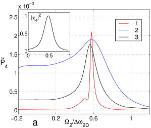
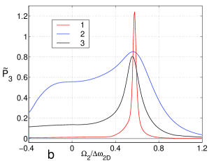
Fig. 2.: Normalized squared module of the FWM polarizations $\tilde{P}_{4}$ (a) and $\tilde{P}_{3}$ (b) vs the detuning of driving field $E_{2}$. The plots correspond to: 1– DF resonance, 2 – CPT, 3 – intermediate case, subplot – same resonance, but under weak fields.

Figure  2, plots 1 illustrate the coherence-induced compensation of Doppler shifts with ac-Stark shifts resulting in the resonance narrowing in the squared module of the velocity-averaged reduced nonlinear FWM polarizations

$|\tilde{P}_{4}|^{2}=(|\tilde{\chi}_{4}|^{2}/|\tilde{\chi}_{40}|^{2})|g_{01}|^{2}|g_{12}|^{2}$ [Fig.2 (a)] and $\displaystyle|\tilde{P}_{3}|^{2}=(|\tilde{\chi}_{3}|^{2}/|\tilde{\chi}_{40}|^{2})|g_{01}|^{2}|g_{12}|^{2}$ [Fig.2 (b)]. The nonlinear susceptibility is reduced by its maximum value in the same frequency range, but for negligibly-weak $E_{1}$ and $E_{2}$ fields, $\displaystyle{g_{01}}=G_{01}/\mathchar 257\relax\omega_{1D}$, $\displaystyle{g_{12}}=G_{12}/\mathchar 257\relax\omega_{2D}$. A substantial narrowing is seen from comparison with the subplot, presenting the spectral dependence of the velocity-averaged squared module of the same susceptibility, but in the negligibly weak fields, normalized to unity. The HWHM of the resonance in the subplot is approximately 70 MHz, which corresponds to the Doppler width of the nonperturbated Raman transition, whereas the HWHM of the resonance in plots 1 is 15 MHz. This indicates some power and residual Doppler broadening. The Rabi frequencies of the fields $E_{1}$ and $E_{2}$ are equal to 157 MHz and 85 MHz. The detuning of $E_{1}$ is equal to 413.8 MHz ($0.45\cdot\mathchar 257\relax\omega_{1D}$), and detuning of $E_{3}$ is equal to -695.5 MHz ($-1.02\cdot\mathchar 257\relax\omega_{3D}$). Plots 2 display the same dependences, but related to the CPT conditions (the half-width of this resonance in $|\tilde{P}_{4}|^{2}$ is 200 MHz). In this case, the required Rabi frequencies of $E_{1}$ and $E_{2}$ are equal to 351 MHz and 332 MHz, respectively, while the detunings are identical to those in plots 1. Plots 3 display the same dependence, but under the intensities, that provide narrowing in the intermediate range (HWHM of resonance is 70 MHz). In this case, the Rabi frequencies of the fields $E_{1}$ and $E_{2}$ are equal to 222 MHz and 235 MHz, respectively, whereas the detunings are the same as in the previous plots. The important outcome is that in the Doppler-free regime, larger FWM polarizations can be accomplished under lower driving fields. Also, we want to stress the substantial difference in magnitudes of the nonlinear susceptibilities $\chi_{4}$ and $\chi_{3}$, which follows from the interference of contributions of molecules in different velocity intervals to the macroscopic nonlinear polarizations.

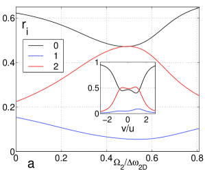
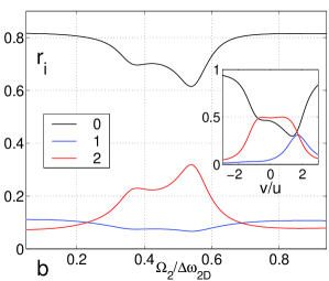
Fig. 3.: Velocity integrated population of the energy levels vs detuning of driving field $E_{2}$. a– near CPT and CPT regime, subplot – velocity distribution of the coherently trapped populations; b– near DF regime, subplot – velocity distribution of populations under DF regime.

Figure 3(a) shows dependence of the velocity integrated populations on the detuning of the field $E_{2}$, while the Rabi frequencies of $E_{1}$ and $E_{2}$ are equal to 351 MHz and 332 MHz, respectively so that the CPT conditions can be fulfilled under appropriate detuning. The subplot displays the distribution of the populations over velocities, whereas the detuning corresponds to the CPT regime for the velocity-integrated populations. Here $u$ is the thermal velocity with Maxwell envelope removed. The subplot indicates CPT for molecules in $v=0$; however, even inversion of the populations occurs in a relatively wide velocity intervals.

Figure 3(b) is computed for the Rabi frequencies of the fields $E_{1}$ and $E_{2}$ equal to 157 MHz and 85 MHz, respectively. The inset displays the distribution of the populations over velocities at the detuning corresponding to DF. The distribution is even more complicated compared to that in the previous case.

Figure 4 displays velocity-averaged absorption indices vs detuning of the field $E_{2}$.

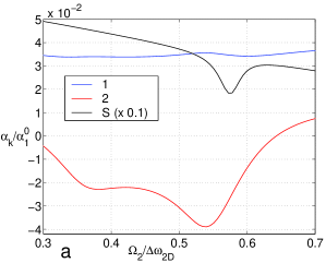
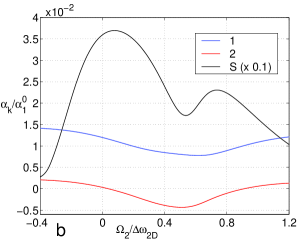
Fig. 4.: Velocity averaged absorption indices $\alpha_{1,2,S}$ near DF (a) and CPT (b) regimes vs detuning of the driving field $E_{2}$.

The intensities of the fields are the same as in the corresponding graphs given above. The graph 4 (a) shows a substantially decreased absorption index for the first field due to saturation effects, which is almost independent of the detuning of the second field because of its relative weakness. The second field experiences Stokes gain. The plot for the generated beam (reduced by 10) displays a nonlinear resonance in the absorption index. With growth of the second field intensity, so that CPT becomes possible, both absorption of the first and gain of the second driving field experience substantial decrease in the CPT regime. Absorption of the generated field dramatically changes as well (Figure 4 (a)).

A linear approximation in $k_{1,2}v/\mathchar 266\relax_{1,2}$ (see equation (8)) is valid for large detunings from the intermediate resonance. While for tuning close to the resonance, the concurrently coupled velocity interval decreases, the nonlinear response of the molecules grows. At the same time, absorption of the coupled radiations increases as well.

The output FWM generated radiation is determined by the interplay of the above considered processes. Moreover, resonant FWM may not be viewed as a sequence of the independent elementary acts of absorption, gain and FWM. Interference of these elementary processes plays a crucial role, even for a qualitative prediction of the spatial dynamics of the generated field [11]. Therefore, appropriate optimization is required in order to achieve the maximum FWM-generation output. In the next section, relevant results are presented based on the above analyzed dependencies.

3.2 Coherent quantum control of FWM in a double-$\mathchar 259\relax$ Doppler broadened medium

The solution of the Maxwell equations for the coupled traveling waves can be found in the form

$$E^{j}(z,t)=\hbox{Re\,}\{E_{j}(z)\exp[{\rm i}(\omega_{j}t-k_{j}z)]\},$$ (14)

where $k_{j}$ are complex wave number at the corresponding frequencies, $k_{j}=k_{j}^{\prime}-{\rm i}\alpha_{j}/2$. The set of the equations for the amplitudes, relevant to the case under consideration, is

$$\frac{d\,E_{1}}{dz}=-\frac{\alpha_{1}}{2}E_{1},\quad\frac{d\,E_{2}}{dz}=-\frac{\alpha_{2}}{2}E_{2},$$ (15)

$$\frac{d\,E_{3}}{dz}=-\frac{\alpha_{3}}{2}E_{3}+\sigma_{3}E_{1}^{*}E_{2}E_{S}\exp\{-i\mathchar 257\relax kz\},$$ (16)

$$\frac{d\,E_{S}}{dz}=-\frac{\alpha_{S}}{2}E_{S}+\sigma_{S}E_{1}E_{2}^{*}E_{3}\exp\{i\mathchar 257\relax kz\},$$ (17)

where $\sigma_{3}=i2\pi k_{3}\tilde{\chi_{3}}$ and $\sigma_{S}=i2\pi k_{S}\tilde{\chi_{S}}$ are cross coupling parameters, $\tilde{\chi_{3}}$ and $\tilde{\chi_{S}}$ are intensity-dependent nonlinear susceptibilities for the FWM processes $\omega_{S}\leftrightarrow\omega_{1}-\omega_{2}+\omega_{3}$ and $\mathchar 257\relax k=k_{S}-k_{1}+k_{2}-k_{3}$. The boundary conditions are $E_{l}(z=0)=E_{0l}$ ($l=1,2,3$) and $E_{S}(z=0)=0$. We assume that intensities of the weak waves with frequencies $\omega_{3}$ and $\omega_{S}$ are weak enough so that the change of the strong fields $E_{1,2}$ due to FWM conversion can be neglected. The quantum efficiency of conversion QEC of the radiation $E_{3}$ in $E_{S}$ is defined by the equation

$$\eta_{{\rm q}}=(\omega_{3}/\omega_{S})|E_{S}(z)/E_{3}(0)|^{2}\exp(-\alpha_{S}z).$$ (18)

Assuming that the condition of phase matching $\mathchar 257\relax k^{\prime}=0$ can be ensured (e.g., with a buffer gas), the solution for QEC of the above given equations can be expressed as

$$\eta_{q}=\displaystyle\frac{\omega_{3}}{\omega_{S}}\bigl{|}\displaystyle\frac{\sigma_{S}}{g_{0}}\bigl{|}^{2}\bigl{|}E_{01}E_{02}\bigl{|}^{2}\exp\left[(\hbox{Re\,}g_{0}-\frac{\alpha}{2})z\right]\bigl{|}1-\exp(-g_{0}z)\bigr{|}^{2},$$

$$g_{0}=\left[\left[(\alpha_{1}+\alpha_{2}+\alpha_{3}-\alpha_{S}/2)\right]^{2}+4\sigma_{S}\sigma_{3}\bigl{|}E_{01}E_{02}\bigl{|}^{2}\right]^{1/2},\quad\alpha=\alpha_{3}+\alpha_{S}.$$

These formulas account for nonlinear resonances both in FWM nonlinear polarizations and in absorption indices. In order to compute the absolute magnitude of QEC (under the assumption of $\mathchar 257\relax k^{\prime}=0$) we have used the data for the Frank-Condon factors of 0.068, 0.142, 0.02 and 0.036 for the transition with wavelengths $\lambda_{01}$, $\lambda_{21}$, $\lambda_{23}$ and $\lambda_{03}$ accordingly.

Figure 5 presents a numerical simulation of the evolution of QEC along the vapor cell. The distance is scaled to the resonance optical density $\alpha_{01}z$ with the driving fields being turned off. The plot 1 corresponds to the case where the conditions for Doppler compensation at the transition 0–2 are fulfilled on the entrance of the cell. The Doppler-free resonance would be narrower if one of the coupled fields were weak. However, that would give rise to larger absorption and to decreased nonlinear FWM polarization. The optimization accounting for the change of the driving fields along the medium also shows that it does not substantially change the optimum input intensity values for the plots presented in Fig. 5. Plot 2 displays the same dependence, but for the optimum CPT conditions. Alternatively, they are not optimum for the elimination of Doppler broadening.

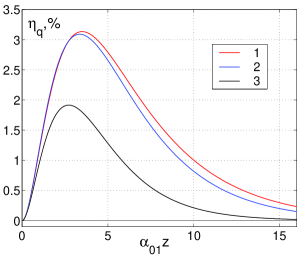
Fig. 5.: QEC vs optical density of the medium. 1 – DF, 2 – CPT, 3 – intermediate regimes.

The maxima of these two curves are comparable, but in the Doppler- free regime, quite lower intensities of the fundamental radiations are required. Plot 3 displays a similar dependence in the intermediate case. All intensities and detunings are identical to those used for computing the previous figures.

For the transitions under consideration, the Rabi frequency on the level of 100 MHz corresponds to powers of about 100 mW focused on a spot on the order of $10^{-4}$ cm², which can be realized with common cw lasers with the confocal parameter of focusing of about 2.5 cm. At a temperature of about 700 K, the optimum optical density of the dimers is achievable for vapor lengths of about 2 cm. This is in accord with the parameters of typical cw FWM experiments (see, e.g. [10]).

The above indicated intensity corresponds to about $10^{11}$ photons per cubic centimeter. Accounting for the molecule number density at the indicated temperature, which is on the order on $10^{13}$ cm^-3, we have about $10^{-2}$ photon/molecule.

4 Conclusion

Coherent control of populations [12] and of four-wave mixing [13] with pulses shorter than the dephasing time $T_{2}$ has proven to be a powerful tool for manipulating nonlinear-optical and chemical properties of free atoms and molecules. In these cases, maximum coherence can be achieved as a result of Rabi oscillations of the two-photon transition, and the required driving intensity is much higher than that proposed in this paper. Consequently, Doppler broadening of the coupled transitions does not play an important role.

On the contrary, this paper considers coherent quantum control of resonant four-wave mixing processes, where Doppler-broadening of a double-$\mathchar 259\relax$ medium is the factor of crucial importance. An approach enabling one to enhance the efficiency of nonlinear optical conversion and, at the same time, to decrease the required intensity for the fundamental pump beams is proposed. This approach is based on the elimination of Doppler broadening of the resonant two-photon transition. The advantages of the proposed method as compared to those based on coherent population trapping, where inhomogeneous broadening may play important role too, are illustrated with numerical simulations for realistic experimental schemes. The results obtained contribute to the field of nonlinear optics at the level of several photons per atom, which is currently attracting growing interest.

5 Acknowledgments

TFG and AKP thank U.S. National Research Council - National Academy of Sciences for support of this research through the international Collaboration in Basic Science and Engineering (COBASE) program. AKP and ASB acknowledge funding support from the International Association of the European Community for the promotion of co-operation with scientists from the New Independent States of the former Soviet Union (INTAS) (grant INTAS-99-19) and Russian Foundations for Basic Research (grant 99-02-39003) and from the Center on Fundamental Natural Sciences at St. Petersburg University (grant 97-5.2-61).

References

-
1.
S.G. Rautian and A.M. Shalagin, Kinetic
Problems of Nonlinear Spectroscopy Amsterdam: Elsevier 1991
A.K. Popov, Introduction in Nonlinear Spectroscopy Novosibirsk: Nauka 1983 (in Russian) -
2.
For review see, e.g. Papers from Atomic Coherence and
interference, Crested Butte Workshop 1993: Journal of the European Optical Society B
6 (1994) No 4
A review of early Russian works can be found in: A.K. Popov and S.G. Rautian: Proc. SPIE 2798 (1996) 49 (review) Coherent Phenomena and Amplification without Inversion (A.V. Andreev, O. Kocharovskaya and P. Mandel, Editors), http://www.spie.org/web/abstracts/2700/2798.html, http://xxx.lanl.gov/abs/quant-ph/0005114
A.K. Popov: Bull. Russ. Acad. Sci., Physics 60 (1996) 927 (Allerton Press. Inc) [Transl. from: Izvestiya RAN, ser. Fiz. 60 (1996) 92] (review), http://xxx.lanl.gov/abs/quant-ph/0005108
A.K. Popov: Proc. SPIE 3485 (1998) 252 (S.G. Rautian, I.M. Beterov, N.M. Rubtsova, Editors), http://www.spie.org/web/abstracts/3400/3485.html, http://xxx.lanl.gov/abs/quant-ph/0005118 -
3.
Maanesh Jain, Hui Xia, G.Y. Yin, A.J. Merriam,
and S.E. Harris: Phys. Rev. Lett. 77 (1996) 4326,
http://ojps.aip.org/prlo/
Y. Li and M. Xiao: Opt. Lett. 21 (1996) 1064
B. Lu, W.H. Burkett, and M. Xiao: Opt. Lett. 23 (1998) 804, http://ojps.aip.org/olo/
A.V. Sokolov, G.Y. Yin, and S.E. Harris: Proc. SPIE 3485 (1998) 26 (S.G. Rautian, I.M. Beterov, N.M. Rubtsova, Editors)
V.G. Arkhipkin, S.A. Myslivets, D.V. Manushkin, and A.K. Popov: ibid, 525, http://www.spie.org/web/abstracts/3400/3485.html
V.G. Arkhipkin, S.A. Myslivets, D.V. Manushkin, and A.K. Popov: Quantum Electronics 28 (1998) 637, http://turpion.ioc.ac.ru/
A.J. Merriam, S.J. Sharpe, H. Xia, D. Manuszak, G.Y. Yin, and S.E. Harris: Opt. Lett. 24 (1999) 625, http://ojps.aip.org/olo/ -
4.
B.D. Agap’ev, M.B. Gorniy, B.G. Matisov,
Yu.V. Rojdestvenskiy: Usp. Fiz. Nauk 163 (1993) 1
E. Arimondo: Progress in Optics XXXV (1996) 257 -
5.
T.Ya. Popova, A.K. Popov, S.G. Rautian, A.A.
Feoktistov: Sov. Phys. JETP, 30, 243 (1970) [Translated from Zh. Eksp. Teor.
Fiz. 57, 444 (1969)], http://xxx.lanl.gov/abs/quant-ph/0005081
C. Cohen-Tannoudji: Metrologia 13 (1977) 161 -
6.
C. Cohen-Tannoudji, F. Hoffbeck, S. Reynaud:
Opt. Comm. 27 (1978) 71
A.K. Popov and L.N. Talashkevich: Optics Comm. 28(1979) 315
S. Reynaud, M. Himbert, J. Dupon-Roc, H.H. Stroke and C. Cohen-Tannoudji: Phys. Rev. Lett. 42 (1979) 756
A.K. Popov and V.M. Shalaev: Optics Comm. 35 (1980) 189
A.K. Popov and V.M. Shalaev: Opt. Spectrosc. 49(1981) 336 [Transl. from Opt.Spektrosk. 49(1980) 617]
A.K. Popov and V.M. Shalaev: Sov. J. Quant. Electr. 12 (1982) 289 [Transl. from Kvant. Electr. 9 (1982) 488]
S. Reynaud, M. Himbert, J. Dalibard, J. Dupont-Roc and C. Cohen-Tannoudji: Opt. Comm. 42 (1982) 39 -
7.
A.K. Popov and A.S. Bayev:
JETP Letters 69 (1999) 110,
http://ojps.aip.org/jetplo/
A.K. Popov and A.S. Bayev: Phys. Rev. A 62, 025801 (2000), http://ojps.aip.org/prao/ -
8.
G. Vemuri, G.S. Agarwal, B. Rao:
Phys. Rev. A 53 (1996) 2842
Yifu Zhu and T.N. Wasserlauf: Phys. Rev. A 54 (1996) 3653
Yifu Zhu, T.N. Wasserlauf and P. Sanchez: Phys. Rev. A 54 (1996) 4500
A.K. Popov and V.M. Shalaev: Phys. Rev. A 59 (1999) 946, http://ojps.aip.org/prao/ - 9. S.E. Harris and L.V. Hau: Phys. Rev. Lett. 82 (1999) 4611, http://ojps.aip.org/prlo/
- 10. S. Babin, U. Hinze, E. Tiemann and B. Wellegehausen: Opt. Lett. 21 (1996) 1186, http://ojps.aip.org/olo/
- 11. A.K. Popov, S.A. Myslivets, E. Tiemann, B. Wellegehausen and G. Tartakovsky: JETP Letters 69 (1999) 912, http://ojps.aip.org/jetplo/.
- 12. T.Rickes, L.P. Yatsenko, S.Steuerwald, T.Halfmann, B.W.Shore, N.V.Vitanov, and K.Bergmann: J.Chem.Phys. 113 (2000) 534 http://www.physik.uni-kl.de/w_bergma/Publications/1997-2000/
-
13.
O. Kittelmann, J. Ringling, A. Nazarkin, G. Korn, and I. V. Hertel:
Phys. Rev. Lett. 76 (1996) 2682,
http://ojps.aip.org/prlo/;
A. Nazarkin, G. Korn, O. Kittelmann, J. Ringling, and I. V. Hertel: Phys. Rev. A 56 (1997) 671 http://ojps.aip.org/prao/