Re-examination of the “3/4-law” of Metabolism

Abstract

We examine the scaling law $B\propto M^{\alpha}$ which connects organismal metabolic rate $B$ with organismal mass $M$, where $\alpha$ is commonly held to be $3/4$. Since simple dimensional analysis suggests $\alpha=2/3$, we consider this to be a null hypothesis testable by empirical studies. We re-analyze data sets for mammals and birds compiled by Heusner, Bennett and Harvey, Bartels, Hemmingsen, Brody, and Kleiber, and find little evidence for rejecting $\alpha=2/3$ in favor of $\alpha=3/4$. For mammals, we find a possible breakdown in scaling for larger masses reflected in a systematic increase in $\alpha$. We also review theoretical justifications of $\alpha=3/4$ based on dimensional analysis, nutrient-supply networks, and four-dimensional biology. We find that present theories for $\alpha=3/4$ require assumptions that render them unconvincing for rejecting the null hypothesis that $\alpha=2/3$.

I Introduction

The “$3/4$-law” of metabolism states that organismal basal metabolic rate, $B$, is related to organismal mass, $M$, via the power law (kleiber32, ; kleiber61, ; bonner83, ; calder84, ; schmidt-nielsen84, ; peters83, )

$$B=cM^{\alpha},$$ (1)

where $\alpha$ is believed to be $3/4$. The assumption that $\alpha=3/4$ is relevant in medicine (mordenti86, ; anderson97, ; mahmood99, ), nutrition (cunningham80, ; pike84, ; burger91, ), and ecology (damuth81, ; lindstedt86, ; calder84, ; carbone99, ), and has been the subject of a series of theoretical debates (blaxter65, ; heusner82b, ; feldman82, ; economos83, ; prothero84a, ; feldman95, ). It has been oft quoted that quarter-power scaling is ubiquitous in biology (calder84, ; west97, ). Such quarter-law scaling reinforces, and is reinforced by, the notion that basal metabolic rate scales like $B\propto M^{3/4}$.

Nevertheless, the reasons, biological or otherwise, for why $\alpha=3/4$ have remained elusive and their elucidation stands as an open theoretical problem. A recent surge of interest in the subject, including our own, has been inspired by the elegant attempt of West, Brown and Enquist (west97, ) to link nutrient-supply networks to metabolic scaling. This work suggests that a fundamental understanding of the relationship between basal metabolism and body size is within our grasp and that closer inspection of both theory and data are duly warranted.

In this paper we work from the null hypothesis that $\alpha=2/3$. In a resting state, heat is predominantly lost through the surface of a body. One then expects, from naive dimensional analysis, that basal metabolism scales as surface area which scales as $V^{2/3}$ where $V$, volume, is proportional to $M$ presuming density is constant. This scaling of surface area with mass has found strong empirical support in organismic biology (hemmingsen60, ; schmidt-nielsen84, ; calder84, ; heusner87, ). Such a surface law of metabolism was first expounded in the nineteenth century (rubner1883, ). Later observations of deviations from $\alpha=2/3$ eventually led to its replacement by $\alpha\simeq 0.72$–$0.73$ which was then supplanted by the simpler $\alpha=3/4$ (brody45, ; hemmingsen60, ; kleiber61, ). The widespread agreement that $\alpha=3/4$ is due largely to the formative influence of Kleiber (kleiber32, ; kleiber61, ; schmidt-nielsen84note, ) and has been accepted and used as a general rule for decades (blaxter65, ).

We re-examine empirical data available for metabolic rates of homoiotherms as well as carefully review both recent and historical theoretical justifications for $\alpha=3/4$. Our statistical analysis of data collated by Heusner (heusner91, ) for 391 species of mammals and by Bennett and Harvey (bennett87, ) for 398 species of birds shows that over considerable, but not all, ranges of body size, the hypothesis $\alpha=2/3$ is not rejected by the available data. We also review empirical studies by Bartels (bartels82, ), Hemmingsen (hemmingsen60, ), Brody (brody45, ), and Kleiber (kleiber32, ) and find the data, upon re-examination, to be supportive of our interpretations. We then examine theoretical attempts to connect metabolic rate to mass. These include approaches based on dimensional analysis (gunther82, ; economos82, ; gunther85, ; bonner83, ; heusner82a, ; feldman95, ), four-dimensional biology (blum77, ; west99, ), and nutrient-supply networks (west97, ; banavar99, ). We find that none of these theories convincingly show that $\alpha=3/4$, rather than $\alpha=2/3$, should be expected.

However, we do not suggest that the $3/4$-law should be replaced by a $2/3$-law of allometric scaling. We instead argue for a more general approach to the subject, using $\alpha=2/3$ as a null hypothesis which should be tested by empiricists when considering $\alpha\neq 2/3$, and acknowledge the possibility of deviations from simple scaling.

II Measuring the metabolic exponent

The history of metabolic scaling may be traced through a series of heavily cited empirical papers, some of which are composed of very few data points. In order to better understand the scaling of metabolic rate, we work back in time, calculating $\alpha$ and deviations from uniform scaling for data from Heusner (heusner91, ), Bennett and Harvey (bennett87, ), Bartels (bartels82, ), Hemmingsen (hemmingsen60, ), Brody (brody45, ), and Kleiber (kleiber32, ). These papers represent some of the most influential, widely cited, and often controversial papers in the field. Our re-analysis of the data demonstrates that $\alpha=2/3$ should not be rejected for mammals with mass less than approximately $10$–$35$ kg, and a similar analysis of metabolic data for birds demonstrates $\alpha=2/3$ should not be rejected for birds in general.

We have used the same methods to calculate $\alpha$ and its dependence on $M$ in all cases where data is available. Slopes and intercepts are determined using standard linear regression in log-space taking $M$ to be the independent variable. The standard correlation coefficient is denoted by $r$ while that obtained using the Spearman rank ordering (press92, ) is written as $r_{s}$. When data is not available we have attempted to classify the data sets in terms of the original calculations of $\alpha$ and its dependence on $M$.

II.1 Heusner (1991)

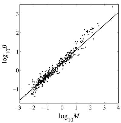
Figure 1: Metabolic rate, $B$ (watts), as a function of mass, $M$ (kg), for 391 species of mammals. Data taken from Heusner (heusner91, ). The straight line represents the best fit for the 357 species with mass less than 10 kg where the $\alpha=0.668\pm 0.019$. The upward deviations for species with larger mass (see Table 1) may indicate a real biological difference but may also be due to the paucity of data.

Data on basal metabolic rate for 391 mammalian species compiled by Heusner (heusner91, ) is reproduced in Figure 1. Heusner proposed that species could be separated into two groups, one of animals whose basal metabolism is normally distributed about a regression line and one of statistical outliers. Both groups were found by Heusner to satisfy a $2/3$-law for metabolism.

The results of simple regression analysis over various mass ranges for Heusner’s data are shown in Table 1. We observe a break in scaling occurring at around $M\simeq 10$ kg. For those ranges with an upper mass $M_{\mbox{\scriptsize{max}}}\leq 10$ kg, $\alpha=2/3$ appears to be robust. Note that the data comprises 179 species of the order rodentia ranging over more than three orders of magnitude of mass from 0.007 kg to 26.4 kg. On separating out these samples, we still find $\alpha=0.675\pm 0.025$ for the remaining species with $M\leq 10$ kg and $\alpha=0.681\pm 0.035$ for the rodentia species.

$M_{\mbox{\scriptsize{max}}}$	$N$	$\alpha$	$\sigma(\alpha)$	0.05	0.01
$0.01$	17	0.454	0.441	[-0.811,1.719]	[-1.294,2.202]
$0.032$	81	0.790	0.093	[0.545,1.034]	[0.473,1.106]
$0.1$	167	0.678	0.038	[0.578,0.778]	[0.550,0.806]
$1$	276	0.662	0.016	[0.620,0.704]	[0.608,0.716]
$10$	357	0.668	0.010	[0.643,0.693]	[0.636,0.700]
$32$	371	0.675	0.009	[0.651,0.698]	[0.645,0.705]
$100$	381	0.698	0.009	[0.675,0.720]	[0.668,0.727]
$1000$	390	0.707	0.008	[0.686,0.728]	[0.680,0.734]
$3670$	391	0.710	0.008	[0.689,0.731]	[0.684,0.737]

Table 1: The exponent $\alpha$ measured for varying ranges of mass, $M<M_{\mbox{\scriptsize{max}}}$ (kg), for Heusner’s data (heusner91, ). For each mass range, $N$ is the sample number and the errors, $\sigma(\alpha)$, are for two standard deviations. The 95% and 99% confidence intervals of $\alpha$ are listed in the last two columns. For small mammals ($M\leq 0.01$ kg, 17 species) a large error is apparent but for increasing $M_{\mbox{\scriptsize{max}}}$, $\alpha$ centers around $2/3$. A gradual upwards drift in $\alpha$ is evident for $M_{\mbox{\scriptsize{max}}}>10$ kg.

Upon addition of mammals with mass exceeding $10$ kg, the exponent steadily increases. Given the small number of samples of large mammals, one can only speculate on the reason for this possible deviation. Primarily, it may indicate a real upwards deviation from scaling, with larger organisms actually having greater metabolic rates than predicted by $\alpha=2/3$ (bartels82, ; economos83, ; heusner91a, ). Larger organisms are reported to scale allometrically in form so such a deviation may be a result of changes in body shape and hence surface area (bonner83, ; calder84, ). Support for this notion comes from Economos (economos82, ) who finds the relationship between mammalian head-and-body length and mass is better fit by two scaling laws rather than one. He identifies 20 kg as a breakpoint, which is in accord with our findings here, suggesting that geometric scaling holds below this mass while allometric quarter-power scaling holds above. The upper scaling observed by Economos could also be viewed as part of a gradual deviation from geometric scaling.

The upwards shift of metabolic rates for larger mammals could otherwise point to problems of measurement (note the corrections for elephants in Brody’s data (brody45, )), an evolutionary advantage related to larger brain sizes (jungers85, ; allman99, ), or the lack of competition for ecological niches for large mammals creating a distinction with smaller mammals.

II.2 Bennett and Harvey (1987)

Birds show strong support for not rejecting the null hypothesis $\alpha=2/3$. Figure 2 shows metabolic data for 398 distinct bird species taken from Bennett and Harvey (bennett87, ; bennett87note, ). We find here that $\alpha=0.666\pm 0.013$ in agreement with Bennett and Harvey’s calculations. Lasiewski and Dawson (lasiewski67, ) similarly found that $\alpha=0.668$ for a smaller set of data. Attempts to reconcile the $3/4$-law with these measurements have centered around the division of birds into passerine (perching birds) and non-passerine species (non-perching birds). Lasiewski and Dawson, for example, found exponents $0.724$ and $0.723$ for passerine and non-passerine species respectively. Though this is not an arbitrary division (core temperatures are thought to differ by 1–${2}^{\circ}\mbox{C}$), later work by Kendeigh (kendeigh77, ) finds exponents ranging from $0.668$–$0.735$ when passerines and non-passerines are grouped according to different measurement conditions (winter vs. summer, etc.).

Similar distinctions between intra- and inter-species scaling have been raised in the study of metabolic scaling for mammals where it has been suggested that $\alpha=2/3$ for single species comparisons and $\alpha=3/4$ holds across differing species (schmidt-nielsen84, ; heusner82b, ; bonner83, ). Bennett and Harvey (bennett87, ) also found that $\alpha$ depends on the level of taxonomic detail one is investigating. It remains unclear whether such subdivisions reflect relevant biological distinctions or underlying correlations in the choice of taxonomic levels.

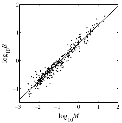
Figure 2: Metabolic rate, $B$ (watts), as a function of mass, $M$ (kg), for 398 species of birds taken from Bennett and Harvey (bennett87, ). The straight line is the result of a regression analysis which gives $\alpha=0.666\pm 0.014$.

II.3 Bartels (1982)

Bartels (bartels82, ) analyzes a set of approximately 85 mammalian species. Although data is not provided in the paper, a summary of his results can be found in Table 2. Bartels finds $\alpha=0.66$ (no error estimate is given) for mammals with mass between $2.4\times 10^{-3}$ kg and $3800$ kg and concludes that the deviation from the expected $3/4$ scaling is due to the variations in metabolic rates of small animals. This lends further weight to our conjecture that there may be a mass dependence of metabolic rate scaling.

$M_{\mbox{\scriptsize{min}}}$	$M_{\mbox{\scriptsize{max}}}$	$N$	$\alpha$	$r$
$2.4\times 10^{-3}$	3800	$\simeq 85$	0.66	0.99
$2.4\times 10^{-3}$	0.26	$\simeq 40$	0.42	0.76
0.26	3800	$\simeq 45$	0.76	0.99

Table 2: Exponents measured for varying ranges of mass (kg), $M_{\mbox{\scriptsize{min}}}\leq M\leq M_{\mbox{\scriptsize{max}}}$ according to Bartels (bartels82, ). Here $N$ is the sample number and $r$ is the correlation coefficient.

II.4 Hemmingsen (1960)

Hemmingsen’s data set (hemmingsen60, ) for mammals comprises 15 data points with masses between 0.01 kg and 3500 kg. Most of his data is derived from earlier work by Brody. He states that the data is well modeled by a power law with $\alpha=0.73$. To reach this conclusion he does not compute the power law of best fit, but rather, the “straight line…was chosen corresponding to [$\alpha=$]$0.73$, as established by Kleiber and also by Brody.”

Hemmingsen also finds that a $3/4$-law holds for unicellular organisms. Hemmingsen’s work has been cited extensively in support of the claim that the $3/4$-law is a universal biological phenomenon (peters83, ; schmidt-nielsen84, ; calder84, ; west97, ). A careful re-examination of Hemmingsen’s work by Prothero (prothero86b, ) showed that $\alpha$ can range from approximately 0.60 to 0.75 depending on which unicellular organisms are included in the regression. In addition to these questions about scaling for unicellular life, Patterson (patterson92b, ; patterson92a, ) has theoretically shown for aquatic inverterbrates and algae that the scaling exponent can range from 0.31 to 1.00 depending on the mass transfer mechanisms involved. We agree with Prothero’s conclusions that “a three-quarters power rule expressing energy metabolism as a function of size in unicellular organisms generally is not at all persuasive” (prothero86b, ).

II.5 Brody (1945)

One of the most influential works on scaling and metabolism is that of Brody (brody45, ). Indeed, the scaling law for metabolism is sometimes cited as the Brody-Kleiber law. Brody compiles a list of metabolic rates for 67 mammals. The complete data set yields $\alpha=0.73\pm 0.01$. However, on inspection, one makes the surprising observation that 32 data points are artificial in that most of these are calculated using previously determined empirical equations while a few have been corrected to account for variations in animal activity. Using the remaining set of 35 animals we nevertheless find $\alpha=0.72\pm 0.02$. It is also important to note that Brody’s research was done before the widespread use of electrocardiography and, as pointed out by Kinnear and Brown (kinnear67, ), Brody’s data may contain overestimations of basal metabolic rate.

We re-analyze Brody’s raw, uncorrected data for mammals over different mass ranges as shown in Table 3. Again, an increase in $\alpha$ is observed for ranges of larger masses. This is consistent with the results from Heusner’s and Bartel’s data which suggest a deviation from perfect scaling with increase in mass. Furthermore, it is evident that $\alpha=0.72$ as calculated by regression on the full data set is misleading. We reiterate that we are not suggesting that there is any robust scaling law for large masses. The results of the regression analysis merely suggest a dependence of $\alpha$ on the mass ranges being considered and that a strict power law may not be appropriate.

$M_{\mbox{\scriptsize{min}}}$	$M_{\mbox{\scriptsize{max}}}$	$N$	$\alpha$	$r_{s}$
0.016	1	19	$0.673\pm 0.061$	0.91
0.016	10	26	$0.709\pm 0.020$	0.96
10	922	9	$0.760\pm 0.085$	0.95
0.016	922	35	$0.718\pm 0.022$	0.98

Table 3: Results of regression on Brody’s data (brody45, ) over different mass intervals, $M_{\mbox{\scriptsize{min}}}<M<M_{\mbox{\scriptsize{max}}}$. An increase in $\alpha$ occurs for ranges over larger masses. Here, $N$ is the number of data points and $r_{s}$ is the Spearman correlation coefficient.

II.6 Kleiber (1932)

In his now-famous paper on metabolic rate, Kleiber analyzed 13 species of mammals with average mass ranging from 0.15 to 679 kg (kleiber32, ). We find the scaling exponent for the data to be $0.738\pm 0.016$. Again we consider the possibility of a crossover and separate the data into a set of 5 species with $M<10$ kg and 8 species with $M>10$ kg. For $M<10$ kg, $\alpha=0.667\pm 0.043$ while for $M>10$ kg, $\alpha=0.754\pm 0.048$. These results are again consistent with our assertion of a mass-dependent $\alpha$. Nevertheless, it is important to remain mindful of the relative paucity of data in these influential works.

III Fluctuations about scaling

The next logical step after measuring the metabolic exponent and systematic deviations thereof is to consider fluctuations about the mean. This is seldom done with power law measurements (dodds2000ua, ) and researchers concerned with the predictive power of a scaling law for metabolic rate have often pointed to organisms that deviate from predictions as being either problematic or different (brody45, ; bartels82, ; schmidt-nielsen84, ; heusner91, ). We take the view that fluctuations are to be expected and quantified appropriately.

We thus generalize the relation $B=cM^{\alpha}$ by considering $P(B\,|M)$, the conditional probability density of measuring a metabolic rate, $B$, given a mass, $M$,

$$P(B\,|M)=M^{-\alpha}f(B/M^{\alpha})$$ (2)

where the leading factor of $M^{-\alpha}$ is for normalization and $\int_{0}^{\infty}f(x)dx=1$.

Our null hypothesis is that fluctuations are Gaussian in logarithmic space, i.e., $f$ is a lognormal distribution. Gaussian fluctuations are typically assumed in statistical inferences made using regression analysis (degroot1975, ). Demonstrating that $f$ is not inconsistent with a normal distribution will therefore allow us to use certain hypothesis tests in the following section.

If equation (2) is correct then the sampled data can be rescaled accordingly to reconstruct $f$, the scaling function. To do so, one must first determine $\alpha$. We suggest the most appropriate estimate of $\alpha$ corresponds to the case when the residuals about the best fit power law are uncorrelated with regards to body mass. This is similar to techniques used in the analysis of partial residuals (hastie87, ) and we make use of it later. We obtain residuals for the range $0.5\leq\alpha\leq 1.5$ where the prefactor $c$ of $B=cM^{\alpha}$ is determined via least squares. The Spearman correlation coefficient $r_{s}$ is then determined for the residuals and recorded as a function of $\alpha$. We then take the value of $\alpha$ for which $r_{s}=0$ as the most likely underlying scaling exponent.

We find $r_{s}=0$ when $\alpha\simeq 0.665$ for mammals using Heusner’s data with $M\leq 10$ kg and $r_{s}\simeq-0.42$ when $\alpha=3/4$. For the entire range of masses in bird data of Bennett and Harvey, $r_{s}=0$ when $\alpha\simeq 0.671$.

With these results in hand, we extract $f$ for mammals and birds, the results for mammals being shown in Figure 3. We find the form of $f$ agrees qualitatively with a lognormal. In order to quantify the quality of this agreement we employ the Kolmogorov-Smirnov test (degroot1975, ), a non-parametric test which gives a significance probability ($p$-value) for whether or not a sample comes from a hypothesized distribution. Not having a hypothesis for the value of the standard deviation, we take two approaches to deal with this problem. Asserting the measured sample standard deviation $\sigma$ to be that of the underlying normal distribution, we calculate the corresponding significance probability, $p$. Alternatively, an estimate of $\sigma$, $\sigma^{\ast}$, may be obtained by finding the value of $\sigma$ which maximizes $p$ such that $p(\sigma^{\ast})=p^{\ast}$. Results for both calculations are found in Table 4. All $p$-values are above 0.01, i.e., none show very significant deviations. Additionally, the $p$-value for only the case of the birds using $\sigma$ estimated from the data falls below 0.05 indicating its departure is significant, but this is balanced by the high $p$-value found by the maximizing procedure.

Thus, we suggest the data supports the simple hypothesis of lognormal fluctuations around a scaling law with $\alpha\simeq 2/3$.

	range	$\sigma$	$p$	$\sigma^{\ast}$	$p^{\ast}$
mammals	$M<1$	0.153	0.232	0.120	0.307
mammals	$M<10$	0.153	0.093	0.120	0.135
birds	all	0.132	0.032	0.115	0.573

Table 4: Results from Kolmogorov-Smirnov tests for the underlying distributions of fluctuations around pure scaling for both mammals (heusner91, ) and birds (bennett87, ). The distribution is assumed to be lognormal, i.e., normal in logarithmic coordinates. The standard deviations $\sigma$ are calculated directly from the residuals themselves and determine a level of significance $p$. The $\sigma^{\ast}$ correspond to $p^{\ast}$, the maximum $p$-value possible.

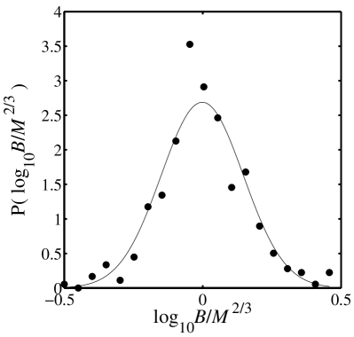
Figure 3: Fluctuations in metabolic rate for mammals with $M\leq 10$ kg taken from Heusner’s data set (heusner91, ). The scaling function $f$ (see equation (2)) is fitted with a lognormal distribution. Values of $B$ have been renormalized as $B/M^{2/3}$ and partitioned into 20 bins.

IV Hypothesis tests

We now construct two types of hypothesis tests to determine whether or not $\alpha=2/3$ or $\alpha=3/4$ should be rejected by the available data. The first test is the standard method of testing the results of a linear regression against a presumed slope. The second is a natural extension of examining fluctuations about a linear fit as per the previous section. By analyzing the correlations of the residuals from the best fit line we are able to quantitatively determine which values of $\alpha$ are compatible with the data. In both tests, we reject an hypothesis when $p<0.01$.

IV.1 Comparison to a fixed $\alpha$

For a given set of $N$ measurements for both mass, $M_{i}$, and metabolic rate, $B_{i}$, we pose the following hypotheses:

$$H_{0}:\alpha = \alpha^{\prime},$$ (3)

$$H_{1}:\alpha \neq \alpha^{\prime}.$$ (4)

We test the null hypothesis, $H_{0}$, in the specific cases $\alpha^{\prime}=2/3$ and $\alpha^{\prime}=3/4$ for data from Kleiber (kleiber32, ), Brody (brody45, ), Bennett and Harvey (bennett87, ), and Heusner (heusner91, ), over various mass ranges. Here, the $p$-value represents the probability that, given two variables linearly related with slope $\alpha^{\prime}$ and subject to Gaussian fluctuations, a data set formed with $N$ samples would have a measured slope $\alpha$ differing at least by $|\alpha-\alpha^{\prime}|$ from $\alpha^{\prime}$ (degroot1975, ). For a null hypothesis with $\alpha=\alpha^{\prime}$, we write the $p$-value as $p_{\alpha^{\prime}}$, e.g., $p_{3/4}$.

For mammals with $M\leq 10$ kg, the results of the hypothesis test are contained in Table 5. The null hypothesis that $\alpha=3/4$ is rejected for both Brody and Heusner’s data and should not be rejected in the case of Kleiber. The alternative null hypothesis that $\alpha=2/3$ is not rejected for both Heusner and Kleiber and rejected in the case of Brody. Again, divisions into mass ranges are somewhat arbitrary and are chosen to help demonstrate the mass-dependence of $\alpha$. For example, for mammals with $M<1$ kg, Brody’s data implies we should not reject the hypothesis that $\alpha=2/3$.

	$N$	$\alpha$	$\sigma(\alpha)$	$p_{2/3}$	$p_{3/4}$
Kleiber	5	0.667	0.016	0.99	0.088
Brody	26	0.709	0.020	$<10^{-3}$	$<10^{-3}$
Heusner	357	0.668	0.010	0.91	$<10^{-15}$

Table 5: Hypothesis test based on standard comparison between slopes that $\alpha=2/3$ and $\alpha=3/4$ for mammals with $M\leq 10$ kg. Here, $\alpha$ is the measured exponent, $\sigma$ is the standard error, and the $p$-values $p_{2/3}$ and $p_{3/4}$ for the hypothesis $\alpha=2/3$ and $\alpha=3/4$ are listed in the last two columns.

Table 6 details results for mammals with $M\geq 10$ kg. In the smaller data sets of Kleiber and Brody the hypothesis that $\alpha=3/4$ is not rejected while for the larger data set of Heusner, $\alpha=3/4$ is rejected. In all cases the hypothesis that $\alpha=2/3$ for large mammals is rejected. Even though Brody and Kleiber’s data sets are consistent with an exponent $\alpha>3/4$, the relative lack of metabolic measurements on large mammals and the strong rejection by Heusner’s larger sample prevents us from drawing definitive conclusions about the particular value, if any, of $\alpha$ for $M\geq 10$ kg.

	$N$	$\alpha$	$\sigma(\alpha)$	$p_{2/3}$	$p_{3/4}$
Kleiber	8	0.754	0.021	$<10^{-4}$	0.66
Brody	9	0.760	0.038	$<10^{-3}$	0.56
Heusner	34	0.877	0.088	$<10^{-12}$	$<10^{-7}$

Table 6: Hypothesis test based on standard comparison between slopes that $\alpha=2/3$ and $\alpha=3/4$ for mammals with $M\geq 10$ kg. See Table 5 for the definition of all quantities.

When all mass ranges are considered for both birds and mammals the hypothesis test (see Table 7) demonstrates that both $\alpha=2/3$ and $\alpha=3/4$ are rejected based on the empirical data on mammals, while $\alpha=2/3$ is not rejected and $\alpha=3/4$ is rejected based on the empirical data on birds. In summary, we find that a single exponent may be appropriate for rough estimates but, from a statistical point of view, it appears that no single exponent explains the data on metabolic scaling for mammals.

	$N$	$\alpha$	$\sigma(\alpha)$	$p_{2/3}$	$p_{3/4}$
Kleiber	13	0.738	0.007	$<10^{-6}$	0.11
Brody	35	0.718	0.011	$<10^{-4}$	$<10^{-2}$
Heusner	391	0.710	0.008	$<10^{-6}$	$<10^{-5}$
Bennett and Harvey	398	0.664	0.007	0.69	$<10^{-15}$

Table 7: Hypothesis test based on standard comparison between slopes that $\alpha=2/3$ and $\alpha=3/4$ for birds and mammals over their entire mass range. See Table 5 for the definition of all quantities.

IV.2 Analysis of residuals

As per our discussion of fluctuations, a sensitive test of a null hypothesis is to check the rank-correlation coefficient of the residuals. In order to test the hypothesis, $\alpha=\alpha^{\prime}$, we pose the following hypotheses:

$$H_{0}:r_{s,\alpha^{\prime}}(z_{i},M_{i}) = 0,$$ (5)

$$H_{1}:r_{s,\alpha^{\prime}}(z_{i},M_{i}) \neq 0.$$ (6)

where the $z_{i}$ are the residuals. The hypothesis $H_{0}$ means that if the residuals for the power law $B=cM^{\alpha^{\prime}}$ are uncorrelated with $M$ then $\alpha^{\prime}$ could be the underlying exponent. The alternative hypothesis $H_{1}$ means that the residual correlations are significant and the null hypothesis should be rejected. The $p$-values represent the probability that the magnitude of the correlation of the residuals, $|r_{s,\alpha^{\prime}}(z_{i},M_{i})|$, would be at least its value as expected for samples taken from randomly generated numbers.

In this case we have tested the hypothesis for a range of exponents, $\alpha^{\prime}=0.6$–$0.8$, and calculated the significance levels for both mammal and bird data compiled by Heusner (heusner91, ) and Bennett and Harvey (bennett87, ), over different mass ranges. The results of this hypothesis test for Heusner’s data is contained in Figure 4 and for Bennett and Harvey’s data in Figure 5. Both tests show that the hypothesis $\alpha=3/4$ is rejected while that of $\alpha=2/3$ is not rejected over all mass ranges considered for both birds and mammals. This does not mean that $\alpha=2/3$ is the “real” exponent, but rather that it, unlike $\alpha=3/4$, is not incompatible with the data.

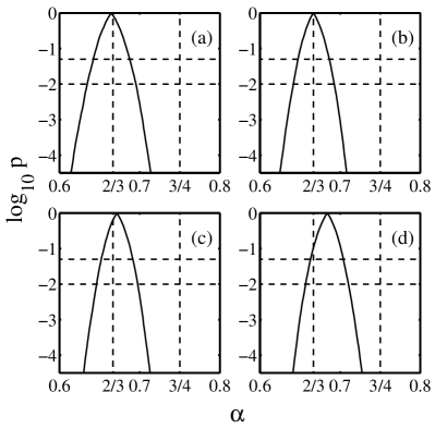
Figure 4: Test of the null hypothesis $H_{0}:r_{s,\alpha^{\prime}}(z_{i},M_{i})=0$ based on mammalian data from Heusner (heusner91, ) (see equation (5)). Shown are plots of $p(\alpha)$ for differing mass ranges. In all plots the two dashed horizontal lines correspond to $p=0.05$ and $p=0.01$. The individual plots correspond to the following ranges: (a) $M<3.2$ kg, (b) $M<10$ kg, (c) $M<32$ kg, (d) all mammals. For all mass ranges considered, $p_{2/3}>0.05$ and $p_{3/4}\ll 10^{-4}$.

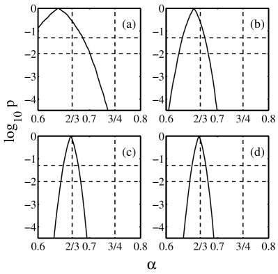
Figure 5: Test of the null hypothesis $H_{0}:r_{s,\alpha^{\prime}}(z_{i},M_{i})=0$ based on bird data from Bennett and Harvey (bennett87, ) (see Figure 4 for details). Here, the individual plots correspond to the following ranges: (a) $M<0.1$ kg, (b) $M<1$ kg, (c) $M<10$ kg, (d) all birds. As for the mammal data, $p_{2/3}>0.05$ and $p_{3/4}\ll 10^{-4}$ for all mass ranges considered.

V Theories

Thus far we have presented empirical evidence that $\alpha$ is mass dependent and that the null hypothesis $\alpha=2/3$ should not be rejected for mammals with $M<10$ kg and all birds in most available data sets. What then of theoretical attempts to derive the 3/4-law of metabolism? We show below that many of these arguments, while often elegant in conception and based on simple physics and geometry, contain sufficient flaws to render them unconvincing for the rejection of the simplest theoretical hypothesis, $\alpha=2/3$.

V.1 Dimensional analysis

Dimensional analysis is a very useful technique when there is only one mass, length, and time scale in a given problem. However in the case of metabolic scaling in biological organisms there has been a long history of theoretical debates over which scales to use when predicting the scaling of metabolic rate via dimensional analysis.

Theories of biological and elastic similarities have been used to explain many structural aspects of organisms such as the length and width of major limbs (gunther82, ; economos82, ; gunther85, ). Using the principles of elastic similarity, Bonner and McMahon (bonner83, ) have tried to explain why quarter-power scaling in body lengths and widths should lead to $\alpha=3/4$. Cross-sections of limbs are argued to scale as $M^{3/4}$ and therefore the power required to move scales in the same way. However, it is not clear why the power output of muscles should be the dominant factor in the scaling of basal metabolic rate. Furthermore, such quarter-power scaling for animal shape is not generally observed (calder84, ).

Recent debates have focused on deriving $\alpha$ solely from dimensional analysis (heusner82a, ; feldman95, ). The problem with all attempts to derive metabolic rate from dimensional analysis is that different constraints lead to different choices of contributing scales (feldman95, ). Explaining the scaling of metabolic rate is therefore displaced to biological questions of energetic constraints, mass density, physiological time, and diffusion constants across surfaces.

V.2 Nutrient Supply Networks

Interest in Kleiber’s law resurged with the suggestion by West, Brown and Enquist (WBE) (west97, ) that nutrient-supplying networks might be the ubiquitous limiting factor in organismal form. This remains an appealing and elegant idea and stands as one of the boldest and most significant attempts at discerning the underlying physical mechanisms responsible for quarter-power scaling. Although previous work had addressed the problem of optimal network structure (cohn54a, ; cohn54b, ; rashevsky62, ; mlabarbera90, ), theoretical relations between optimal networks and the scaling of basal metabolic rate had never been considered.

The basic assumptions of WBE are i) homoiotherms have evolved to minimize the rate at which they dissipate energy; ii) the relevant energy dissipation arises from transport through nutrient-supply networks; iii) these networks are space-filling; and iv) all homoiotherms possess capillaries invariant in size. From these four assumptions WBE derive three important conclusions: i) nutrient-supply networks are fractal; ii) these networks contain area-preserving branching; and iii) metabolic rate scales with $\alpha=3/4$. However, as we show below and in Appendices A and B, the arguments used are mathematically incorrect and as a consequence none of the above conclusions may be derived from the explicit assumptions. Nevertheless, we find the model appealing and potentially useful in understanding a number of biological issues. Thus we detail below where the errors lie to illuminate the path of future work. For clarity, we use the same notation as WBE. For each level $k$ in the network hierarchy one has $N_{k}$ vessels each with length $l_{k}$ and radius $r_{k}$ with $k=1$ being the aorta and $k=N$ being the capillary level. Related important quantities are $n_{k}$, $\gamma_{k}$ and $\beta_{k}$, the ratios of number, length and radius from levels $k-1$ to $k$.

Central to the theory is the connection of these network ratios to metabolic rate. WBE find that $n_{k}=n$, $\beta_{k}=\beta$ and $\gamma_{k}=\gamma$ are all constants independent of $k$ and that

$$\alpha=-\frac{\log n}{\log\gamma\beta^{2}}.$$ (7)

This depends in part on an assumption, which we discuss below, that $B\propto N_{c}$ where $N_{c}$ is the number of capillaries. They also conclude that

$$\beta=n^{-1/2}\qquad\mbox{and}\qquad\gamma=n^{-1/3},$$ (8)

which gives $\alpha=3/4$ in equation (7). Whereas we show below that these relations do not arise from an optimization principle, they do have simple interpretations. The first relation corresponds to networks being area-preserving via $N_{k}r_{k}^{2}=N_{k-1}r_{k-1}^{2}$. The second relation follows from a space-filling criterion that $N_{k}l_{k}^{3}=N_{k-1}l_{k-1}^{3}$. Whether or not space-filling networks satisfy these conditions has been discussed by Turcotte et al. (turcotte98, ), who consider the more general case of side-branching networks and arrive at an equivalent statement of equation (7) where the network ratios $\beta$ and $\gamma$ are to be determined empirically as functions of $n$.

WBE minimize energy dissipation rate by minimizing network impedance using a Lagrange multiplier method. Two types of impedance are considered: Poiseuille flow (lamb45, ) and, for the case of mammals and birds, a more realistic pulsatile flow (womersley55a, ).

We use the Poiseuille case to demonstrate how fractality is not proven by the minimization procedure. The impedance is given by

$$Z=\sum_{k=0}^{N}\frac{8\mu l_{k}}{\pi r_{k}^{4}N_{k}}=\sum_{k=0}^{N}Z_{k}$$ (9)

where $Z_{k}$ is the effective impedance of the $k$th level. As WBE show, the equations are consistent and $Z$ is minimized when

$$\gamma_{k}=\beta_{k}=n_{k}^{-1/3}.$$ (10)

However, the calculations do not require these ratios to be level-independent, and as a consequence, the network need not be fractal. Further details may be found in Appendix A. To see why this is true, we observe that equations (9) and (10) give

$$Z_{k}=\gamma_{k}\beta_{k}^{-4}n_{k}^{-1}Z_{k-1}=1\cdot Z_{k-1}.$$ (11)

Thus, $Z$, the quantity being minimized, is invariant as long as $\gamma_{k}\beta_{k}^{-4}n_{k}^{-1}=1$ for each $k$. This shows that in this setting, a network can have $n_{k}$ varying with $k$ and still be “efficient.” A finding of fractal networks would have provided a derivation of Murray’s empirical law which essentially states that $\beta=n^{-1/3}$ for the outer reaches of the cardiovascular system (murray26, ).

Regardless of these issues, the assumption of Poiseuille flow leads to an approximate metabolic scaling law with $\alpha=1$. WBE suggest that modeling pulsatile flow will provide the explanation for $\alpha=3/4$. The impedance now takes the form

$$Z\propto\sum_{k=0}^{N}\frac{h_{k}^{1/2}}{\sqrt{2}\pi r_{k}^{5/2}N_{k}},$$ (12)

where $h_{k}$ is the thickness of the vessel wall. However, as explained in Appendix B, the equations given by the Lagrange multiplier technique are inconsistent. For example, the equations give $h_{k}=-r_{k}/5$ which means negative wall thicknesses for blood vessels when they are by definition positive (womersley55a, ; womersley55b, ). If reasonable modifications are made to circumvent this issue, then the equations lead to $\alpha=6/7$ rather than $\alpha=3/4$.

In order to obtain the scaling $\alpha=3/4$ one could abandon the minimization calculation and assume a fractal, space-filling, area-preserving network where $B\propto N_{c}$. In support of such an assumption, there is good empirical evidence that blood systems are well approximated by fractals (zamir83, ; fung90, ; kassab93a, ; kassab93b, ). With regards to the assumption that $B\propto N_{c}$, direct measurements for capillary density ($N_{c}/M\propto M^{\alpha-1}$) are reported by Hoppeler et al. (hoppeler81, ) with exponents for the scaling of capillary density across species ranging from $-0.21\pm 0.04$ to $-0.07\pm 0.11$ for various regions of muscle. These numbers are in keeping with higher exponents for the scaling of $N_{c}$ with $M$ in the range 0.75–1.00, but whether or not $B\propto N_{c}$ is itself an unproven assumption. It is probably more likely that the number of capillaries scales with the maximum metabolic rate which is thought to scale with an exponent closer to unity (bishop99, ). At rest not all capillaries diffuse oxygen simultaneously and the limiting factor for basal metabolic rate might not be $N_{c}$.

A simpler and more recent theory based on the idea of networks has been proposed by Banavar et al. (banavar99, ). Here, networks fill $D$-dimensional hypercubes that have $L^{D}$ uniformly distributed transfer sites. The theory is applied to both three-dimensional organisms and two-dimensional river networks. For organisms, Banavar et al. find blood volume scales as $V_{b}\propto L^{(D+1)}$. Since Banavar et al. further assume that $B\propto L^{D}$ and that $V_{b}\propto M$, they conclude that $B\propto M^{D/(D+1)}$. Thus, when $D=3$, this gives $\alpha=3/4$.

However, transfer sites are assumed to be invariant in size and hence $L^{D}$ appears to be proportional to volume $V$ consequently $M$. Thus, both the scalings $V_{b}\propto M$ and $V_{b}\propto M^{(D+1)/D}$ are used, creating an apparent inconsistency. The scaling of the distance between transfer sites and the distinction between Euclidean and non-Euclidean length scales could possibly be clarified to help resolve the dilemma. Note that $V_{b}\propto M$ is supported empirically (stahl67, ).

V.3 Four-dimensional biology

Over two decades ago it was suggested by Blum (blum77, ) that $\alpha=3/4$ could be understood by appealing to a surface law of metabolism in a four-dimensional space. In $d$ dimensions, the “area” $A$ of the hypersurface enclosing a $d$-dimensional hypervolume scales like $A\propto V^{\frac{d-1}{d}}$. When $d=4$, $A\propto V^{3/4}$, although how this could be reconciled with our three-dimensional world was not explained and the theory has been refuted elsewhere (speakman90, ).

Recently, an attempt by West et al. (west99, ) has been made to refine and generalize their earlier work on metabolic scaling (west97, ) using an optimization procedure to explain how an effective fourth dimension could yield $\alpha=3/4$. The idea put forward is that organisms have evolved to maximize the scaling of the effective surface area, $a$, across which resources are exchanged. The area $a$ and the biological volume $v$ are shown to satisfy the relation

$$a\propto v^{(2+\epsilon_{a})/(3+\epsilon_{v})},$$ (13)

where $\epsilon_{a}$ and $\epsilon_{v}$ are exponents to be determined by optimization. West et al. then introduce the relationship $v=al$ where $l$ is a characteristic length of the organism. With the further assumption that $v\propto M$, equation (13) then becomes

$$a\propto M^{(2+\epsilon_{a})/(3+\epsilon_{a}+\epsilon_{l})},$$ (14)

where $\epsilon_{l}=\epsilon_{v}-\epsilon_{a}$. With the conditions that $0\leq\epsilon_{l},\epsilon_{a}\leq 1$, West et al. find that $\epsilon_{a}=1$ and $\epsilon_{l}=0$. Equation (14) then yields $a\propto M^{3/4}$. Assuming $a\propto B$, this gives $\alpha=3/4$.

However, this result contradicts the geometric fact that transfer area can maximally scale as volume, i.e., $a\propto v$, which gives $\alpha=1$. Indeed, this result is obtained by optimizing equation (13) instead of equation (14). Doing so leads to $\epsilon_{a}=1$ and $\epsilon_{v}=0$, assuming $0\leq\epsilon_{a},\epsilon_{v}\leq 1$, which gives $a\propto M$, i.e., $\alpha=1$. In order to reconcile this with the results of West et al., we note that the bounds $0\leq\epsilon_{l},\epsilon_{a},\epsilon_{v}\leq 1$ are overly restrictive. For example, $\epsilon_{l}=-1$ corresponds to the relevant length $l$ being invariant with respect to $M$ and, in this case, equation (14) then gives the same scaling as (13), namely, $a\propto M$. Thus, the contradiction is resolved and the optimization procedure is seen to yield $\alpha=1$ rather than $\alpha=3/4$.

VI Discussion

The possibility that there might be a simple law to explain the scaling of metabolic rates still captures the imagination of many seeking to understand what Kleiber called “the fire of life” (kleiber61, ). It is perhaps for this reason that so many researchers, theorists and empiricists alike, have struggled to deduce explanations for the deviations from the simplest expectation that $\alpha=2/3$.

The shift from $\alpha=2/3$ to $\alpha=3/4$ began with the early work by Kleiber and Brody who found $\alpha\simeq$ 0.72–0.73 in limited data sets (kleiber32, ; brody45, ). Afterwards it was work by Hemmingsen (hemmingsen60, ) and a general consensus among practitioners (blaxter65, ) that simple fractions would be a more convenient standard that led to the widespread acceptance of $\alpha=3/4$. Subsequently, $\alpha=3/4$ has often been taken as fact despite the absence of a comprehensive theory and contradictory evidence from large literature surveys. Most prominent among these surveys are those by Bartels (bartels82, ), Bennett and Harvey (bennett87, ), and Heusner (heusner91, ), which suggest that $\alpha$ depends on body size and taxonomic level.

We have re-analyzed some of the most influential empirical data sets in the study of metabolic rate scaling. We have constructed a set of hypothesis tests which show that in the data sets of Kleiber, Brody, Bennett and Harvey, and Heusner, pure $3/4$-law scaling is not present. For both mammals with $M\leq 10$ kg and all birds we are unable to reject the null hypothesis $\alpha=2/3$. For mammals with $M\geq 10$ kg, systematic deviations from $\alpha=2/3$ appear to be present in all of the data sets, the roots of which might simply be a consequence of a change in body shape for large mammals or might point to a greater evolutionary advantage of large mammals.

We have also reviewed historic and recent attempts to justify $\alpha=3/4$ theoretically. Many of the early efforts to explain the scaling of metabolic rates via dimensional analysis and other crude scaling techniques have been dismissed in the past. Although recent attempts to link metabolic rates to network structure are noteworthy they do not prove the stated conclusions. Nonetheless, we believe that research exploring the role of geometric form and the dynamics of growth in constraining the behavior of networks might lead to important progress in organismal biology.

Stated simply, after a systematic review of the available empirical data and theoretical arguments, we find no compelling evidence of a simple scaling law for metabolic rate, and if it were to exist, we also find no compelling evidence that the exponent should be $\alpha=3/4$.

Appendix A Network optimization calculation for Poiseuille flow

We follow the conventions of WBE and consider the case of Poiseuille flow as a means to derive Murray’s law and the fractal nature of nutrient supply networks. The impedance of the network is

$$Z=\sum_{k=0}^{N}\frac{8\mu l_{k}}{\pi r_{k}^{4}N_{k}}.$$ (15)

Minimizing the network’s impedance with the Lagrange constraints of fixed mass and blood volume along with the assumption of a space filling network leads to the auxiliary function,

$$F_{m}(r_{k},l_{k},N_{k},M)=\sum_{k=0}^{N}\frac{8\mu l_{k}}{\pi r_{k}^{4}N_{k}}$$ (16)

$$+ \lambda\sum_{k=0}^{N}\pi r_{k}^{2}l_{k}N_{k}+\sum_{k=0}^{N}\lambda_{k}N_{k}l_{k}^{3}+\lambda_{M}M.$$

Taking partial derivatives with respect to $l_{j}$, $r_{j}$ and $N_{j}$ we respectively have

$$\frac{\partial F_{m}}{\partial l_{j}} = \frac{8\mu}{\pi r_{j}^{4}N_{j}}+\lambda\pi r_{j}^{2}N_{j}+3\lambda_{j}N_{j}l_{j}^{\,2}=0,$$ (17)

$$\frac{\partial F_{m}}{\partial r_{j}} = \frac{-4\cdot 8\mu l_{j}}{\pi r_{j}^{5}N_{j}}+\lambda 2\pi r_{j}l_{j}N_{j}=0,$$ (18)

and

$$\frac{\partial F_{m}}{\partial N_{j}} = \frac{-1\cdot 8\mu l_{j}}{\pi r_{j}^{4}N_{j}^{2}}+\lambda\pi r_{j}^{2}l_{j}+\lambda_{j}l_{j}^{\,3}=0.$$ (19)

Considering first equation (18), we obtain

$$\lambda=\frac{16\mu}{\pi^{2}r_{j}^{6}N_{j}^{2}}.$$ (20)

Since this holds for all $j$ then

$$1=\frac{16\mu}{\pi^{2}r_{j-1}^{6}N_{j-1}^{2}}\frac{\pi^{2}r_{j}^{6}N_{j}^{2}}{16\mu}=\beta_{j}^{\,6}n_{j}^{2},$$ (21)

where $\beta_{j}=r_{j}/r_{j-1}$ and $n_{j}=N_{j}/N_{j-1}$ which demonstrates that

$$\beta_{j}=n_{j}^{-1/3},$$ (22)

giving us Murray’s law (murray26, ).

After rearranging equation (17) we obtain

$$\lambda_{j} =-\frac{8\mu}{3\pi r_{j}^{4}N_{j}^{2}l_{j}^{\,2}}-\frac{\lambda\pi r_{j}^{2}}{3l_{j}^{\,2}}$$

$$=-\frac{8\mu}{3\pi r_{j}^{4}N_{j}^{2}l_{j}^{\,2}}-\frac{16\mu}{3\pi r_{j}^{4}N_{j}^{2}l_{j}^{\,2}}$$

$$=-\frac{8\mu}{\pi r_{j}^{4}N_{j}^{2}l_{j}^{\,2}},$$ (23)

where we have used the form for $\lambda$ obtained in equation (20). Note that derivatives with respect to $N_{j}$, equation (19), yield the same expression for $\lambda_{j}$ given above:

$$\lambda_{j} =-\frac{-1\cdot 8\mu}{\pi r_{j}^{4}N_{j}^{2}l_{j}^{\,2}}-\frac{\lambda\pi r_{j}^{2}}{l_{j}^{\,2}}$$

$$=\frac{8\mu}{\pi r_{j}^{4}N_{j}^{2}l_{j}^{\,2}}-\frac{16\mu}{\pi r_{j}^{4}N_{j}^{2}l_{j}^{\,2}}$$

$$=-\frac{8\mu}{\pi r_{j}^{4}N_{j}^{2}l_{j}^{\,2}}$$ (24)

The three equations (17), (18) and (19) are therefore consistent but redundant. The redundancy can be seen to lie in the fact that the auxiliary function $F_{m}$ in equation (16) can be written in terms of only two variables for each level $k$: $\xi_{k}=N_{k}l_{k}^{\,3}$ and $\zeta_{k}=r_{k}/l_{k}$. Equation (16) thus becomes

$$F_{m}(\xi_{k},\zeta_{k},M)=\sum_{k=0}^{N}\frac{8\mu}{\pi\zeta_{k}^{4}\xi_{k}}$$ (25)

$$+ \lambda\sum_{k=0}^{N}\pi\zeta_{k}^{2}\xi_{k}+\sum_{k=0}^{N}\lambda_{k}\xi_{k}+\lambda_{M}M.$$

Thus one is only able to obtain information such as ratios of variables rather than exact values for network parameters.

The scaling of length ratios are explicitly determined by WBE’s space-filling assumption

$$N_{k}l_{k}^{\,3}=C.$$ (26)

Thus, even without implementing the minimization procedure the space-filling assumption implies

$$\gamma_{k}=n_{k}^{-1/3},$$ (27)

where $\gamma_{k}=l_{k}/l_{k-1}$ is the length ratio. Finally, the equations (22), (23) (or  (24)) and (27) combine to give

$$\frac{\lambda_{k}}{\lambda_{k-1}} = \frac{r_{k-1}^{4}N_{k-1}^{2}l_{k-1}^{\,2}}{r_{k}^{4}N_{k}^{2}l_{k}^{\,2}}$$ (28)

$$= \beta_{k}^{-4}n_{k}^{-2}\gamma_{k}^{-2}$$

$$= (n_{k}^{-1/3})^{-4}n_{k}^{-2}(n_{k}^{-1/3})^{-2}=1$$

so we have $\lambda_{k}=\lambda_{0}$ for all $k$.

The calculations are seen to be consistent and yield Murray’s law (murray26, ). Variations with respect to $M$ are more subtle since $N=N(M)$ and provide higher order corrections. However, one of WBE’s crucial results, $n_{k}=n$, i.e. that the network is fractal, has not been reproduced. One way to see this is to consider the impedance as impedances in series:

$$Z=\sum_{k=0}^{N}Z_{k}\ \ \mbox{where}\ \ Z_{k}=\frac{8\mu l_{k}}{\pi r_{k}^{4}N_{k}}.$$ (29)

Using equations (22) and (27) we have that

$$\frac{Z_{k}}{Z_{k-1}}=\frac{r_{k-1}^{4}N_{k-1}l_{k}}{r_{k}^{4}N_{k}l_{k-1}}=\frac{\gamma_{k}}{\beta_{k}^{4}n_{k}}=\frac{n_{k}^{-1/3}}{(n_{k}^{-1/3})^{4}n_{k}}=1.$$ (30)

In other words, the same impedance appears at each level. So

$$Z=(N+1)Z_{N}\simeq NZ_{N}=N\frac{8\mu l_{c}}{\pi r_{c}^{4}N_{c}}\propto\frac{N}{N_{c}},$$ (31)

since $r_{c}$ and $l_{c}$ are assumed to be independent of mass and $N_{c}$ is the number of capillaries. This is true regardless of whether or not the structure is fractal. The network has to possess branching ratios that collectively maintain the same impedance from level to level (i.e., $\gamma_{k}/\beta_{k}^{4}n_{k}=1$ as per equation (30)) but there is no requirement that the individual ratios $\gamma_{k}$, $\beta_{k}$ and $n_{k}$ be independent of level. Moreover, without the result that the network is fractal, this minimization procedure no longer yields the power law scaling of metabolic rate (see equation (7)).

Appendix B Network optimization calculation for pulsatile flow

In the case of Poiseuille flow, WBE find a network structure where area preservation is not satisfied ($\beta_{k}\neq n_{k}^{-1/2}$) and, effectively, $\alpha=1$ (if $n_{k}=n$ is assumed). The intended fix is to properly treat pulsatile flow of mammalian blood circulation systems. By doing so we should obtain $\beta_{k}=n_{k}^{-1/2}$ and $\gamma_{k}=n_{k}^{-1/3}$. Together with the assumption $n_{k}=n$, this leads to the conclusion, $N_{c}\propto M^{3/4}$, and assuming $B\propto N_{c}$, it would imply a $3/4$-law of metabolic scaling.

The calculation relies on the results of Womersley’s work on pulsatile flow (womersley55a, ; womersley55b, ). Womersley’s calculations lead to a modification of the Poiseuille impedance. For large tubes one has

$$Z\simeq\frac{\rho c_{0}}{\pi r^{2}}.$$ (32)

where $c_{o}=(Eh/2\rho r)^{1/2}$ is the Korteweg-Moens velocity, $E$ is Young’s modulus, $h$ is the thickness of the vessel wall, $\rho$ is blood density and $r$ is, as before, the vessel radius (womersley55a, ; womersley55b, ). This impedance appears to be per unit length but it has the correct dimensions showing that for a flow with pulsatile forcing in an elastic tube, the impedance is independent of the tube length.

Womersley’s impedance suggests a new auxiliary function:

$$F_{w}(r_{k},h_{k},l_{k},N_{k},M)=\sum_{k=0}^{N}\frac{(Eh_{k}\rho)^{1/2}}{\sqrt{2}\pi r_{k}^{5/2}N_{k}}\\ +\lambda\sum_{k=0}^{N}\pi(r_{k}+h_{k})^{2}l_{k}N_{k}+\sum_{k=0}^{N}\lambda_{k}N_{k}l_{k}^{3}+\lambda_{M}M.$$ (33)

Note that the extra variable of wall thickness, $h_{k}$, has been included in the second term to make it a measure of the total volume taken up by the blood system. The variable $h_{k}$ must appear in the constraints if the minimization is to make any sense and the blood volume is the only reasonable choice—the blood volume constraint becomes a network volume constraint.

On considering variations of equation (33) with respect to $r_{j}$ and $h_{j}$ we obtain

$$\frac{\partial F_{w}}{\partial r_{j}}=-\frac{5}{2}\frac{(Eh_{j}\rho)^{1/2}}{\sqrt{2}\pi r_{j}^{7/2}N_{j}}+\lambda 2\pi(r_{j}+h_{j})l_{j}N_{j}=0,$$ (34)

and

$$\frac{\partial F_{w}}{\partial h_{j}}=\frac{1}{2}\frac{(E\rho)^{1/2}}{\sqrt{2}\pi h_{j}^{1/2}r_{j}^{5/2}N_{j}}+\lambda 2\pi(r_{j}+h_{j})l_{j}N_{j}=0.$$ (35)

Since the second term of these equations are the same we then have an equality between the first terms which simplifies to show that

$$h_{j}=-\frac{1}{5}r_{j}.$$ (36)

This suggests that $r_{k}$ is the distance to the outer wall of blood vessels. We are then measuring the blood volume as before and we should have had $(r_{k}-h_{k})$ instead of $(r_{k}+h_{k})$ in the auxiliary function. However it is apparent from Womersley’s work (womersley55a, ; womersley55b, ) that $r$ is the radius as measured from the center to the inner wall of a blood vessel rather than the outer wall. There appears to be no reasonable and simple way of including the $h_{k}$ into a constraint function and we have an ill-posed problem.

Nevertheless, we may proceed with the calculation by adding an extra assumption that $h_{k}=a_{0}r_{k}$ where $a_{0}>0$. The modified version of equation (34) now gives $\lambda$ as

$$\lambda=\frac{(a_{0}E\rho)^{1/2}}{\sqrt{2}\pi^{2}(1+a_{0})^{2}r_{j}^{4}N_{j}^{2}l_{j}}.$$ (37)

Since the right hand side is independent of $j$ we must therefore have

$$\beta_{j}^{4}n_{j}^{2}\gamma_{j}=1,$$ (38)

and given the space-filling constraint, $\gamma_{j}=n_{j}^{-1/3}$, we obtain

$$1=\beta_{j}^{4}n_{j}^{2}n_{j}^{-1/3}=\beta_{j}^{4}n_{j}^{5/3},$$ (39)

which gives a relationship between the radius and number ratios that is not area-preserving:

$$\beta_{j}=n_{j}^{-5/12}.$$ (40)

A further complication here is that the equations obtained by setting $\partial F_{w}/\partial l_{j}=0$ and $\partial F_{w}/\partial N_{j}=0$ are not consistent.

As in the case of Poiseuille flow, $n_{k}=n$ is not derivable. Assuming that $n_{k}=n$ and using equation (7) we find that the metabolic exponent should be

$$\alpha=-\frac{\ln n}{\ln\gamma\beta^{2}}=-\frac{\ln n}{\ln n^{-1/3}n^{-10/12}}=6/7,$$ (41)

as opposed to the stated $3/4$.

Note that if we had found $\beta_{k}=n_{k}^{1/2}$ then the $3/4$ law would have been deduced (again, assuming $n_{k}=n$). Another observation here is that if the Womersley impedance is taken together with $\beta_{k}=n_{k}^{-1/2}$ then we find that the minimum total impedance is obtained irrespective of the ratios $n_{k}$ being equal or not. So, in the cases of Poiseuille and pulsatile flow a fractal network is not necessary for energy dissipation to be minimized. Additionally, in the case of a pulsatile flow network, $\alpha=3/4$ cannot be derived from the optimization problem as stated. It may instead be derived by assuming an area preserving, space-filling, fractal network where $B\propto N_{c}$.

References

- (1) J. T. Bonner and T. A. McMahon. On Size and Life. Scientific American Library, New York, 1983.
- (2) W. A. Calder III. Size, Function and Life History. Dover, New York, 1996.
- (3) M. Kleiber. Body size and metabolism. Hilgardia, 6:315–353, 1932.
- (4) M. Kleiber. The Fire of Life. An Introduction to Animal Energetics. Wiley, New York, 1961.
- (5) R. Peters. The Ecological Implications of Body Size. Cambridge University Press, Cambridge, 1983.
- (6) K. Schmidt-Nielsen. Scaling: Why is Animal Size So Important? Cambridge University Press, UK, 1984.
- (7) B. J. Anderson, A. D. McKee, and N. H. G. Holford. Size, myths, and the clinical pharmacokinetics of analgesia in paediatric patients. Clinical Pharmacokinetics, 33:313–27, 1997.
- (8) J. Mordenti. Man versus beast: pharmacokinetic scaling in mammals. Journal of Pharmaceutical Sciences, 75:1028–1040, 1986.
- (9) I. Mahmood. Allometric issues in drug development. Journal of Pharmaceutical Sciences, 88:1101–6, 1999.
- (10) I. Burger and J. Johnson. Dogs large and small: the allometry of energy requirements within a single species. J. Nutr., 121(11 (Suppl)):S18–21, 1991.
- (11) J. Cunningham. A reanalysis of the factors influencing basal metabolic rate in normal adults. Am. J. Clin. Nutr., 33:2372–2374, 1980.
- (12) R. Pike and M. Brown. Nutrition an integrated approach. John Wiley and Sons, New York, 1984.
- (13) J. Damuth. Population density and body size in mammalas. Nature, 290:699–700, April 1981.
- (14) S. L. Lindstedt, B. J. Miller, and S. W. Buskirk. Home range, time, and body size in mammals. Ecology, 67(2):413–418, 1986.
- (15) C. Carbone, G. Mace, C. Roberts, and D. Macdonald. Energetic constraints on the diet of terrestial carnivores. Nature, 402:286–8, 1999.
- (16) A. E. Economos. Elastic and/or geometric similarity in mammalian design. J. Theor. Biol., 103:167–172, 1983.
- (17) H. Feldman. The 3/4 mass exponent for energy metabolism is not a statistical artifact. Respir. Physiol., 52:149–163, 1983.
- (18) H. A. Feldman. On the allometric mass exponent, when it exists. J. Theor. Biol., 172:187–197, 1995.
- (19) A. Heusner. Energy metabolism and body size. I. Is the 0.75 mass exponent of Kleiber a statistical artifact? Respir. Physiol., 48:1–12, 1982.
- (20) J. Prothero. Scaling of standard energy-metabolism in mammals: I. Neglect of circadian-rhythms. J. Theor. Biol., 106(1):1–8, 1984.
- (21) K. L. Blaxter, editor. Energy Metabolism; Proceedings of the 3rd symposium held at Troon, Scotland, May 1964. Academic Press, New York, 1965.
- (22) G. B. West, J. H. Brown, and B. J. Enquist. A general model for the origin of allometric scaling laws in biology. Science, 276:122–126, April 1997.
- (23) A. Hemmingsen. Energy metabolism as related to body size and respiratory surfaces, and its evolution. Rep. Steno Mem. Hosp., 9:1–110, 1960.
- (24) A. Heusner. What does the power function reveal about structure and function in animals of different size? Ann. Rev. Phsyiol., 49:121–133, 1987.
- (25) M. Rubner. Ueber den einfluss der körpergrösse auf stoffund kraftwechsel. Z. Biol., 19:535–562, 1883.
- (26) S. Brody. Bioenergetics and Growth. Reinhold, New York, 1945.
- (27) Kleiber’s motivation in part was to make calculations less cumbersome with a slide rule (see p. 59 in schmidt-nielsen84 ).
- (28) A. A. Heusner. Size and power in mammals. J. Exp. Biol., 160:25–54, 1991.
- (29) P. Bennett and P. Harvey. Active and resting metabolism in birds—allometry, phylogeny and ecology. J. Zool., 213:327–363, 1987.
- (30) H. Bartels. Metabolic rate of mammals equals the 0.75 power of their body weight. Exp. Biol. and Medicine, 7:1–11, 1982.
- (31) A. C. Economos. On the origin of biological similarity. J. Theor. Biol., 94:25–60, 1982.
- (32) B. Gunther. Theories of biological similarities—30 years of trial and error. Arch. Biol. Med. Exp., 18(3–4):197–224, 1985.
- (33) B. Gunther and E. Morgado. Dimensional analysis and theory of biological similarity. Exp. Biol. Med., 7:12–20, 1982.
- (34) A. Heusner. Energy metabolism and body size. II. Dimensional analysis and energetic non-similarity. Respir. Physiol., 48:13–25, 1982.
- (35) J. J. Blum. On the geometry of four-dimensions and the relationship between metabolism and body mass. J. Theor. Biol., 64:599–601, 1977.
- (36) G. B. West, J. H. Brown, and B. J. Enquist. The fourth dimension of life; fractal geometry and allometric scaling of organisms. Nature, 284:1677–1679, 1999.
- (37) J. R. Banavar, A. Maritan, and A. Rinaldo. Size and form in efficient transportation networks. Nature, 399:130–132, May 1999.
- (38) W. H. Press, S. A. Teukolsky, W. T. Vetterling, and B. P. Flannery. Numerical Recipes in C. Cambridge University Press, second edition, 1992.
- (39) A. Heusner. Body mass, maintenance and basal metabolism in dogs. J. Nutr., 121(11 Suppl):S8–17, Nov. 1991.
- (40) W. Jungers, editor. Size and scaling in primate biology. Advances in Primatology. Plenum Press, New York, 1985.
- (41) J. M. Allman. Evolving brains. Scientific American Library, New York, 1999.
- (42) Following Bennett and Harvey bennett87 , we take one sample for each species of bird selecting those with lowest mass-specific resting metabolic rate. Note that we also include organisms that Bennett and Harvey state were measured during their active cycle whereas Bennett and Harvey do not. The use of other selection criteria does not greatly affect the results we present here.
- (43) R. C. Lasiewski and W. R. Dawson. A re-examination of the relation between standard metabolic rate and body weight in birds. Condor, 69:13–23, 1967.
- (44) S. C. Kendeigh, V. R. Dol’nik, and V. M. Gavrilov. Avian energetics. In J. Pinowski and S. Kendeigh, editors, Granivorous birds in ecosystems, pages 129–204, 363–73, Cambridge, 1977. Cambridge University Press.
- (45) J. Prothero. Scaling of energy-metabolism in unicellular organisms—a reanalysis. Comp. Biochem. Physiol. A-Physiol., 83(2):243–248, 1986.
- (46) M. Patterson. A mass-transfer explanation of metabolic scaling relations in some aquatic invertebrates and algae. Science, 255(5050):1421–1423, 1992.
- (47) M. Patterson. Correction. Science, 256(5058):722–722, 1992.
- (48) J. Kinnear and G. Brown. Minimum heart rates of marsupials. Nature, 215:1501, 1967.
- (49) P. S. Dodds and D. H. Rothman. Geometry of river networks I: Scaling, fluctuations, and deviations. Submitted to Phys. Rev. E, 2000.
- (50) M. H. DeGroot. Probability and Statistics. Addison-Wesley, Reading, Massachusetts, 1975.
- (51) T. Hastie and R. Tibshirani. Generalized additive models: Some applications. J. Amer. Stat. Assoc., 82:371–86, 1987.
- (52) D. Cohn. Optimal systems I. The vascular system. Bull. Math. Biophys., 16:59–74, 1954.
- (53) D. Cohn. Optimal systems II. The vascular system. Bull. Math. Biophys., 17:219–227, 1955.
- (54) N. Rashevsky. General mathematical principles in biology. In N. Raschevsky, editor, Physicomathematical Aspects of Biology, Proceedings of the International School of Physics “Enrico Fermi”; course 16, pages 493–524, New York, 1962. Academic Press.
- (55) M. LaBarbera. Principles of design of fluid transport systems in zoology. Science, 249:992–1000, 1990.
- (56) D. L. Turcotte, J. D. Pelletier, and W. I. Newman. Networks with side branching in biology. J. Theor. Biol., 193:577–592, 1998.
- (57) H. Lamb. Hydrodynamics. Dover, New York, 6th edition, 1945.
- (58) J. R. Womersley. Method for the calculation of velocity, rate of flow and viscous drag in arteries when the pressure gradient is known. J. Physiol., 127:553–563, 1955.
- (59) C. D. Murray. The physiological principle of minimum work. I. The vascular system and the cost of blood volume. Proc. Natl. Acad. Sci. U.S.A, 12:207–214, 1926.
- (60) J. R. Womersley. Oscillatory motion of a viscous liquid in a thin-walled elastic tube—I: The linear approximation for long waves. Phil. Mag., 46(373):199–221, 1955.
- (61) Y.-C. B. Fung. Biomechanics: motion, flow, stress, and growth. Springer-Verlag, New York, 1990.
- (62) G. S. Kassab, C. A. Rider, T. N. J., and Y. B. Fung. Morphometry of pig coronary arterial trees. Am. J. Physiol., 265:H350–H365, 1993.
- (63) K. Kassab, G. S. Imoto, F. C. White, C. A. Rider, Y.-C. B. Fung, and C. M. Bloor. Coronary arterial tree remodeling in right ventricular hypertropy. Am. J. Physiol., 265:H366–H375, 1993.
- (64) M. Zamir, S. M. Wrigley, and B. L. Langille. Arterial bifurcations in the cardiovascular system of a rat. J. Gen. Physiol., 81:325–335, 1983.
- (65) H. Hoppeler, O. Mathieu, E. Weibel, R. Krauer, S. Lindstedt, and C. Taylor. Design of mammalian respiratory system VIII. Capillaries in skeletal muscles. Respir. Physiol., 44:129–150, 1981.
- (66) C. M. Bishop. The maximum oxygen consumption and aerobic scope of birds and mammals: getting to the heart of the matter. Proc. Roy. Lond. B., 266:2275–81, 1999.
- (67) W. R. Stahl. Scaling of respiratory variables in mammals. Journal of Applied Physiology, 22:453–460, 1967.
- (68) J. Speakman. On Blum’s four-dimensional geometric explanation for the 0.75 exponent in metabolic allometry. J. Theor. Biol., 144(1):139–141, 1990.