Theory of periodic swarming of bacteria: application to Proteus mirabilis

Abstract

The periodic swarming of bacteria is one of the simplest examples for pattern formation produced by the self-organized collective behavior of a large number of organisms. In the spectacular colonies of Proteus mirabilis (the most common species exhibiting this type of growth) a series of concentric rings are developed as the bacteria multiply and swarm following a scenario periodically repeating itself. We have developed a theoretical description for this process in order to get a deeper insight into some of the typical processes governing the phenomena in systems of many interacting living units.

Our approach is based on simple assumptions directly related to the latest experimental observations on colony formation under various conditions. The corresponding one-dimensional model consists of two coupled differential equations investigated here both by numerical integrations and by analysing the various expressions obtained from these equations using a few natural assumptions about the parameters of the model. We have determined the phase diagram corresponding to systems exhibiting periodic swarming and discuss in detail how the various stages of the colony development can be interpreted in our framework. We point out that all of our theoretical results are in excellent agreement with the complete set of available observations. Thus, the present study represents one of the few examples, where self-organized biological pattern formation is understood within a relatively simpe theoretical approach leading to results and predictions fully compatible with experiments.

I Introduction

To gain an insight into the development and dynamics of various multicellular assemblies, we must understand how cellular interactions build up the structure and result in certain functions at the macroscopic, multicellular level. Microorganism colonies are one of the simplest systems consisting of many interacting cells and exhibiting a non-trivial macroscopic behavior. Therefore, a number of recent studies have focussed on experimental and theoretical aspects of colony formation and the related collective behavior of microorganisms [1, 2].

The swarming cycles exhibited by many bacterial species, notably Proteus (P.) mirabilis, have been known for over a century [3]. When Proteus cells are inoculated on the surface of a suitable hard agar medium, they grow as short “vegetative” rods. After a certain time, however, cells start to differentiate at the colony margin into long “swarmer” cells possessing up to 50 times more flagella per unit cell surface area. These swarmer cells migrate rapidly away from the colony until they stop and revert by a series of cell fissions into the vegetative cell form, in a process termed consolidation. The resulting vegetative cells grow normally for a time then swarmer cell differentiation is initiated in the outermost zone (terrace), and the process continues in periodic cycles resulting in a colony with concentric zonation depicted in Fig 1. Similar cyclic behavior has been observed in an increasing number of Gram-negative and Gram-positive genera including Proteus, Vibrio, Serratia, Bacillus and Clostridium (for reviews see [4, 5, 6]).

The reproducibility and regularity of swarming cycles together with the finding that its occurrence is not limited to a single species suggest that periodic swarming phenomena can be understood and quantitatively explained on the basis of mathematical models. In this manuscript we first give an overview of the relevant experimental findings related to the swarming of P. mirabilis, then construct a simple model with two limit densities. We then investigate the behavior of the model as a function of the control parameters and compare it to experimental results.

II Overview of experimental findings

a Differentiation.

As reviewed in [5, 6], the differentiation of vegetative cells is accompanied by specific biochemical changes. Swarmer cells enhance the synthesis of flagellar proteins, extracellular polysaccharides, proteases and virulence factors, while exhibit reduced overall protein and nucleic acid synthesis and oxygen uptake. These findings may be explained by arguing that the production and operation of flagella is expensive and may require the repression of non-essential biosynthetic pathways. The largely (10-30 fold) elongated swarmer cells develop by a specific inhibition of cell fission which seems not affecting the doubling time of the cell mass or DNA.

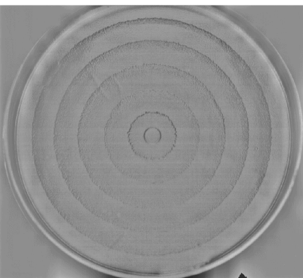
FIG. 1.: Typical Proteus mirabilis colony. It was grown on the surface of a 2.0% agar substrate for two days. The inner diameter of petri-dish is 8.8 cm. Gray shades are proportional to the cell density: the cyclic modulation is apparent.

The differentiation process is initiated by a number of external stimuli including specific signalling molecules and physico-chemical parameters of the environment. As an example for the latter, the viscosity of the surrounding medium is presumably sensed by the hampered rotation of the flagella [7, 8]. Neither the signal molecules that initiate the differentiation nor the involved intracellular signalling pathways are identified yet, but a corresponding transmembrane receptor has been found recently [9]. The structure of this receptor, together with other findings reviewed in [6], suggest a ‘quorum sensing’ regulatory pathway [10] characteristic for many, cell density dependent collective bacterial behaviors like sporulation, luminescence, production of antibiotics or virulence factors[11].

b Migration of swarmer cells.

It is well established [5] that swarmer cell migration does not require exogenous nutrient sources, since swarmer cells replated onto media devoid of nutrients continue to migrate normally. The ability of migration depends on the local swarmer cell density as isolated single swarmer cells cannot move, while a group of them can. It was also demonstrated [12] that the mechanism by which bacteria swarm outwards involved neither repulsive nor attractive chemotaxis. The typical swimming velocity (i.e., in liquid environment) of swarmer cells is $\approx 100$mm/h [13] which is also their maximal swarming speed and rate of colony expansion on soft agar plates [5]. In the usual experimental conditions for investigating swarming colony formation the front advances with a speed of $0.5-10$ mm/h [14, 9, 15, 13]. Unfortunately, in these cases there is no information available on the velocity of individual swarmer cells, but it must be between the colony expansion speed and the swimming velocity.

c Consolidation.

The molecular mechanisms of consolidation, i.e., the downregulation of the gene activity responsible for swarming behavior [16] is even less known than that of differentiation. If the swarming motility utilizes intracellular energy reserves as has been suggested [5], then swarmer cells must have a finite lifetime. In addition to the septation of swarmer cells taking place at the outermost terrace, inside the colony the differentiation process, i.e., the supply of fresh swarmer cells must also be shut off. The cessation of swarmer cell production does not seem to be due to severe nutrient depletion since vegetative cells keep growing (although with decreasing growth rate) well inside the colony for many hours after the last swarmer cells were produced in that region [14].

d Colony formation.

The cycle time (total length of the migration and consolidation periods) has been found [14] to be rather stable ($\approx 4h$) for a wide range of nutrient and agar content of the medium. The size of the terraces and the duration of the migration phases were strongly influenced (up to an order of magnitude, and up to a factor of 3, respectively) by the agar hardness. The nutrient concentration did not have an observable effect on these quantities from $0.01\%$ up to $1\%$ glucose concentrations. There was, however a remarkable positive correlation between the cycle time and the doubling time (ranging from $0.7$h up to $1.8$h) of the cells.

Two interfacing colonies inoculated with a time difference of a few hours and therefore being in different phases of the migration-consolidation cycle, were found to maintain their characteristic phases [14, 15]. Thus, the control of the swarming cycle must be sufficiently local.

e Cycle rescheduling.

A few experiments investigated the cell density dependence of the duration of quiescent growth (lag phase) prior to the first migration phase. These studies clearly revealed that vegetative cells have to reach a threshold density to initiate swarming [14, 15], in accord with the suggested quorum sensing molecular pathway of the initiation of swarmer cell differentiation.

Agar cutting experiments demonstrated that a cut inside the inner terraces does not influence the swarming activity [15]. However, when the cut has been made just behind the swarming front, the duration of the swarming phase was shortened and consolidation was lengthened by up to $40\%$ [15].

Even more interestingly, mechanical mixing of the cell populations before the expected beginning of consolidation expands the duration of the swarming phase considerably, by up to $50\%$[13]. This finding, together with replica-printing experiments[13] demonstrates that at the beginning of the consolidation phase still a large pool of swarmer cells exists and seems to be “trapped” at the rear of the outermost terrace.

III The model

Taking into account the above described experimental findings, here we construct a model which is capable of explaining most of the observed features of colony expansion through swarming cycles.

(i) The model is based on the vegetative and swarmer cell population densities only, denoted by $\rho^{o}$ and $\rho^{*}$, respectively. These values are defined on the basis of cell mass instead of cell number, therefore one unit of swarmer cells is transformed into one unit of vegetative cells during consolidation.

(ii) Vegetative cells grow and divide with a constant rate $r_{0}\approx 1$h^-1 [14, 15]. This will later allow us to establish a direct correspondence between cell density increase and elapsed time.

(iii) Usually, swarmer cell differentiation is initiated when the local density of the vegetative cells exceeds a threshold value ($\rho^{o}_{min}\approx 10^{-2}$ cells/$\mu$m² [14, 15]). (Prior the first swarming phase experiments indicate the presence of an extra time period $t_{\ell}$ which is probably associated with the biochemical changes required to develop the ability of the swarming transition. This effect is present only at the seeding of the colony, thus $t_{\ell}=0$ otherwise.) When $\rho^{o}=\rho^{o}_{min}$ at time $t_{0}$, some of the vegetative cells enter the differentiation process, modeled by introducing a rate $r$. Since the biomass production rate is assumed to be unchanged during the differentiation process, the rate of producing new vegetative cells is $r_{0}-r$ and the differentiating cells elongate with the normal growth rate $r_{0}$.

(iv) The full development of swarmer cells, i.e., a typical 20-fold increase in length needs a time ($t_{d}\approx\ln 20/r_{0}\approx 3$h) comparable with, or even longer than the length of a consolidation period, hence can not be neglected. Therefore, the first “real” swarmer cells, which are able to move appear only at $t_{0}+t_{d}$.

(v) The production of swarmer cells is limited in time and the length $\tau$ of the time interval during which vegetative cells can enter the differentiation process is another phenomenological parameter of our model.

As we here focus on the periodicity of colony expansion, we do not consider what happens in the densely populated regions after $t_{0}+\tau$. Specifically, in our model any activity of the vegetative cells ceases in these parts of the system.

(vi) Swarmer cells can migrate only if their density exceeds a threshold density $\rho^{*}_{min}$. Above that threshold, swarmer cells are assumed to move randomly with a diffusion constant $D_{0}$. The finite lifetime of swarmer cells is incorporated into the model through a constant rate ($r^{*}$) decay.

Unfortunately there are no good estimates on these parameters in the literature. According to recent experimental observations [17], $\rho^{*}_{min}$ is less than $10\%$ of the value of $\rho^{o}$ prior the beginning of the swarming phase, i.e., $0.1\rho^{o}_{min}e^{r_{0}t_{d}}\approx 10^{-2}$ cells/$\mu$m². $D_{0}$ may be estimated as $v_{0}^{2}t_{p}/2$ with $v_{0}$ being the typical speed of swarming cells and $t_{p}$ being the persistence time of their motion. As $v_{0}$ is approximately $30$mm/h (see Sec II.b) and $t_{p}$ is in the order of minutes, $D_{0}$ is estimated to be in the order of 10 mm²/h.

The above considerations lead to the following set of equations

$$\dot{\rho}^{o}(t) = r_{0}\rho^{o}(t)+\Gamma(t)-\Gamma^{*}(t)$$ (1)

$$\dot{\rho}^{*}(t) = -\Gamma(t)+\Gamma^{*}(t-t_{d})e^{r_{0}t_{d}}+\nabla D(\rho^{*})\nabla\rho^{*}$$ (2)

where the consolidation ($\Gamma$) and differentiation ($\Gamma^{*}$) terms are given by

$$\Gamma=r^{*}\rho^{*}\hbox{~{}~{}and~{}~{}}\Gamma^{*}=r(\rho^{o},t)\rho^{o}.$$ (3)

FIG. 2.: Schematic representation of the model for swarming colony formation. (a) The two basic quantities are the vegetative and swarmer cell densities, which can be transformed into each other, and changed by proliferation and motility. The dotted lines represent regulatory (threshold) effects: The rate of differentiation is assumed to be dependent on the vegetative cell density, and the motility of swarmer cells is also determined by their local density. (b) Notations and typical time courses of vegetative and swarmer cell densities prior the beginning of the first migration phase. If $t<t_{0}$ the density $\rho$ (or $\rho^{o}$) grows with a constant rate $r_{0}$. After reaching the density threshold $\rho^{o}_{min}$, vegetative cells keep growing only with a rate $r_{0}-r$, but the total density ($\rho$) of the vegetative cells and the differentiating swarmer cells still grows with a rate $r_{0}$. After the time required for the full elongation of a swarmer cell (when $\rho$ reaches $\rho_{min}$), $\rho^{*}$ becomes positive, and for $r^{*}=0$ asymptotically would grow with a rate $r$.

Eqs. (2) can be significantly further simplified by making use of the possibility to measure elapsed time with the increase in $\rho^{o}$. In particular, neglecting correction terms related to consolidation in areas where $\rho^{o}>\rho^{o}_{min}$, i.e., where primarily differentiation takes place, we can cast $\Gamma^{*}(t-t_{d})e^{r_{0}t_{d}}$ in the form

$$r\rho^{o}(t-t_{d})e^{r_{0}t_{d}}=r\rho^{o}_{min}e^{(r_{0}-r)(t-t_{d}-t_{0})}e^{r_{0}t_{d}}=$$ (4)

$$r\rho^{o}_{min}e^{r_{0}(t-t_{0})}e^{-r(t-t_{0}-t_{d})}=r\rho^{o}(t)e^{rt_{d}}$$ (5)

for $t>t_{0}+t_{d}\equiv t_{1}$. Let us introduce a transformed population density $\rho$ as

$$\rho(t)=\left\{\begin{array}[]{ccl}\rho^{o}(t)&\mbox{for~{}~{}}\rho^{o}<\rho^{o}_{min}&\mbox{i.e., for~{}~{}}t<t_{0}\cr\rho^{o}(t)e^{r(t-t_{0})}&\mbox{for~{}~{}}\rho^{o}>\rho^{o}_{0}&\mbox{and~{}~{}}t<t_{1}\cr\rho^{o}(t)e^{rt_{d}}&\mbox{for~{}~{}}\rho^{o}>\rho^{o}_{0}&\mbox{and~{}~{}}t>t_{1}\end{array}\right.$$ (6)

which is in fact the total density of the vegetative and the differentiating, but not yet fully differentiated swarmer cells (see Fig. 2). With this notation, using (5) and similar considerations for $t_{0}<t<t_{0}+t_{d}$, Eqs. (2) can be written into a simple, not retarded form

$$\dot{\rho} = r_{0}\rho+r^{*}\rho^{*}-r(\rho)\rho$$ (7)

$$\dot{\rho}^{*} = -r^{*}\rho^{*}+r(\rho)\rho+\nabla D(\rho^{*})\nabla\rho^{*},$$ (8)

where

$$r(\rho)=\left\{\begin{array}[]{cl}r&\mbox{for~{}~{}}\rho_{min}<\rho<\rho_{max}\cr 0&\mbox{otherwise}\end{array}\right.$$ (9)

with $\rho_{min}=e^{rt_{d}}\rho_{min}\approx 10^{-1}$ cells/$\mu$m² and $\rho_{max}(\tau)=e^{(r_{0}-r)\tau}\rho_{min}$. If the $\Gamma\ll(r_{0}-r)\rho$ condition does not hold in the $[t_{0},t_{1}]$ time interval, then $\rho_{min}$ must be also treated as a dynamical variable. This case will not be considered here. In the following we use $\rho$ for the characterization of vegetative cell density.

IV Results

A Numerical method in 1D

The model defined through Eqs. (8) has the following seven parameters: the rates $r_{0}$, $r$, $r^{*}$, threshold densities $\rho_{min}$, $\rho_{max}$ (or $\tau$), $\rho^{*}_{min}$ and the diffusivity $D_{0}$. However, this number can be reduced to four by casting the equations in a dimensionless form using $1/r_{0}\approx 1$h as time unit, $\rho_{min}\approx 0.1$ cells/$\mu$m² as density unit and $x_{0}=\sqrt{D_{0}/r_{0}}\approx 3$mm as the unit length. The resulting control parameters are $r/r_{0}$, $r^{*}/r_{0}$, $\rho_{max}/\rho_{min}=\exp[(r_{0}-r)\tau]$ and $\rho^{*}_{min}/\rho_{min}$. To obtain continuous density profiles, the step-function dependence of $D$ on $\rho^{*}$ was replaced by

$$D(\rho^{*})={D_{0}\over 2}\left[1+\tanh 2\alpha{\rho^{*}-\rho^{*}_{min}\over\rho^{*}_{min}}\right]$$ (10)

with $\alpha=10$ providing a rather steep, but continuous crossover.

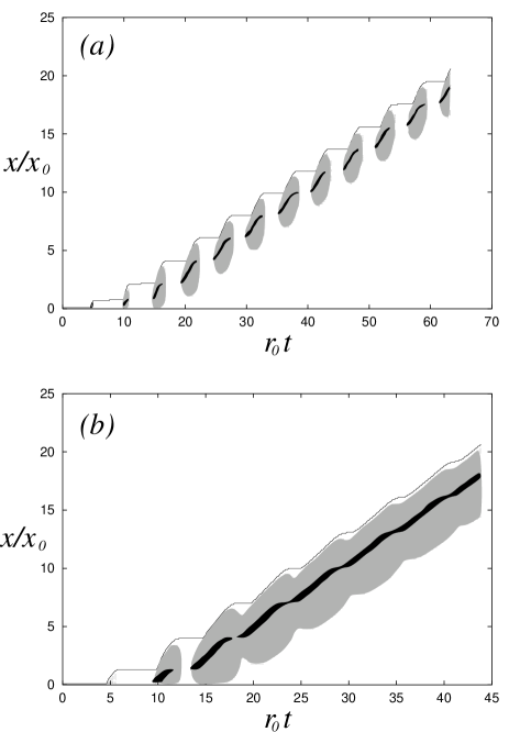
FIG. 3.: Time development of the model obtained by numerical integration of the equations, starting from a localized “inoculum” at $t=0$, $x=0$. The continuous line represent the colony boundary (maximal value of $x$ for which $\rho(x)+\rho^{*}(x)>0$). The filled gray and black areas are regions where swarmer cells are motile, and where swarmer cells are produced, respectively. For $\rho_{max}=1.3$, $\rho^{*}_{min}=0.01$, $r=0.3$ and $r^{*}=1.0$ the expansion of the system is clearly periodic (a). If we increase the production of swarmer cells by increasing $\rho_{max}$ to $2.0$ then the periodicity is gradually lost and a continuous expansion takes place (b).

Representative examples for the time development of the model are shown in Fig. 3. The production of swarmer cells is localized, and determined by the density profile of vegetative cells at the end of migration periods. In this particular model $\rho(x)$ is decreasing towards the colony edge, therefore in the migration phases the source of swarmer cells is moving outwards. The front of swarmer cells is expanding from the inside of the last terrace. Because of the decay term $\Gamma$, cells become non-motile first at the colony edge.

B Phase diagram

Each of the dimensionless control parameters can have an important effect on the dynamics of the system. As an example, if the duration $\tau$ of swarmer cell production is increased, then the consecutive swarming cycles are not separated and a continuous expansion takes place with damped oscillations (Fig. 3b). To map the behavior of the system as a function of the control parameters, the following procedure was applied. Migration periods were identifed by requiring $\max_{x}\rho^{*}(x)>\rho^{*}_{min}$. For a given set of parameters we determined the lengths $\{t_{i}\}$ of the consecutive migration periods, and the system was classified as periodic if the three largest values of the set $\{t_{i}\}$ were the same within $20\%$. Otherwise, the expansion was classified as continuous as long as $\max_{i}\{t_{i}\}$ was large enough: comparable with the total duration of the simulated expansion.

FIG. 4.: Phase diagram of the system as the function of cumulative swarmer cell production density $P$ and migration threshold $\rho^{*}_{min}$ for various values of swarmer cell decay rate $r^{*}$. If the production is high or the motility threshold is low enough then continuous expansion can be observed. On the other hand, if the production is too low or the motility threshold is too high then no expansion takes place. In an intermediate regime periodic growth can be observed. The boundaries of this parameter regime are plotted for $r^{*}/r_{0}=1.0$ (thick continuous line), $0.4$ (thick dashed line) and $0.1$ (thick dotted line). The thin continuous line represent an approximate upper bound (13) for cyclic colony expansion. The insert demonstrates that the fourth parameter of the model, $r$, is irrelevant: for $r^{*}/r_{0}=1$ and $r/r_{0}=0.01$ ($\Box$), $0.3$ ($\circ$), $0.5$ ($\triangle$) and various values of $\rho_{max}$ and $\rho^{*}_{min}$ the type of colony expansion was classified. Open symbols correspond to cyclic growth, filled symbols to continuous growth while dots denote no expansion. Note that the corresponding regions completely overlap irrespectively of the value of $r$.

The behavior of the model is summarized in Fig. 4, where the boundaries of the various regimes are plotted for three different values of $r^{*}/r_{0}$. We found, that $r$ and $\rho_{max}$ can be combined into one relevant parameter, the swarmer cell production density, as

$$P=\int_{-\infty}^{\infty}\Gamma^{*}(x,t)dt={r\over r_{0}-r}(\rho_{max}-\rho_{min}),$$ (11)

which quantity does not depend on the choice of position $x$. As the insert demonstrates, for a given $P$, the actual values of $r$ or $\rho_{max}$ are irrelevant to this kind of classification in the parameter regime investigated. The general structure of the phase diagram was found to be similar for various values of $r^{*}$. For large enough $P$ or low enough $\rho^{*}_{min}$ a continuous expansion takes place, while for too small $P$ or large $\rho^{*}_{min}$ the expansion of the system is finite. For intermediate values of these parameters an oscillating growth develops exhibiting well distinguishable consolidation and migration phases. As the lifetime of the swarmer cells is increased, the parameter regime, in which periodic behavior is exhibited, is shrinked and moved towards lower $P$ values.

One can easily estimate the position of the boundary of the non growing phase based on that (i) the width $w$ of the terraces is small (this assumption is justified later, in Fig. 7.), thus (ii) the time required for the diffusive expansion of the swarmer cells is much shorter than their lifetime, which, in turn, is (iii) shorter than the duration of a swarming cycle: $r^{*}/r_{0}\sim 1$. The amount of swarmer cells produced in one period is $Pw$. Neglecting the decay during expansion, the width $w^{\prime}$ of the next, new terrace can be determined from the conservation of cell number as

$$2\rho^{*}_{min}w^{\prime}=w(P+\rho^{*}_{r}-\rho^{*}_{min}),$$ (12)

where $\rho^{*}_{r}$ denotes the swarmer cell density remaining from the previous swarming cycle and the symmetric expansion of the released swarmers was also taken into account. To achieve a sustainable growth $w^{\prime}\geq w$ is required, resulting in a condition $3\rho^{*}_{min}\leq P+\rho^{*}_{r}$. If $\rho^{*}_{r}\ll P$, as one can expect for $r^{*}/r_{0}\sim 1$, we get for the boundary of the non growing phase

$$P=3\rho^{*}_{min},$$ (13)

which, as Fig. 4 demonstrates, is indeed in good agreement with the numerical data.

C Terrace formation.

The average length $T$ of a full swarming cycle was calculated by determining the position of the peak in the power spectrum of $S(t)=\int_{0}^{\infty}\rho^{*}(x,t)dx$, the time dependence of the total number of swarmer cells in the system. As Fig. 5 demonstrates, the dimensionless cycle time values are widely spread between values of $3$ and $12$. However, $T$ is only sensitive to changes in $r_{0}$, $r^{*}$ and $\rho^{*}_{min}/\rho_{min}$, hence it does not depend on $\rho_{max}$ or $\tau$.

FIG. 5.: The cycle time $T$ as a function of the approximate consolidation rate $r^{*}\rho^{*}_{min}$. The data collapse indicates that the impact on $T$ of the other parameters ($\rho_{max}$ and $r$) is negligible. The various symbols correspond to different values of $r^{*}/r_{0}$ as $0.1$ ($+$), $0.2$ ($\times$), $0.3$ ($\Box$), $0.4$ ($\circ$), $0.5$ ($\triangle$), $0.7$ ($\bigtriangledown$), $1.0$ ($\diamond$). The dashed line is a plot of Eq.(15). Circles mark out the assumed parameter values characteristic of four different P. mirabilis strains.

The average expansion speed $v$ and terrace size $w$ were also calculated in the parameter regime resulting oscillatory expansion of the colony. First we determined the time $t_{1/3}$ when the system reached $1/3$ of its maximal simulated expansion $R_{max}=R(t_{max})$, with $R(t)$ being the position of the expanding colony edge and $t_{max}$ is the total duration of the simulation. The average speed was then calculated for the time interval between $t_{min}=\max(t_{1/3},t_{max}-5T)$ and $t_{max}$: for the last $5T$ long time interval, or for the last $2/3$rd of the total expansion, depending on which was smaller. After obtaining $v$ as $[R_{max}-R(t_{min})]/(t_{max}-t_{min})$, the average terrace width was calculated as $w=vT$. Fig. 6. shows the dependence of these parameters on the swarmer cell production density $P$ and migration density threshold $\rho^{*}_{min}$. In general, decreasing $\rho_{min}^{*}$ or increasing $P$ results in an increase in both $w$ and $v$. As Fig. 7. demonstrates, for a given $r^{*}$, the relevant parameter controlling $w$ is $P/\rho_{min}^{*}$.

The results on the cycle time $T$ (Fig. 5.) can be interpreted as follows. As $\rho^{*}_{min}$ is a good estimate on the density of swarmer cells in the expanding front, at the end of migration phase the vegetative cell density within the new terrace is given by $r^{*}\rho^{*}_{min}T^{*}$ with $T^{*}$ being the duration of the migration phase. Now the length of the consolidation phase, $T-T^{*}$, is determined by the requirement that $\rho$ must reach $\rho_{min}$:

$$\rho_{min}=r^{*}\rho^{*}_{min}T^{*}e^{r_{0}(T-T^{*})}=r^{*}\rho^{*}_{min}{T^{*}\over e^{r_{0}T^{*}}}e^{r_{0}T}.$$ (14)

As $T^{*}\approx 1/r_{0}$, the estimate (14) is simplified to

$$r_{0}T=\ln{r_{0}\rho_{min}e\over r^{*}\rho^{*}_{min}},$$ (15)

which gives a rather accurate fit to the numerically determined data (Fig. 5).

FIG. 6.: Terrace size (a) and expansion speed (b) of the system for $r^{*}/r_{0}=1$ as a function of the dimensionless swarmer cell production density $P$. The connected points correspond to various values of the migration threshold $\rho_{min}^{*}/\rho_{min}$. In general, decreasing $\rho_{min}^{*}$ or increasing $P$ results in an increase in both $w$ and $v$. Only parameters resulting in periodic expansion were investigated. Circles mark out the assumed parameter values characteristic of four different P. mirabilis strains.

FIG. 7.: Terrace size $w$ vs $P/\rho_{min}^{*}$ for various values of $r^{*}/r_{0}$. Note the collapse of the data presented in Fig. 6a. The terrace size vanishes approaching the parameter regime where no sustainable expansion of the system is possible.

D Lag phase

FIG. 8.: (a) Length $T_{L}$ of the lag phase vs the initial inoculum density $\rho_{0}$ for $t_{\ell}=0$, $r_{0}t_{d}=3$ and various values of $r/r_{0}$ (0.3, 0.1, 0.03, 0.01, 0.003 and 0.001). The transition between the regimes separated by $\rho^{o}_{min}$ becomes more smooth for decreasing $r/r_{0}$. (b) The experimentally calculated $r_{0}T_{L}$ values vs the estimated inoculum density (based on 5 mm and 7 mm inoculum droplet sizes for the RPM and BB strains, respectively) and the corresponding fits using Eqs. (16) and (18).

Since the duration ($T_{L}$) of the lag phase (the time period before the first migration phase) has been in the focus of many recent experiments, now we turn our attention towards this quantity. At least four processes determine $T_{L}$. First, there is a time $t_{\ell}$ associated with the biochemical changes required to switch into swarming mode. As discussed in Sec. II.a, these processes take place only prior the first swarming phase, and are presumably related to sensing the altered environmental conditions. Second, the cell population must reach the threshold density $\rho^{o}_{min}$ (at time $t_{0}$). Third, $t_{d}$ time is required to produce fully differentiated swarmer cells (at time $t_{1}$), and finally, the density of the swarmer cells must reach the migration threshold $\rho^{*}_{min}$. Let us investigate how these parameters depend on the initial inoculum density $\rho_{0}$.

As $\rho$ grows with a rate $r_{0}$ until the appearance of swarmer cells,

$$r_{0}t_{1}=\max\left[t_{\ell}+t_{d},\ln(\rho_{min}/\rho_{0})\right].$$ (16)

The time development of $\rho^{*}$ can be estimated by the integration of Eq.(8) with $r^{*}=0$ (i.e., assuming $\Gamma\ll\Gamma^{*}$) yielding

$$\rho^{*}(t+t_{1})={r\over r_{0}-r}\rho_{0}e^{r_{0}t_{1}}[e^{(r_{0}-r)t}-1].$$ (17)

Therefore, $t^{*}=T_{L}-t_{1}$ is given by

$$r_{0}t^{*}={1\over 1-r/r_{0}}\ln\left({r_{0}-r\over r}{\rho^{*}_{min}\over\rho_{0}e^{r_{0}t_{1}}}+1\right),$$ (18)

an expression usually giving a minor correction to $t_{1}$.

Fig. 8a. shows the above calculated $r_{0}T_{L}$ vs $\rho_{0}$ for $t_{\ell}=0$. The increase in length of the swarmer cells was assumed to be $20$-fold, thus $r_{0}t_{d}=\ln 20\approx 3$, which value can be seen for $\rho_{0}\gg\rho_{min}$. In the opposite limit, when $\rho_{0}\ll\rho_{min}$, we have $r_{0}T_{L}\approx-\ln\rho_{0}+const$. These relations allow the determination of both $r_{0}$ and $r$ (using the known value of $\rho_{min}/\rho^{*}_{min}$) from the experimental data on $T_{L}(\rho_{0})$.

E Comparison with experiments

Most of the published experimental data are related to the average period length, $T$ and terrace size $w$. From these parameters the average expansion speed can be calculated as $v=w/T$, i.e., $v$ is not an independent quantity. As we could see in the previous paragraph, from the density dependence of the lag phase the parameters $r_{0}$, $t_{\ell}+t_{d}$ and $r$ can be estimated. Notice that this estimate on $r_{0}$ is in principle different from the value obtained by the usual methods based on densitometry in liquid cultures. Technically, $\rho^{*}_{min}$ could be also determined [14], but such measurements are not published yet.

There are four Proteus strains studied systematically in experiments: the PRM1, PRM2, BB2000 and BB2235 strains (see Table I). To extract the values of the model’s parameters the following procedure was applied. (i) We estimated $r_{0}$ based on lag phase length measurements. (ii) From the calculated $r_{0}T$ values the $\rho^{*}_{min}/\rho_{min}$ ratio was estimated (assuming $r^{*}/r_{0}=1$) based on Eq.(15), see Fig. 5. (iii) Using Eqs. (17) and (18), by a nonlinear fitting procedure (Levenberg-Marquardt method, [18], see Fig. 8b.) $\rho_{min}$, $r$, and $t_{\ell}+t_{d}$ was determined. (The latter value is not relevant in respect the periodicity of the behavior.) (iv) Knowing $\rho^{*}_{min}$ and $\rho_{min}$, from the experimental terrace width data $x_{0}$ and $P$ can be estimated using Fig. 6. (v) Finally, $\tau$ is given by

$$r_{0}\tau=\ln\left({Pr_{0}\over\rho_{min}r}+1\right)$$ (19)

The parameter values of the model are summarized in Table II, together with the predictions on $T$, $v$ and $w$. An excellent agreement can be achieved with biologically relevant parameter values.

Two classes of model parameters should be distinguished: (a) the ones which are related to the growth and differentiation of the cells ($r_{0}$, $r^{*}$, $\rho_{min}$, and $P(r,\tau)$) and (b) those which depend on agar softness ($D_{0}$ and $\rho^{*}_{min}$). For a given strain we expect that a change in the agar concentration influences only the latter group, while changes in temperature may affect both, but primarily $r_{0}$. In fact, as Table I. demonstrates, by changing $D_{0}$ and keeping all the other, growth-related parameters constant, we could quantitatively reproduce the colony behavior observed on various agar concentrations. Similar statement holds for the temperature effects as well, where the only parameter we changed was the growth rate $r_{0}$.

V Discussion

Periodic bacterial growth patterns have been in the focus of research in the last few years. Since a colony can be viewed as a system where diffusing nutrients are converted into diffusing bacteria, one may not be surprised by the emergence of spatial structures [19]. However, the periodic patterns of bacterial colonies are qualitatively different from the Liesegang rings (for a recent review see [20]) developing in reaction-diffusion systems: the spacing between the densely populated areas is uniform and independent of the concentration of the other diffusing species, i.e., the nutrients. The Turing instability is also well-known for producing spatial structures [21], but in that case the pattern emerges simultaneously in the whole system. It is also known, that bacteria can aggregate in steady concentric ring structures as a consequence of chemotactic interactions [22, 23], but as we discussed in Sec. II., it is established that swarming of P. Mirabilis does not involve chemotaxis communication. Therefore, none of the well known generic pattern forming schemes can explain the colony structure of swarming bacteria.

As we mentioned in the introduction, oscillatory growth is also exhibited by other bacterial species. One of them, Bacillus subtilis, has been the subject of systematic studies on colony formation and a number of models have been constructed to explain the observed morphology diagram (for recent reviews see [24, 25]). Only one model addressed the problem of migration and consolidation phases: Mimura et al [26] set up a reaction-diffusion system in which the decay rate of the bacteria was dependent both on their concentration and the locally available amount of nutrients. The periodic behavior is then a consequence of the following cycle: if nutrients are used up locally, then the bacterial density starts to decay preventing the further expansion of the colony. Nutrients diffuse to the colony and accumulate due to the reduced consumption of the already decreased population. The increased nutrient concentration gradually allows the increase in population density and the expansion of the colony, which starts the cycle from the beginning. While this can be a sound explanation for B. subtilis, as we discussed in Sec. II., the nutrient limitation clearly can not explain neither the differentiation nor the consolidation of P. Mirabilis swarmer cells.

Another recent study [27] focused on the swarming of Serratia liquefaciens. In that case the structure of the molecular feedback loops are better explored, and were resolved in the model. The production of a wetting agent was initiated by high concentrations of specific signalling molecules. The colony expansion was considered to be a direct consequence of the flow of the wetting fluid film, in which process the only effect of bacteria (besides the aforementioned production) was changing the effective viscosity of the fluid. The wetting agent production was downregulated through a negative feedback loop involving swarmer cell differentiation. This scenario is certainly not applicable to P. Mirabilis, where swarmer cells actively migrate outwards and their role is quite the opposite: enhancing the expansion of the colony.

The first theoretical analysis focusing on P. mirabilis was performed by Esipov and Shapiro (ES) in [28]. Their model was constructed based on assumptions similar to ours, and could reproduce the alternating migration and consolidation phases during the colony expansion. However, the complexity of the ES model involves a rather large number of model parameters, which practically impedes both the full mapping of the parameter space and the quantitative comparison of the model results with experimental findings. The major differences between our and the ES model can be summarized as follows: (i) we do not resolve the age of the swarmer population. Instead, we have a density measure and a constant decay rate implying an exponential lifetime distribution on the (unresolved) level of individual cells. Since the available microbiological observations [5, 13] suggest only that the lifetime is finite, there is no reason for preferring any specific distribution. (ii) We did not incorporate into our model an unspecified “memory field” with a built-in hysteresis. Instead, we implemented a density-dependent motility of the swarmer cells, which behavior has been indeed observed [4, 5, 6]. (iii) In our model the fully differentiated swarmer cells do not grow, which assumption is probably not fundamental for the reported behavior, but it seems to be more realistic because of the repression of many biosynthetic pathways [5]. Finally, (iv) we do not consider any specific interaction between the motility of swarmer cells and the non-motile vegetative cell population. Although such interactions probably exist, they are undocumented, and as we demonstrated, are not required for the formation of periodic swarming cycles. However, such effects can be important in the actual determination of the density profiles.

With these differences, which are not compromising the biological relevance of the model, we were able to map completely the phase diagram, establish approximate analytical formulas and estimate the value of all model parameters in the case of four different strains. In addition, experimental data measured under various conditions could be explained with one particular parameter setting in the case of the PRM1 strain indicating the predictive power of our approach. Our model is a minimal model in the sense that all of the explicitly considered effects (thresholds, diffusion, etc.) were required to produce the oscillatory behavior, thus, it can not be simplified further. Such minimal models can serve as a comparison baseline for later investigations of various specific interactions.

The values of the microscopic parameters of the model can be either measured directly (like $r_{0}$, $\rho^{*}_{min}$, $\rho_{min}$, $\rho_{max}$ or $r^{*}$) or can be determined indirectly from experimental data (as $\rho_{min}^{o}$ and $r$). Most of these measurements have not yet been performed, we hope that our work will motivate such experiments further examining the validity of our assumptions. In fact, one of the parameters, $r^{*}/r_{0}$ was set to 1 during the fitting processes, as currently there is no available data to estimate its value. Our numerical results suggest that it is probably larger than $0.3$, and it is unlikely to be larger than 2 (meaning an average lifetime less than 30 minutes). Within this range our qualitative conclusions are valid, while the numerical values of the parameter estimates can change up to a factor of $3$.

The behavior of “precocious” swarming mutants reported in [9] deserves special attention. First, we would like to comment on the huge difference found in the value of the transition rate $r$ (see Table II). We emphasize that this is not an arbitrary output of a multiparameter fitting process. First, we have reasons to believe, that the motility thresholds of the two BB strains are rather similar. Knowing the growth rates and the cycle times, Eq. (15) shows us that the difference in the values of $\rho_{min}$ can not exceed one order of magnitude. Assuming then this maximal difference in $\rho_{min}$, $r$ remains the only free variable in Eqs. (16)-(18), and the fitting can be performed unambigously. Thus, we are quite confident that such a large difference exists in $r$ showing that the rsbA gene (in which these strains differ) influences not only the cell density threshold, but the rate of differentiation as well. It is also interesting to note that in Fig. 8b the behavior of the PRM2 and PRM1 strains reflect a relation very similar to that of the BB2000 and BB2235 strains. Finally, our calculations predicted a slightly longer cycle time for the precocious swarming mutant BB2235, which is also in accord with the actual experimental findings (see Fig 2. of [9]).

In our model the assumed functional form of the density-dependence of the diffusion coefficient is somewhat different from the most often considered one [24, 26], namely

$$D(\rho)\sim\rho^{k}.$$ (20)

The advantage of (20) is that it allows analytic solutions for certain cases [21], however, it describes an unlimited, arbitrarily fast diffusion inside the colony where the density is high. In contrast, in real colonies the diffusion of cells is certainly bounded, and the expansion of the boundary can be often limited by the supply of cells from behind [14]. Therefore we believe that our thresholded formulation (10) is a better approximation of what is taking place inside the real colonies.

Finally we would like to comment on the role of nutriens in the swarming behavior of P. mirabilis. In our model there is a phenomenological parameter ($\tau$) determining how long the swarmer cells are produced at a given position in the colony. When investigating the dependence of the cycle time on this parameter, as Fig. 5 demonstrates, we found an extremely weak effect. Thus, at least within the framework of this model there is no contradiction between the assumption that the swarmer cell production ceases due to nutrient (or accumulated waste) limitations, and the seemingly nutrient-independent cyclic behavior. In fact, this idea can be developed further. By increasing $\tau$ (or decreasing the motility threshold $\rho^{*}_{min}$) we arrive into a regime where the migration/consolidation phases are not clearly separable as a motile swarmer cell population exists even when the expansion of the colony is slower. Experiments mapping the morphology diagram of P. mirabilis (Fig. 2 of [29]) showed that there are certain values of agar hardness and nutrient concentration, for which the expansion of the colony is still oscillating, but the periodic density changes are smeared out due to the presence of motile swarmer cells in the consolidation periods. If one associates the increasing agar hardness with increasing $\rho^{*}_{min}$ and the nutrient concentration with $\tau$ then one can qualitatively reproduce those (i.e., the $P_{r}$ and $P_{h}$) regions of the morphology diagram.

Strain				PRM1			PRM2	BB2000	BB2235
Experimental	Temperature	32oC	32oC	32oC	37oC	22oC	32oC	37oC	37oC
condition	Agar	2.0%	2.45%	2.0%	n.a.	n.a.	2.0%	n.a.	n.a.
	Reference	[14]	[14]	[15]	[14]	[14]	[14]	[9]	[9]
	$T$ [h]	4.7	4.7	4.0	3.5	8.5	6.0	3.0	3.1
Colony-level	$v$ [mm/h]	1.7	0.6	1.0	n.a.	n.a.	n.a.	3.3	3.3
	$w$ [mm]	8.0	3.0	3.8	n.a.	n.a.	n.a.	10	10
Cellular-level	$r_{0}$ [1/h]	0.6	0.6	n.a.	1.0	0.4	n.a.	n.a.	n.a.

TABLE I.: Summary of experimental data for four different P. mirabilis strains under various experimental conditions. The value of $r_{0}$ was determined from growth monitoring in liquid cultures.

Strain				PRM1			PRM2	BB2000	BB2235
Experimental	Temperature	32oC	32oC	32oC	37oC	22oC	32oC	37oC	37oC
condition	Agar	2.0%	2.45%	2.0%	n.a.	n.a.	2.0%	n.a.	n.a.
Microscopic	$r_{0}$ [1/h]	0.53∗ (0.6)	0.53∗ (0.6)	0.7∗	1.0	0.4	1.0∗	2.5∗	1.5∗
parameters	$\rho_{min}$ [cell/$\mu$m2]			$0.06$			$0.6$	$2.0$	$0.2$
(independent)	$\rho^{*}_{min}$ [cell/$\mu$m2]			$6\cdot 10^{-3}$			$6\cdot 10^{-3}$	$4\cdot 10^{-3}$	$4\cdot 10^{-3}$
	$\rho_{max}$ [cell/$\mu$m2]			$0.6$			$240$	$3000$	$2.2$
	$r/r_{0}$			$10^{-1}$			$10^{-4}$	$2\cdot 10^{-5}$	$3\cdot 10^{-2}$
	$D_{0}$ [mm2/h]	20	3.2	6	–	–	–	60	40
(derived)	$\rho^{0}_{min}$ [cell/$\mu$m2]			$3\cdot 10^{-3}$			$3\cdot 10^{-2}$	$10^{-1}$	$10^{-2}$
	$P/\rho_{min}$			0.9			0.04	0.03	0.3
	$\tau/T$			0.7			0.9	0.9	0.3
	$\rho^{*}_{min}/\rho_{min}$			$10^{-1}$			$10^{-2}$	$2\cdot 10^{-3}$	$2\cdot 10^{-2}$
	$x_{0}$ [mm]	6	2.3	3.0	–	–	–	5.0	5.0
	$v_{0}$ [mm/h]	50	20	27	–	–	–	85	70
Macroscopic	$T$ [h]	5.5 (4.7)	5.5 (4.7)	4.7 (4.0)	3.3 (3.5)	8.2 (8.5)	5.6 (6.0)	2.9 (3.0)	3.2 (3.1)
behavior	$v$ [mm/h]	1.4 (1.7)	0.5 (0.6)	0.8 (1.0)	n.a.	n.a.	n.a.	3.4 (3.3)	3.1 (3.3)
	$w$ [mm]	7.8 (8.0)	3.0 (3.0)	3.9 (3.8)	n.a.	n.a.	n.a.	10 (10)	10 (10)

TABLE II.: Model parameters and the corresponding results for the strains and experimental conditions specified in Table I. The model has seven microscopic parameters, the rates $r_{0}$, $r$, $r^{*}$, the threshold densities $\rho_{min}$, $\rho^{*}_{min}$ and $\rho_{max}$ and the diffusivity $D_{0}$. For each of the strains $r^{*}=r_{0}$ was assumed. For comparison, other (derived) microscopic parameters are also included. The calculated period lengths, terrace sizes and expansion speeds are also presented together with the corresponding experimental values (in parentheses). The values marked by an asterisk ($*$) were derived from the lag phase length data based on Eqs. (16) and (18). Note the similarity between the PRM1 and BB2235, and also between the PRM2 and BB2000 strains.

REFERENCES

- [1] J. A. Shapiro and M. Dworkin, editors. Bacteria as multicellular organisms. Oxford University Press, Oxford, 1997.
- [2] W. Alt, A. Deutsch, and G. A. Dunn, editors. Dynamics of cell and tissue motion. Birkhäuser, Basel, 1997.
- [3] G. Hauser. Über Fäulnissbacterien und deren Beziehungen zur Septicämie. F. G. W. Vogel, Leipzig, 1885.
- [4] F.D. Williams and R.H. Schwarzhoff. Nature of the swarming phenomenon in Proteus. Ann. Rev. Microbiol., 32:101–122, 1978.
- [5] C. Allison and C. Hughes. Bacterial swarming: an example of procaryotic differentiation and multicellular behaviour. Sci. Progress, 75:403–422, 1991.
- [6] G. M Fraser and C. Hughes. Swarming motility. Cur. Opin. Microbiol., 2:630–635, 1999.
- [7] C. Allison, H-C. Lai, D. Gygi, and C. Hughes. Cell differentiation of Proteus mirabilis is initiated by glutamine, a specific chemoattractant for swarming cells. Mol. Microbiol., 8:53–60, 1993.
- [8] L. McCarter and M. Silvermann. Surface-induced swarmer cell differentiation of Vibrio parahaemolyticus. Mol. Microbiol., 4:1057–1062, 1990.
- [9] R. Belas, R. Schneider, and M. Melch. Characterization of Proteus mirabilis precocious swarming mutants: Identification of rsbA, encoding a regulator of swarming behavior. J. Bacteriol., 180:6126–6139, 1998.
- [10] C. Fuqua, S. C. Winans, and E. P. Greenberg. Census and consensus in bacterial ecosystems: The luxR-luxI family of quorum-sensing transcriptional regulators. Ann. Rev. Microbiol., 50:727–751, 1996.
- [11] J. A. Shapiro. Thinking about bacterial populations as multicellular organisms. Ann. Rev. Microbiol., 52:81–104, 1998.
- [12] F.D. Williams, D. M. Anderson, P. S. Hoffman, R. H. Schwarzhof, and S. Leonard. Evidence against chemotaxis in swarming of Proteus mirabilis. J. Bacteriol., 127:237–248, 1976.
- [13] T. Matsuyama, Y. Takagi, Y. Nakagawa, H. Itoh, J. Wakita, and M. Matsushita. Dynamic aspects of the structured cell population in a swarming colony of Proteus mirabilis. J. Bacteriol., 182:385–393, 2000.
- [14] O. Rauprich, M. Matsushita, C. J. Weijer, F. Siegert, S. E. Esipov, and J. A. Shapiro. Periodic phenomena in Proteus mirabilis swarm colony development. J. Bacteriol., 178:6525–6538, 1996.
- [15] H. Itoh, J.-I. Wakita, T. Matsuyama, and M. Matsushita. Periodic pattern formation of bacterial colonies. J. Phys. Soc. Japan, 68:1436–1443, 1999.
- [16] A. Dufour, R. B. Furness, and C. Hughes. Novel genes that upregulate the Proteus mirabilis flhDC master operon controlling flagellar biogenesis and swarming. Mol. Microbiol., 29:741–751, 1998.
- [17] M. Matsushita, unpublished results.
- [18] W.H. Press, S.A. Teukolsky, W.T. Vetterling, and B.P. Flannery. Numerical Recipes, 2nd edition. Cambridge University Press, Cambridge, 1992.
- [19] M.C. Cross and P.C. Hohenberg. Pattern formation outside of equilibrium. Rev. Mod. Phys., 65:2, 1993.
- [20] T. Antal, M. Droz, J. Magnin, Z. Rácz, and M. Zrinyi. Derivation of the Matalon-Packter law for Liesegang patterns. J. Chem. Phys., 109:9479–9486, 1998.
- [21] J. D. Murray. Mathematical Biology. Springer Verlag, Berlin, 1989.
- [22] L. Tsimring, H. Levine, I. Aranson, E. Ben-Jacob, I. Cohen, O. Shochet, and W.. N. Reynolds. Aggregation patterns in stressed bacteria. Phys. Rev. Lett., 75:1859–1862, 1995.
- [23] D.E Woodward, R. Tyson, M.R. Myerscough, J.D. Murray, E.O. Budrene, and H.C. Berg. Spatio-temporal patterns generated by Salmonella typhimurium. Biophys. J., 68:2181, 1995.
- [24] I. Golding, Y. Kozlovsky, I. Cohen, and E. Ben-Jacob. Studies of bacterial branching growth using reaction-diffusion models for colonial development. Physica A, 260:510–554, 1998.
- [25] M. Matsushita, J. Wakita, H. Itoh, K. Watanabe, T. Arai, T. Matsuyama, H. Sakaguchi, and M. Mimura. Formation of colony patterns by a bacterial cell population. Physica A, 274:190–199, 1999.
- [26] M. Mimura, H. Sakaguchi, and M. Matsushita. Reaction-diffusion modelling of bacterial colony patterns. Presented first at the Kyoto Conference on Math. Biol, 1996; Physica A, 282:283–303, 2000.
- [27] M.A. Bees, P. Andresen, E. Mosekilde, and M. Giskov. The interaction of thin-film flow, bacterial swarming and cell differentiation in colonies of Serratia liquefaciens. J. Math. Biol., 40:27–63, 2000.
- [28] S.E. Esipov and J.A. Shapiro. Kinetic model of Proteus mirabilis swarm colony development. J. Math. Biol., 36:249–268, 1998.
- [29] A. Nakahara, Y. Shimada, J. Wakita, M. Matsushita, and T. Matsuyama. Morphological diversity of the colony produced by bacteria Proteus mirabilis. J. Phys. Soc. Japan, 65:2700–2706, 1996.