Loading a vapor cell magneto-optic trap using light-induced atom desorption

Abstract

Low intensity white light was used to increase the loading rate of ⁸⁷Rb atoms into a vapor cell magneto-optic trap by inducing non-thermal desorption of Rb atoms from the stainless steel walls of the vapor cell. An increased Rb partial pressure reached a new equilibrium value in less than 10 seconds after switching on the broadband light source. After the source was turned off, the partial pressure returned to its previous value in $1/e$ times as short as 10 seconds.

PACS number(s): 32.80.Pj, 42.50.Vk, 68.45.Da

I Introduction

The evaporative cooling techniques used to achieve Bose-Einstein condensation in atomic gases [2, 3, 4, 5] rely on loading large numbers of atoms into magnetic traps with long trap lifetimes. The approach originally taken by Anderson et al. [2] was to load Rb atoms into a vapor cell [6] magneto-optic trap (MOT) [7] and to subsequently transfer atoms into a magnetic trap located in the same cell. Large numbers of atoms and long lifetimes were achieved by optimizing the Rb partial pressure and by working with long MOT loading times.

We have found a simple way to improve such a setup by modulating the vapor pressure such that it is high for initial trap loading and then low again in order to achieve long lifetimes in a magnetic trap. The technique requires the use of a white light source (WLS) with radiation incident upon the inner walls of the vapor cell. When such a light source is turned on, Rb atoms that coat the inner walls of the stainless steel vacuum chamber are quickly desorbed and the Rb vapor pressure suddenly increases. The vapor pressure soon returns to equilibrium after the WLS is turned off. This enables loading large numbers of atoms into the MOT in a relatively short amount of time, while preserving the low pressures required for long magnetic trap lifetimes. The WLS method that we describe here is a possible alternative to the double-chamber techniques [8] and Zeeman slowing techniques [3, 4] currently used to capture atoms before evaporatively cooling in a magnetic trap. In our experiments, the WLS method is used in the manner described here for the achievement of BEC in a vapor cell, where the WLS frees us from environmentally induced variations in vapor pressure; for example, regardless of chamber temperature, we can load large numbers of atoms into our MOT and achieve BEC [9].

Light-induced atom desorption (LIAD) has previously been used to obtain optically thick Na and Rb vapors in cells made of glass, pyrex, and sapphire [10, 11]. In most of these experiments, the inner walls of the vapor cells were coated with paraffin or silane in order to enhance the LIAD efficiency by reducing the alkali atom adsorption energy [12]. In our work, an optically thick vapor was not required. Since we did not need desorption rates characteristic of coated cells, we could desorb atoms directly from stainless steel.

II Background

We first review the basic mechanisms involved in the operation of a vapor cell MOT, lucidly described in Ref. [6], in order to understand the gains available with the LIAD method. In a vapor cell MOT, atoms are loaded into the MOT at a rate $R$. This rate depends upon the size and intensity of the laser cooling and trapping beams and the Rb partial pressure. Atoms with velocities below a critical velocity will be captured by the trap. Atoms are also lost from the trap due to collisions, limiting the number that can be loaded into the MOT. The rate equation for the number, $N$, of trapped atoms is given by

$$\frac{dN}{dt}=R-N\left(\frac{1}{\tau_{\mbox{{b}}}}+\frac{1}{\tau_{\mbox{{Rb}}}}\right)-\beta\int n^{2}dV,$$ (1)

where $1/\tau_{\mbox{{b}}}$ is the trap loss rate due to collisions with background gas atoms and $1/\tau_{\mbox{{Rb}}}$ is the loss rate determined by collisions with untrapped Rb atoms. The trap density, $n$ in the volume integral, contributes to density-dependent losses within the trap with a loss coefficient of $\beta$. The loss rate $1/\tau_{\mbox{{b}}}$ is proportional to the pressure of the background gas, and like $R$, $1/\tau_{\mbox{{Rb}}}$ is proportional to the Rb partial pressure. In the absence of density-dependent collisional losses ($\beta=0$) [13], and with a Rb partial pressure that is much higher than the background pressure ($1/\tau_{\mbox{{Rb}}}\gg 1/\tau_{\mbox{{b}}}$), the rate equation becomes

$$\frac{dN}{dt}=R-\frac{N}{\tau_{\mbox{{Rb}}}}.$$ (2)

The limiting number, $N_{\mbox{{lim}}}$, that can be loaded into the MOT is obtained when the increase in number due to loading balances the loss due to collisions. At this point, $N=N_{\mbox{{lim}}}$ and $dN/dt=0$, yielding

$$N_{\mbox{{lim}}}=R\tau_{\mbox{{Rb}}},$$ (3)

independent of the Rb partial pressure [6].

Frequently, the background-gas collisions can not be neglected, and the total number reached will be less than $N_{\mbox{{lim}}}$. The maximum number $N_{\mbox{{max}}}$ that can be captured for a given Rb partial pressure will then be given by

$$N_{\mbox{{max}}}=N_{\mbox{{lim}}}\frac{\tau_{\mbox{{MOT}}}}{\tau_{\mbox{{Rb}}}}=R\tau_{\mbox{{MOT}}},$$ (4)

where

$$\frac{1}{\tau_{\mbox{{MOT}}}}=\frac{1}{\tau_{\mbox{{b}}}}+\frac{1}{\tau_{\mbox{{Rb}}}}.$$ (5)

If the trap starts filling at time $t=0$, the number of atoms in the MOT at any point in time is given by

$$N(t)=N_{\mbox{{max}}}\left[1-\exp{\left(-\frac{t}{\tau_{\mbox{{MOT}}}}\right)}\right].$$ (6)

Because of the appearance of $\tau_{\mbox{{MOT}}}$ as the time constant in the exponential, we define $\tau_{\mbox{{MOT}}}$ as the ”MOT loading time.”

The lifetime of a magnetic trap in the same chamber also depends upon the collision rate of trapped atoms with background atoms. Thus the magnetic trap lifetime $\tau$ is proportional to $\tau_{\mbox{{MOT}}}$. We express this proportionality as $\tau=\tau_{\mbox{{MOT}}}/\alpha$, where for our traps, $\alpha\sim 4$. For evaporative cooling experiments, where large numbers of atoms and long magnetic trap lifetimes are both necessary, the product of total number $N_{\mbox{{max}}}$ and magnetic trap lifetime is the critical parameter to maximize [14]. Because of the relationship between $\tau$ and $\tau_{\mbox{{MOT}}}$, we can alternatively view this requirement as maximizing the product of $N_{\mbox{{max}}}$ and $\tau_{\mbox{{MOT}}}$. We must therefore find the optimum Rb partial pressure for a given background pressure. Multiplying Eq. 4 by $\tau_{\mbox{{MOT}}}$ leads to maximization of $\tau_{\mbox{{MOT}}}^{2}/\tau_{\mbox{{b}}}$ ($N_{\mbox{{lim}}}$ is independent of vapor pressure). Under optimal conditions, with constant Rb partial pressure, $N_{\mbox{{max}}}\tau_{\mbox{{MOT}}}$ is maximized for $\tau_{\mbox{{b}}}=\tau_{\mbox{{Rb}}}=\tau_{\mbox{{MOT}}}/2$ and hence $N_{\mbox{{max}}}=N_{\mbox{{lim}}}/2$ and $N_{\mbox{{max}}}\tau_{\mbox{{MOT}}}=N_{\mbox{{lim}}}\tau_{\mbox{{b}}}/4$.

However, we can further improve the number-lifetime product (which from now on we will generally designate as $N\tau$) by permitting a modulation of the Rb vapor pressure. If the Rb partial pressure is temporarily increased until the trap contains the maximum possible number of atoms ($N=N_{\mbox{{max}}}=N_{\mbox{{lim}}}$), at which point the Rb vapor is suddenly reduced to a negligible level ($\tau_{\mbox{{MOT}}}\sim\tau_{\mbox{{b}}}$), an increase of a factor of 4 in $N\tau$ will be realized. Furthermore, the time needed to load the MOT is significantly shortened when $\tau_{\mbox{{Rb}}}\ll\tau_{\mbox{{b}}}$ during the loading interval, increasing the repetition rate of the experiment.

The goal of our experiment was to realize gains in $N\tau$ by modulating the Rb vapor pressure in the described manner with the white light source, thus improving conditions for evaporative cooling and obtaining BEC.

III Experimental setup and measurement techniques

Our stainless steel vacuum chamber consisted of a vapor cell atom trapping chamber with indium-sealed windows, a liquid nitrogen-filled cold finger which protruded into the chamber, and a Rb cold finger at $0^{\circ}$C, as shown in Fig. 1. The vacuum in the chamber was maintained by a Ti-sublimation pump and an ion pump. We maintained a Rb vapor in the chamber by slightly opening a valve between the chamber and a Rb cold finger. This replenished Rb that was pumped out of the chamber.

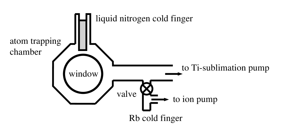
FIG. 1.: An illustration of our apparatus. The MOT was formed in the atom trapping chamber, and the WLS light entered into the chamber through a window.

The MOT was constructed using a forced dark SPOT technique [14, 15]: a 4 mm opaque spot was placed in the center of the path of the repumping laser light, and was imaged onto the region in the chamber where the trap was formed. Another laser beam filled the hole in the repumping beam, and was used to optically pump trapped atoms into a dark state. This technique reduced the trap loss rate due to light-assisted, density-dependent collisions between trapped atoms. The Rb trapping light was tuned 13 MHz below the $5S_{1/2},F=2\rightarrow 5P_{3/2},F^{\prime}=3$ transition, and was provided by six 23 mW/cm², 1.2 cm diameter laser beams. The 2.7 mW/cm² repumping laser beam was tuned 15 MHz below the $F=1\rightarrow F^{\prime}=2$ transition, and the 9 mW/cm² forced optical pumping light was tuned to the $F=2\rightarrow F^{\prime}=2$ transition. The number of atoms in the trap was measured by detecting light scattered by the trapped atoms. This was done by turning off the $F=2\rightarrow F^{\prime}=2$ light for $\sim 50$ ms and filling the hole in the repumping beam with a separate bypass repumping beam such that the trapped atoms were made bright by scattering light from the trapping beams. A fraction of the light scattered by the trapped atoms was collected and focused onto a calibrated photomultiplier tube. Loading rates ($R$) and MOT loading time constants ($\tau_{\mbox{{MOT}}}$) were measured by detecting the number of atoms at sequential points in time as the trap filled.

The white light used to enhance trap loading was provided by a fiber optic illuminator, consisting of a halogen bulb with variable power and a fiber bundle which pointed the light into the vapor cell. The coupling of the light from the bulb into the fiber gave a maximum intensity onto the inner vapor cell wall of $\sim 10$ W/cm². The WLS was switched on and off electronically.

To measure $\tau_{\mbox{{MOT}}}$, we measured the number of atoms loaded into the trap as a function of time both with and without the WLS. The loading curves were exponential in time, as expected for a trap without light-assisted losses. Typical filling curves are shown in Fig. 2(a) for various WLS intensities. In the figure, the curve representing the fastest filling rate, with a WLS intensity of $\sim 10$ W/cm², shows a loading time constant of $\tau_{\mbox{{MOT}}}=67$ s and a maximum number of $\sim 1.3\times 10^{8}$ atoms as determined by the exponential fit. Without the WLS, the loading time constant was $\tau_{\mbox{{MOT}}}=538$ s and the maximum number was $\sim 2\times 10^{7}$ atoms. Values of number loaded and loading time constants for the curves shown in Fig. 2(a) are given in the second and third columns of Table I
.

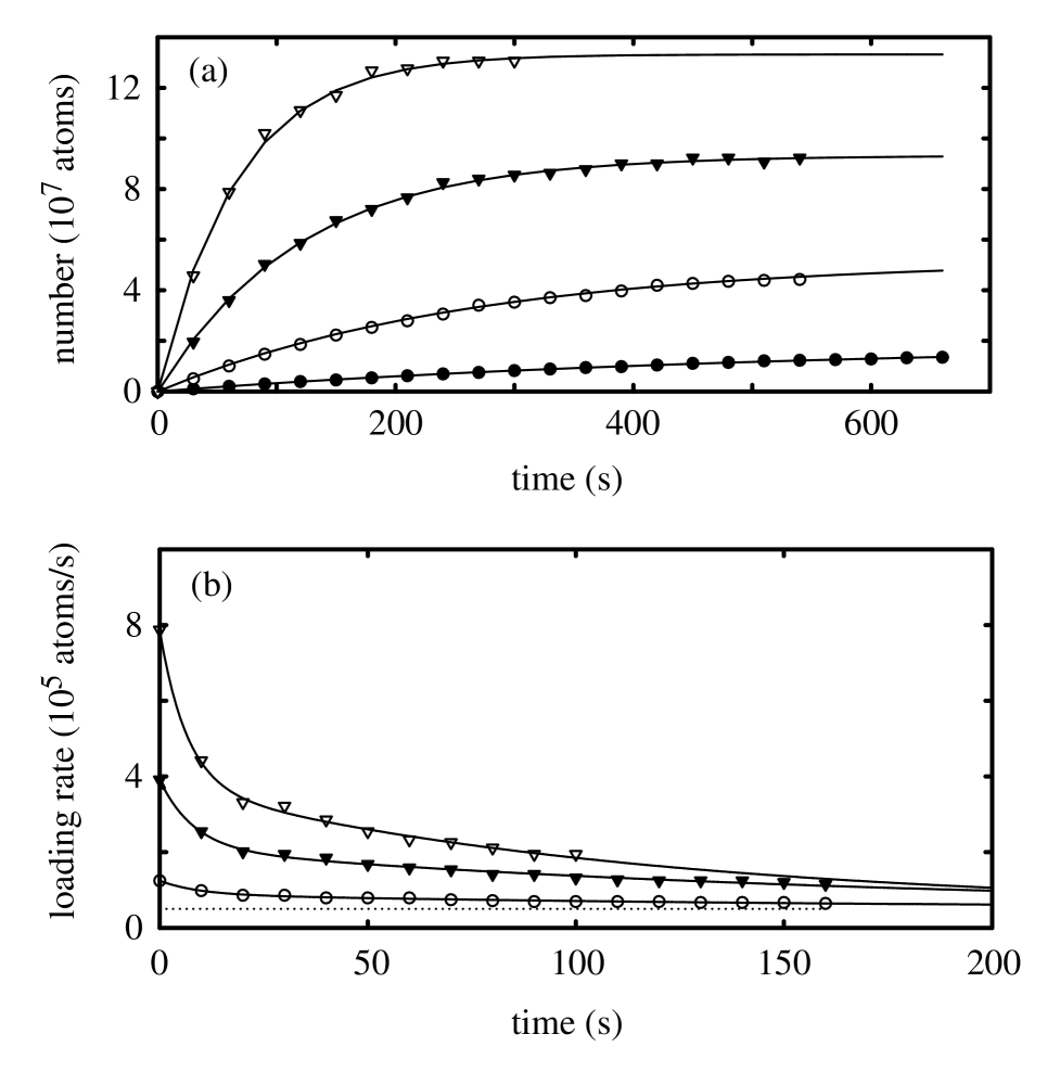
FIG. 2.: (a) Comparison of trap loading with and without the additional external white light source. (b) Trend of the loading rate as a function of time after the WLS is turned off. The lower dashed line shows the loading rate before the WLS was turned on. For both (a) and (b), open triangles represent a WLS intensity of $\sim 10$ W/cm², closed triangles represent a WLS intensity of $\sim 5$ W/cm², and the open circles represent a WLS intensity of $\sim 2$ W/cm². The closed circles in (a) represent loading without the WLS. See Table I for a numerical summary of the data shown in these plots.

A key factor to consider in optimizing $N\tau$ using the WLS scheme is the time for the vapor pressure to return to lower equilibrium values once the WLS is switched off. We define this time as the vapor pressure recovery time. A liquid nitrogen cold finger in the main chamber was used to decrease the Rb vapor pressure and shorten the recovery time after the WLS was switched off. In our cell, the cold finger had little effect on the background gas pressure, but shortened the recovery time by a factor of $\sim 2$. Furthermore, our experimental timing sequence consisted of a MOT loading phase with the WLS switched on, followed by a MOT holding phase, during which the atoms were held in a MOT with the WLS switched off. This enabled us to keep a large number of atoms trapped while waiting for the vapor pressure to decrease before extinguishing the trapping light.

In order to evaluate vapor pressure recovery times, we measured the dependence of loading rates on time just after the WLS was switched off. For the data shown in Fig. 2(b), the WLS was left on until the Rb partial pressure reached a saturated level. The WLS light was then turned off, and the number of atoms loaded into a MOT in 5 seconds was repeatedly measured. After each measurement, the MOT light was kept off for 5 s, and then the MOT started filling again for the subsequent 5 s filling rate measurement. This set of measurements indicated the speed at which $\tau_{\mbox{{MOT}}}$ and the Rb vapor pressure could recover after the WLS was turned off, and demonstrated that the recovery time was roughly independent of the WLS intensity. The fastest loading rate shown with the WLS on was $\sim 8\times 10^{5}$ atoms/s, and with the light off was $\sim 2.7\times 10^{4}$ atoms/s. Each loading rate vs. time curve in Fig. 2(b) was fit with a sum of two decaying exponential curves. The time constants for the loading rate to return to lower equilibrium values were $\sim 8$ s for the fast recovery time ($\tau_{rec,1}$), and between 113 s and 167 s for the slower recovery time ($\tau_{rec,2}$). Table I contains a list of recovery times.

TABLE I.: Loading and recovery characteristics of the MOT for various WLS strengths. $N_{\mbox{{max}}}$ indicates the maximum number of atoms that can be loaded into the trap for the corresponding Rb partial pressure. The MOT loading time constant is given by $\tau_{\mbox{{MOT}}}$ and the fast recovery time constant is listed as $\tau_{rec,1}$. The time $\tau_{rec,2}$ is the longer time constant in the exponential fits to the data shown in Fig. 2(b).

To help evaluate the vapor cell performance, the values for $N_{\mbox{{lim}}}$ and $\tau_{\mbox{{b}}}$ were estimated by measuring $N$ and $\tau_{\mbox{{MOT}}}$ for various Rb partial pressures. Experimentally, we varied the Rb partial pressure by adjusting the intensity of the WLS. We estimated $\tau_{\mbox{{b}}}\sim 700$ s and $N_{\mbox{{lim}}}=1.9\times 10^{8}$ atoms for our operating parameters by linear extrapolation with our data.

IV Model

We now describe a detailed model for determining the numbers and lifetimes of traps loaded with the WLS to demonstrate the possibility of increasing $N\tau$ under realistic experimental conditions. Specifically, this model includes the effects of finite vapor pressure recovery times and finite loading times. Without the use of the WLS, and with long loading times, $N\tau$ in a magnetic trap can obtain a maximum optimal value of

$$(N\tau)_{\mbox{{opt}}}\equiv N_{\mbox{{lim}}}\tau_{\mbox{{b}}}/4\alpha$$ (7)

with $\tau_{\mbox{{Rb}}}=\tau_{\mbox{{b}}}$. We will compare the performance of a WLS-loaded MOT to $(N\tau)_{\mbox{{opt}}}$ to demonstrate the effectiveness of a WLS-loaded MOT.

For a trap loaded with the WLS, calculating $N\tau$ is more complicated. We divide the experimental cycle into three time periods. During the first period, the MOT is loaded, and the WLS remains on for the duration of this period. We call this period the MOT loading phase, which has a duration of time $t_{1}$. The cycle then enters the MOT holding phase, which has a duration of time $t_{2}$. In the holding phase, the WLS remains off, allowing the vapor pressure to recover while continuing to hold a large fraction of the trapped atoms in the MOT. In the third period of the cycle, the MOT beams are also turned off and the atoms are trapped in a magnetic trap. This period begins at time $t_{\mbox{{T}}}=t_{1}+t_{2}$.

Variables for the number of atoms in the trap can be defined at the boundaries of the time periods. At the beginning of the loading phase, $N=0$. By the end of the loading phase at time $t_{1}$, $N_{1}$ atoms are in the MOT. The cycle then enters the holding phase, during which some atoms are lost from the trap due to collisions with other trapped atoms at a rate that is faster than the decreasing loading rate into the trap. We define $N_{\mbox{{WLS}}}$ to be the number of trapped atoms remaining at the end of this period. The “WLS” subscript emphasizes that this number was obtained using the WLS. The cycle then enters the magnetic trap phase, and $N_{\mbox{{WLS}}}$ atoms are loaded into the magnetic trap. Because of the continually decreasing vapor pressure (from having used the WLS and then turning it off), the number of atoms in the magnetic trap decays faster than exponentially. Since we desire to maximize the number-lifetime product for the magnetic trap, we define an effective lifetime $\tau_{\mbox{{WLS}}}$ as the time at which the number of atoms in the magnetic trap has reached $(1/e)N_{\mbox{{WLS}}}$. The entire cycle as described is illustrated in Fig. 3.

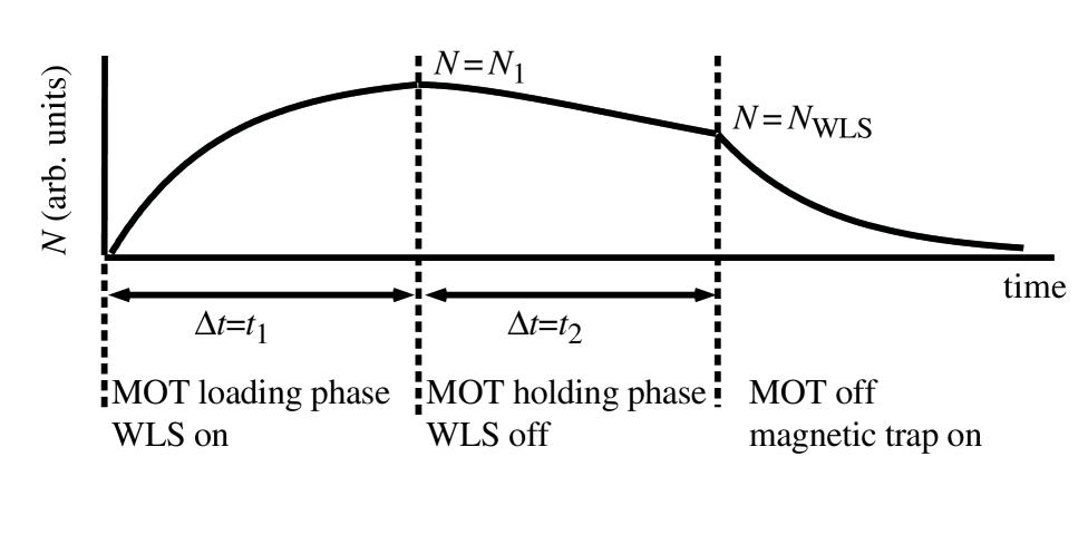
FIG. 3.: The timing sequence used in the experiment and in the calculations. The plot is a representation of the number of trapped atoms as a function of time. The dashed lines separate the different stages of trap loading and holding. The number of trapped atoms at the end of the MOT loading and holding phases is given above the $N$ vs. time curve. The states of the MOT and the WLS are also listed for the time intervals $t_{1}$ and $t_{2}$. After the MOT holding phase, at time $t_{\mbox{{T}}}=t_{1}+t_{2}$, $N_{\mbox{{WLS}}}$ atoms are assumed to be loaded from the MOT into a magnetic trap.

Our intent in this analysis is to compare $N_{\mbox{{WLS}}}\tau_{\mbox{{WLS}}}$ with both $N\tau$ for unmodulated Rb pressures at varying loading times and with $(N\tau)_{\mbox{{opt}}}$, as defined in Eq. 7. First, we calculate the number of atoms $N_{1}$ in the MOT at $t_{1}$. At the beginning of the MOT loading phase, the WLS is turned on, and the loading time constant associated with the Rb partial pressure quickly drops to a value of $\tau_{1}$. We thus obtain

$$N_{1}=\frac{N_{\mbox{{lim}}}}{1+\tau_{1}/\tau_{\mbox{{b}}}}\left[1-\exp{\left(-t_{1}\left[1/\tau_{1}+1/\tau_{\mbox{{b}}}\right]\right)}\right]$$ (8)

from the use of Eqs. 6 and 4.

The trapped atoms then enter the holding phase. The WLS is turned off, and the number of atoms in the MOT is governed by the rate equation $dN/dt=R(t)-N/\tau_{2}(t)-N/\tau_{\mbox{{b}}}$, where $\tau_{2}$ is the loading time constant associated with the decaying Rb vapor pressure. The time dependence of $R$ and $\tau_{2}$ is made explicit, since these values depend upon the decreasing Rb vapor pressure. The loading rate $R(t)$ and the loss rate $1/\tau_{2}(t)$ are assumed to decay exponentially (with a time constant of the vapor pressure recovery time) to the steady-state values $R(t)\rightarrow 0$ and $1/\tau_{2}\rightarrow 0$ (negligible Rb vapor pressures) as the vapor pressure recovers. The rate equation is numerically integrated to determine the number of atoms, $N_{\mbox{{WLS}}}$, left in the MOT at time $t_{\mbox{{T}}}$, the point at which the MOT is turned off.

We finally must determine the effective lifetime $\tau_{\mbox{{WLS}}}$ of the magnetic trapping phase of the cycle by numerically solving the rate equation $dN/dt=-\alpha(N/\tau_{3}(t)-N/\tau_{\mbox{{b}}})$. Here, $1/\tau_{3}(t)$ has an initial value of $1/\tau_{2}(t_{2})$ and decays exponentially in time to 0 as the vapor pressure continues to recover. Finally, we can write the number-lifetime product of the WLS-loaded MOT, designated by $(N\tau)_{\mbox{{WLS}}}$, as $(N\tau)_{\mbox{{WLS}}}=N_{\mbox{{WLS}}}\tau_{\mbox{{WLS}}}$.

V Results

We numerically investigated the performance of the MOT loaded with the WLS by comparing $(N\tau)_{\mbox{{WLS}}}$ with $N\tau$ for unmodulated pressures (Fig. 4). Figure 4(a) shows the number-lifetime product due to trapping atoms in a MOT for a time $t_{\mbox{{T}}}=\tau_{\mbox{{b}}}$ as a function of the fraction of the loading cycle that the WLS is used. We assume that $N_{\mbox{{max}}}=N_{\mbox{{lim}}}/2$ for unmodulated partial pressures, and an arbitrarily chosen value of $N_{\mbox{{max}}}=N_{\mbox{{lim}}}/(1+\tau_{1}/\tau_{\mbox{{b}}})=(0.9)N_{\mbox{{lim}}}$ (see Eq. 8), or equivalently $\tau_{1}=(0.1)\tau_{\mbox{{b}}}$, for the modulated partial pressures. Here, the chosen value of $N_{\mbox{{max}}}$ can not be set to $N_{\mbox{{lim}}}$ due to limitations in the numerical calculations. Fig. 4(b) shows the same conditions as Fig. 4(a), but here we have plotted the ratio of $(N\tau)_{\mbox{{WLS}}}$ to $N\tau$ with unmodulated pressures after a total MOT trapping time of $t_{\mbox{{T}}}$.

As suggested by Fig. 4, the optimum time to leave on the WLS is determined by the maximum point on a given curve. In the calculations, the gain in $N\tau$ after using the WLS is less than the maximum possible value of 4 due to the need to allow the vapor pressure to recover before loading the atoms into a magnetic trap. The highest values that can be achieved for $N\tau$ with and without the WLS are plotted against total loading time $t_{\mbox{{T}}}$ in Fig. 5 for the same conditions as in Fig. 4. The gain in using the WLS is again less than the ideal maximum factor of 4 for long loading times. However, for short loading times, $N\tau$ for unmodulated pressures is much lower than $(N\tau)_{\mbox{{opt}}}$ as shown by the gray curve in Fig. 5(a). Modulated vapor pressures can give substantial benefits in this regime, as shown by the larger $N\tau$ ratios in Fig. 5(b).

As a concrete example of reading the plots given here, we assume that we have a system that has a vapor pressure recovery time of $0.035\tau_{\mbox{{b}}}$. Thus we are interested in the uppermost curves in Figs. 4(a-d) and 5(a,b). If we load the vapor cell MOT without modulating the Rb partial pressure, we can achieve a value of $N\tau\sim 1$ (in units of $(N\tau)_{\mbox{{opt}}}\equiv N_{\mbox{{lim}}}\tau_{\mbox{{b}}}/4\alpha$) after loading the trap for a total time of $t_{\mbox{{T}}}=2\tau_{\mbox{{b}}}$, as shown in the lower (gray) curve of Fig. 5(a). However, if we modulate the Rb pressure with the WLS, we can triple the value of $N\tau$ for the same total MOT trapping time. To determine the proper time to remove the WLS light, Fig. 4(c) indicates beginning the MOT holding phase $0.12\tau_{\mbox{{b}}}$ before loading the magnetic trap (thus $t_{\mbox{{1}}}=1.88\tau_{\mbox{{b}}}$) for optimum trap loading.

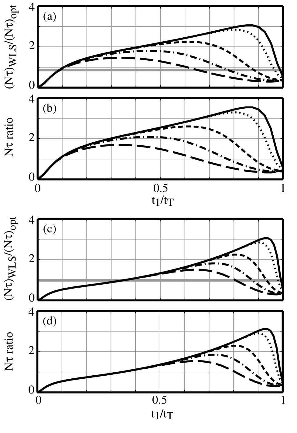
FIG. 4.: (a) The calculated products $(N\tau)_{\mbox{{WLS}}}$ in units of $(N\tau)_{\mbox{{opt}}}\equiv N_{\mbox{{lim}}}\tau_{\mbox{{b}}}/4\alpha$, the maximum value that can be achieved with unmodulated vapor pressures, after a total MOT trapping time of $t_{\mbox{{T}}}=\tau_{\mbox{{b}}}$. The Rb-limited lifetime is assumed to quickly decrease to $\tau_{1}=\tau_{\mbox{{b}}}/10$ when the WLS is turned on. The curves show $(N\tau)_{\mbox{{WLS}}}$ at varying times $t_{1}$ (as a fraction of $t_{\mbox{{T}}}$), the point in the MOT loading cycle at which the WLS is turned off, with the remaining time in the cycle ($t_{\mbox{{T}}}-t_{1}$) permitting recovery of the Rb partial pressure with a time constant of $0.035\tau_{\mbox{{b}}}$ (black line), $0.05\tau_{\mbox{{b}}}$ (dotted), $0.1\tau_{\mbox{{b}}}$ (short dashed), $0.15\tau_{\mbox{{b}}}$ (dashed-dotted), and $0.2\tau_{\mbox{{b}}}$ (long dashed). $N\tau$ for unmodulated vapor pressure is shown as a solid gray line, after a loading time of $\tau_{T}=\tau_{\mbox{{b}}}$. (Note that for this value to equal $(N\tau)_{\mbox{{opt}}}$, an infinite loading time would be needed.) (b) The ratios of the upper curves in (a) to the value of $N\tau$ for unmodulated vapor pressure after a MOT trapping time of $\tau_{T}=\tau_{\mbox{{b}}}$. (c,d) Same as for (a) and (b), with a total loading time of $t_{\mbox{{T}}}=2\tau_{\mbox{{b}}}$. Graphs (c) and (d) look nearly identical because $N\tau$ for unmodulated partial pressures is nearly equal to $(N\tau)_{\mbox{{opt}}}$ after loading for $t_{\mbox{{T}}}=2\tau_{\mbox{{b}}}$. The four graphs (a)-(d) shown in this figure demonstrate that for a given recovery time and MOT trapping time ($t_{\mbox{{T}}}$), there is an optimal WLS duration ($t_{1}$) the maximum point on the plotted curves.

Alternatively, we can shorten the loading time $t_{\mbox{{T}}}$ to $\sim 0.5\tau_{\mbox{{b}}}$, as demonstrated in Fig. 5(a), and maintain the same gain in $N\tau$. In doing so, we would not only gain a factor of 3 in $N\tau$, but we would also increase the repetition rate of the experiment by as much as a factor of 4. If instead we load the experiment for a fixed amount of time in either case (with or without the WLS), we should look at Fig. 5(b) to compare the $N\tau$ products. For a total MOT trapping time of $t_{\mbox{{T}}}=0.4\tau_{\mbox{{b}}}$, we would achieve over a five-fold gain in $N\tau$ by modulating the vapor pressure with the WLS.

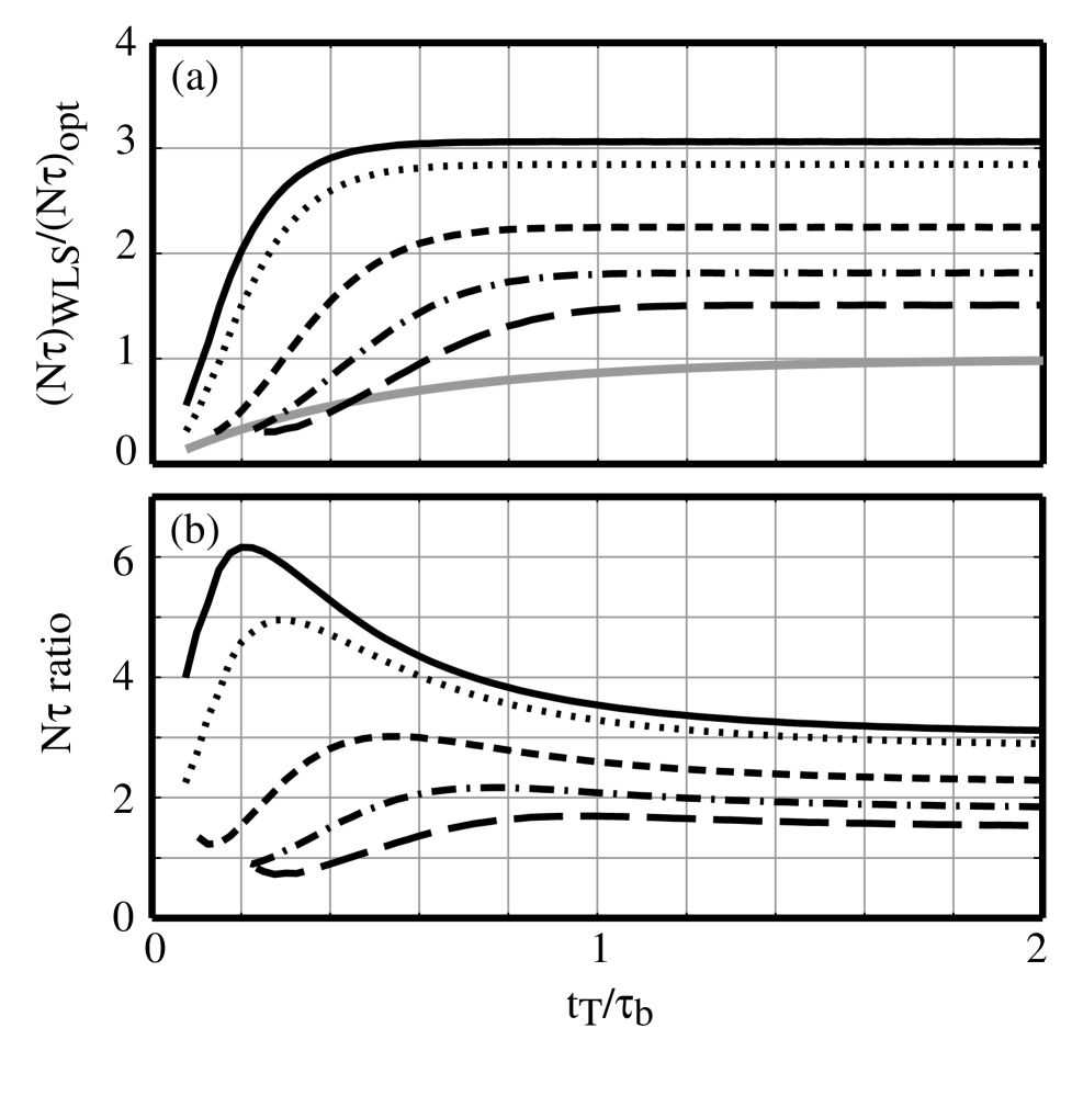
FIG. 5.: (a) Values of $(N\tau)_{\mbox{{WLS}}}$ for WLS loading as a function of $t_{\mbox{{T}}}$ (as a fraction of $\tau_{\mbox{{b}}}$). The limiting number of atoms that can possibly be loaded into the WLS trap is assumed to be $(0.9)N_{\mbox{{lim}}}$ (top curves), or equivalently $\tau_{1}=\tau_{\mbox{{b}}}/10$ when the WLS is turned on. The curves represent recovery times $0.035\tau_{\mbox{{b}}}$ (black line), $0.05\tau_{\mbox{{b}}}$ (dotted), $0.1\tau_{\mbox{{b}}}$ (short dashed), $0.15\tau_{\mbox{{b}}}$ (dashed-dotted), and $0.2\tau_{\mbox{{b}}}$ (long dashed). The variation of non-WLS number-lifetime product with time (solid gray line) is shown. The calculations assume that for any particular value of $t_{\mbox{{T}}}$, the WLS is turned off at the optimal $t_{1}$ (see Fig. 4). The vertical axis is scaled to $(N\tau)_{\mbox{{opt}}}$. (b) The ratios of the upper curves in (a) to the value of $N\tau$ for unmodulated vapor pressure at any given total MOT trapping time $t_{\mbox{{T}}}$.

Experimentally, we were able to obtain an $N\tau$ product of $(N\tau)_{\mbox{{WLS}}}=5.0\times 10^{9}$ atoms$\cdot$s using the WLS technique, achieved with a MOT loading phase of duration $t_{1}=100$ s and a MOT holding phase of duration $t_{2}$ = 50 s. This value of $(N\tau)_{\mbox{{WLS}}}$ is 2.2 times larger than $(N\tau)_{\mbox{{opt}}}=2.3\times 10^{9}$ atoms$\cdot$s, $95\%$ of the maximum value of $(N\tau)_{\mbox{{opt}}}$ for optimized Rb partial pressure, reached with a loading time of $3\tau_{\mbox{{b}}}=466$ s. Without the WLS, the Rb partial pressure was optimized when $\tau_{\mbox{{MOT}}}=\tau_{\mbox{{Rb}}}/2=\tau_{\mbox{{b}}}/2$ and $N=N_{\mbox{{lim}}}/2$. This number of $N\tau$ is inferred from measurements of $N_{\mbox{{lim}}}$ and $\tau_{\mbox{{b}}}$ mentioned previously.

Note that in addition to the gain in $N\tau$, the time to reach the above value of $(N\tau)_{\mbox{{WLS}}}$ is 3.1 times faster than the time to reach the above value of $(N\tau)_{\mbox{{opt}}}$ (without the WLS), tripling the repetition rate of experiments. The WLS experimental technique would be even more beneficial by shortening the recovery time of the vapor pressure. This might be accomplished by keeping a larger fraction of the inner surface of the vapor cell at cryogenic temperatures or through optimization of the surface adsorption chemistry.

VI Conclusions and summary

The use of LIAD to enhance loading of vapor cell MOTs may be applicable to other atomic species. Lithium vapor cells, for instance, are difficult to work with due to the high temperatures needed to create a substantial Li vapor. Yet if LIAD were to work well with Li adsorbed on stainless steel, or between co-adsorbed Li atoms on a surface, a Li vapor cell MOT would be practical. Although the effect has not yet been quantitatively explored as it has been for Rb, we observed a LIAD induced increase in the loading rate into a Cs MOT in a Cs vapor cell with aluminum walls. In general, when first using the LIAD technique, the WLS intensity should be raised incrementally to monitor the loading time constant. When the WLS loading time constant becomes too short ($<10$ s) the vapor pressure can potentially become high enough that atoms may re-adsorb onto cold chamber windows and may possibly form small clusters of atoms.

In summary, we have demonstrated that the technique of non-thermal light induced atom desorption can be used to effectively increase the number of atoms that can be loaded into a vapor cell MOT. This technique benefits atom trapping experiments where large numbers of atoms and long trap lifetimes are crucial.

REFERENCES

- [1] Current address: JILA, Campus Box 440, University of Colorado, Boulder, CO, 80309-0440.
- [2] M.H. Anderson, J.R. Ensher, M.R. Matthews, C.E. Wieman, E.A. Cornell, Science 269, 198 (1995).
- [3] K.B. Davis, M.-O. Mewes, M.R. Andrews, N.J. van Druten, D.S. Durfee, D.M. Kurn, W. Ketterle, Phys. Rev. Lett. 75, 3969 (1995).
- [4] C.C. Bradley, C.A. Sackett, J.J. Tollett, R.G. Hulet, Phys. Rev. Lett. 75, 1687 (1995); C.C. Bradley, C.A. Sackett, R.G. Hulet, Phys. Rev. Lett. 78, 985 (1997).
- [5] D.G. Fried, T.C. Killian, L. Willmann, D. Landhuis, S.C. Moss, D. Kleppner, T.J. Greytak, Phys. Rev. Lett. 81, 3811 (1998).
- [6] C. Monroe, W. Swann, H. Robinson, C. Wieman, Phys. Rev. Lett. 65, 1571 (1990).
- [7] E.L. Raab, M. Prentiss, A. Cable, S. Chu, D.E. Pritchard, Phys. Rev. Lett. 59, 2631 (1987); also see J. Opt. Soc. Am. B 6, No. 11 (1989).
- [8] C.J. Myatt, N.R. Newbury, R.W. Ghrist, S. Loutzenheiser, C.E. Wieman, Opt. Lett. 21, 290 (1996).
- [9] B.P. Anderson and M.A. Kasevich, Phys. Rev. A 59, R938 (1999).
- [10] A.M. Bonch-Bruevich, T.A. Vartanyan, Yu.M. Maksimov, S.G. Przhibel’skiĭ, V.V. Khromov, Sov. Phys. JETP 70, 993 (1990).
- [11] M. Meucci, E. Mariotti, P. Bicchi, C. Marinelli, L. Moi, Europhys. Lett. 25, 639 (1994). See also J. Xu, M. Allegrini, S. Gozzini, E. Mariotti, L. Moi, Opt. Comm. 63, 43 (1987); and E. Mariotti, S. Atutov, M. Meucci, P. Bicchi, C. Marinelli, L. Moi, Chem. Phys. 187, 111 (1994).
- [12] For a general discussion of adsorption and desorption, see Morrison, S. Roy, The Chemical Physics of Surfaces, second edition (Plenum Press) 1990; and R. Masel, Principles of Adsorption and Reaction on Solid Surfaces (John Wiley & Sons, Inc.) 1996.
- [13] T.G. Walker and P. Feng, Advances in Atomic, Molecular, and Optical Physics 34, 125 (1994).
- [14] M.H. Anderson, W. Petrich, J.R. Ensher, E.A. Cornell, Phys. Rev. A 50, R3597 (1994).
- [15] W. Ketterle, K.B. Davis, M.A. Joffe, A. Martin, D.E. Pritchard, Phys. Rev. Lett. 70, 2253 (1993).