Fixed energy inversion of 5 eV e-Xe atom scattering

Abstract

Fixed energy inverse scattering theory has been used to define central and spin-orbit Schrödinger potentials for the scattering of 5 eV polarized electrons from Xe atoms. The results are typical for a range of such data; including energies above threshold when the potentials become complex. The phase shifts obtained from an analysis of the measured differential cross section and analyzing power has been used as input data. Both semi-classical (WKB) and fully quantal inversion methods have been used to extract central and spin-orbit interactions. The analysis shows that information additional to the set of input phase shifts extracted from this (and similar) data may be needed to ascertain physical potentials.

I Introduction

A knowledge of the interaction between colliding quantum systems is central in many applications of scattering and has relevance for use in other diverse fields of study. Such interactions have been sought in various ways with the method of numerical inversion common. In the numerical inversion approach, the parameter values of a purely phenomenological parametric form, chosen a priori to be the (central, local) interaction between the colliding entities, are determined by variation until a best fit to measured data is found. Global inverse scattering methods [1] form an alternative procedural class with which to analyze the same data. With global inverse scattering methods, the interaction between the colliding pair is extracted from the data without a priori assumptions about the shape of the potential, although it may belong to a certain broad class, and the validity of the dynamical equation of motion (the Schrödinger equation) is assumed. Potentials so obtained we define hereafter as inversion potentials. Application of various global inverse scattering methods have been made in the past for electron-atom [2], for atom-atom [3], and for electron-molecule [4] systems, but none of those methods permitted extraction of spin-orbit effects. Recent developments [5, 6, 7] have provided means by which spin effects can be treated. In this paper we present and describe results for central and spin-orbit potentials obtained by global inverse scattering methods. In particular we consider an approach based upon the WKB approximation method [1, 8] and one based upon the Newton-Sabatier (N-S) theory [1].

The data of interest come from the very high quality crossed beams experiment of Gibson et al. [9]. In that study [9], a phase shift analysis was also made and the phase shifts so obtained were the input quantities to our studies. Those phase shifts are purely real in line with the unitarity constraint with the energy below the first threshold. Thus we have obtained purely real inversion potentials. Extension of the approach to deal with energies above threshold and, concomitantly with complex potentials, is straightforward. The key feature about inversion potentials, given numerical accuracy in calculations and stability of the solution, is that when used in Schrödinger equations they lead to the same phase shifts as are input.

The data set we have chosen to use is intriguing for a number of reasons. First, the differences between the values of $\delta^{+}_{l}$ and $\delta^{-}_{l}$ (the $\pm$ superscripts denoting $j=l\pm\frac{1}{2}$) extracted by the phase shift analysis [9] are not large indicating that the spin-orbit interaction is not strong. As a result the approximation method of Leeb, Huber and Fiedeldey [5] (LHF hereafter) can be used with confidence. Indeed the LHF scheme is accurate through second order in Born approximation and has worked well in some nuclear scattering data analyses [10] where the spin-orbit effect is much stronger than in the case we study. With the LHF approximation, both the N-S and the semi-classical WKB methods of inverse scattering theory can be used to specify the electron-Xenon (e-Xe) potentials. Exact quantal inversion methods to get the spin-orbit interaction are known [6, 7], but with this data the LHF approximation should be adequate and the inversion process is facilitated by its use. Second, the phase shifts of significance are not many in number and so this may be another case with which phase shift values at unphysical rational values of angular momentum are required in the inversion process to achieve a stable result [11]. A third reason for interest is that the $s$- and $p$-wave phase shifts from the analysis [9] of the scattering data have negative values. All other (physical) phase shifts of significance are positive quantities. As phase shifts are ambiguous to modulo $\pi$, an equivalent completely positive valued and monotonically decreasing phase shift set can be formed by the addition of $2\pi$ and $\pi$ to the $s$- and $p$-wave values respectively. With either of the original or the modulated (integer $l$) phase shift sets as input, the N-S inversion method per se gives the same inversion potential. However, that potential has a short ranged repulsion; such being required [12] to give significant negative $s$- and $p$-wave phase shifts. The WKB inversion method on the other hand, does discriminate between these sets since to specify the WKB inversion potential interpolated functions, $\delta_{l}(\lambda)$, are required as input. Of course if the N-S method is extended to use phase shifts at rational values of the angular momentum, found for example by interpolation of the original sets [9] and of the those with $s$- and $p$-wave values adjusted by $2\pi$ and $\pi$ respectively, then the inversion potentials from the two cases must differ.

Thus we give two new elements in this paper. First we deduce by inverse scattering theories, central and spin-orbit potentials for 5 eV electron-Xenon atom scattering. Second, we show that information additional to the physical phase shifts (i.e. those determined by usual phase shift analyses of scattering data) is needed to identify the the most likely physical inversion potential. In the next section we give a pr$\acute{\rm e}$cis of the LHF approximation for phase shifts as well as of the inverse scattering methods used, the N-S and the WKB semi-classical schemes specifically. Then in Sec. III, we discuss the origins and characteristics of the 5 eV e-Xe scattering phase shifts that have been used as input to our inversion studies. The e-Xe potentials that result are presented and discussed in Sec. IV and we draw conclusions in Sec. V.

II Fixed energy inversion methods

In this section we give brief outlines of the methods used in the calculations, the results of which we report later. First we set out the LHF scheme by which the spin-orbit interaction can be defined from two independent (spin-less) inversion calculations. This identifies not only the special phase shift sets $\{\hat{\delta}_{l}\}$ and $\{\tilde{\delta}_{l}\}$ of the method, but also defines the central and spin-orbit potentials in terms of the results of inversions of those new phase shift sets, $\hat{V}$ and $\tilde{V}$ respectively. Then we give the salient features of the Newton-Sabatier and the semi-classical WKB inverse scattering theories which we have used to specify the ($\hat{V}$ and $\tilde{V}$) potentials.

A The LHF approximation

While exact quantal inverse scattering theories that yield central and spin-orbit interactions from input scattering phase shift sets exist [6, 7], Leeb, Huber, and Fiedeldey [5] developed an approximation scheme to transform the input phase shift sets so that more facile quantal inverse scattering methods, such as the N-S scheme [1] and the semi-classical WKB approximation [8], can be used to give results from which central and spin-orbit potentials can be extracted. Those more facile schemes do not allow for an angular momentum dependence in the intrinsic equation of motion, such as given by a spin-orbit potential. They are designed only to provide central local potential functions.

The LHF method is based on the assumption that the contribution of the spin-orbit potential to the phase shifts can be evaluated using a Distorted Wave Born Approximation. This technique has been formulated specifically for spin $\frac{1}{2}$ particles incident on spin zero targets and is accurate to second order in the Born expansion [5]. The approximation identifies first the special phase shift sets $\{\hat{\delta}_{l}\}$ and $\{\tilde{\delta}_{l}\}$, and then defines the central and spin-orbit potentials in terms of the results, $\hat{V}$ and $\tilde{V}$ respectively, from inversion of those new phase shift sets.

For spin $\frac{1}{2}$ particles incident on a spin $0$ target, and allowing central and spin-orbit Schrödinger potentials, the scattering is defined by reduced radial Schrödinger equations

$$\frac{d^{2}}{d\rho^{2}}-\frac{l(l+1)}{\rho^{2}}+1-\frac{1}{E}\left[V_{cen}(\rho)+a^{\pm}_{l}V_{so}(\rho)\right]\psi^{\pm}_{l}(\rho)=0\ ,$$ (1)

where, with $\rho=kr$,

$$a^{\pm}_{l}=\frac{1}{\hbar^{2}}<{\mathbf{s}\cdot l}>\ =\left\{\begin{array}[]{cl}l&\ \ j=l+\frac{1}{2}\\ -(l+1)&\ \ j=l-\frac{1}{2}\end{array}\right.\$$ (2)

If the spin-orbit term is relatively weak, the usual scattering phase shifts, $\delta^{\pm}_{l}$, can be expanded in powers of $a^{\pm}_{l}$. Specifically [5]

$$\delta^{\pm}_{l}=\delta^{cen}_{l}+a^{\pm}_{l}C^{(1)}_{l}(k)+(a^{\pm}_{l})^{2}C^{(2)}_{l}(k)+\dots.$$ (3)

While the leading term, $\delta^{cen}_{l}$, is due solely to the central component of the potential, $V_{cen}$, higher terms must be considered to define the spin-orbit properties. But the specific analytic forms of the coefficients, $C^{(n)}_{l}$, do not have to be known to extract the central and spin-orbit potential values. The LHF approximation is initiated by considering combinations of $\delta^{+}$ and $\delta^{-}$ from which separate inversion potentials can be estimated. The relevant combinations are

$$\tilde{\delta}_{l}=\frac{1}{2l+1}\left\{(l+1)\delta^{+}_{l}+l\delta^{-}_{l}\right\}=\delta^{cen}_{l}+l(l+1)C^{(2)}_{l}+\dots,$$ (4)

and

$$\hat{\delta}_{l}=\frac{1}{2l+1}\left\{l\delta^{+}_{l}+(l+1)\delta^{-}_{l}\right\}=\delta^{cen}_{l}-C^{(1)}_{l}+(l^{2}+l+1)C^{(2)}_{l}+\dots$$ (5)

To first order in $a^{\pm}_{l}$, these new phase shifts and their inversion potentials, $\tilde{V}$ and $\hat{V}$, are

$$\tilde{\delta}_{l}=\delta^{cen}_{l} \ \leftrightarrow\ \tilde{V}\sim V_{cen}$$ (6)

$$\hat{\delta}_{l}=\delta^{cen}_{l}-C^{(1)}_{l} \ \leftrightarrow\ \hat{V}\sim V_{cen}-{1\over 2}V_{so}\ .$$ (7)

As these new sets of phase shifts can be inverted independently using any of the conventional techniques, the central and spin-orbit components can be identified then by

$$V_{cen}(r) \approx \tilde{V}(r)$$ (8)

$$V_{so}(r) \approx 2[\tilde{V}(r)-\hat{V}(r)]\ .$$ (9)

B The N-S method

Since the Newton-Sabatier inverse scattering theory and applications have been widely reported, only pertinent points of the scheme are presented herein. A full treatment on the development of this method is given elsewhere [1].

The N-S method is one of the most successful of the fixed energy inversion methods. Very recently, it has been applied successfully to electron-helium atom scattering [13] using as input, experimental phase shifts of Nesbet [14] at low $\ell$-values and dipole polarization phase shifts at the higher $\ell$-values. But it is known [15] that fixed energy inverse scattering theory requires the $S$ matrix (equivalently the phase shifts) as a function of the angular momentum variable if one is to define uniquely the scattering potential. This equates to knowing the $S$ matrix exactly at all of the (infinite) set of physical $l$-values as then the unit step in the quantum number is infinitesimal against the range. Most studies of the fixed energy inverse scattering problem, and notably those involving the N-S method, have been applied using only the values of the $S$ matrix specified at a finite set ($l_{max}$) of physical angular momentum values. In cases where there are relatively few important partial wave phase shift values to be used, it may be necessary to extend [11] the usual N-S formulation to include rational values of angular momenta to form the matrix inherent in the N-S scheme [1].

However it serves to consider for this section, just the integer values of angular momentum for which the Schrödinger equations take the form ($\rho=kr$ being dimensionless)

$$D^{u}(\rho)\ \phi^{u}_{l}(\rho)=l(l+1)\ \phi^{u}_{l}(\rho)$$ (10)

where the operator

$$D^{u}(\rho)={\rho^{2}}\left[{d^{2}\over{d\rho^{2}}}+1-U(\rho)\right]$$ (11)

with $U(\rho)=V(\rho)/E_{cm}$, where $E_{cm}=\left(\hbar k\right)^{2}/\left(2\mu\right)$ and $\rho=kr$. The solutions are subject to boundary conditions

$$\phi_{l}^{u}(\rho)\mathop{\longrightarrow}_{\rho\to\infty}A_{l}\ \sin\left(\rho-\frac{1}{2}l\pi+\gamma_{l}\right)$$ (12)

with $\gamma_{l}$ being the relevant phase shifts to be taken as input quantities. The N-S method gives as output

$$U(\rho)=U_{0}(\rho)-{2\over\rho}{d\over{d\rho}}{1\over\rho}K(\rho,\rho)$$ (13)

wherein $U_{0}$ is a reference potential and $K(\rho,\rho)$ is the Jost transformation kernel which can be written as the infinite sum of solution function products,

$$K(\rho,{\rho^{\prime}})=\sum_{l}c_{l}\ \phi^{u}_{l}(\rho)\ \phi_{l}^{u_{0}}({\rho^{\prime}})$$ (14)

The solution functions (to $D^{u}$ ) can be expressed by the Newton equations [1]

$$\phi^{u}_{l}(\rho)=\phi^{u_{0}}_{l}(\rho)-\sum_{l^{\prime}}c_{l^{\prime}}\ L_{ll^{\prime}}(\rho)\ \phi^{u}_{l^{\prime}}(\rho)$$ (15)

where

$$L_{ll^{\prime}}(\rho)=\int_{0}^{\rho}\phi^{u_{0}}_{l}(\rho^{\prime})\phi^{u_{0}}_{l^{\prime}}({\rho^{\prime}}){1\over{\rho^{\prime}}^{2}}d{\rho^{\prime}}$$ (16)

These equations are of central importance. From them one can determine the unknown quantities, $A_{l}$ and $(c_{l}A_{l})$, by matching asymptotically to the defined boundary condition solutions for $\rho\geq\rho_{0}$, $\rho_{0}$ being the value at which the unknown quantal interactions are presumed to be vanishingly small. There is also a presumption that the solution functions of the reference potential are completely known so that the initiating L-matrices can be defined exactly. The reference solutions are obtained from

$$D^{u_{0}}(\rho)\ \phi^{u_{0}}_{l}(\rho)=l(l+1)\ \phi^{u_{0}}_{l}(\rho)$$ (17)

with

$$\phi^{u_{0}}_{l}(\rho)\mathop{\rightarrow}_{\rho\to\infty}\sin\left(\rho-\frac{1}{2}l\pi+\delta^{0}_{l}\right)$$ (18)

where $\delta^{0}_{l}$ is a reference input phase shift. With the normalization and expansion coefficients so given, the complete solution functions can be determined from Eq. (15) at all $\rho<\rho_{0}$. Thereby one gets the Jost transformation kernels and thence the sought after potential.

C The WKB method

In the WKB approximation with $\lambda=l+\frac{1}{2}$, scattering phase shifts are defined [1, 12] by

$$\delta(\lambda)={\pi\over 2}\lambda-kr_{0}+\int^{\infty}_{r_{0}}\left[K_{\lambda}(r^{\prime})-k\right]\ dr^{\prime}$$ (19)

where $K_{\lambda}(r)$ describes the local momentum through the interaction region and $r_{0}$ is the classical turning point. Thus the scattering potential is embedded in $K_{\lambda}(r^{\prime})$ and inversion amounts to an integral transformation. To effect such a transformation it is convenient to consider the deflection function

$$\Theta(\lambda)=2\frac{d\delta(\lambda)}{d\lambda}\ ,$$ (20)

where now $\lambda$ is taken as the angular momentum variable. This deflection function satisfies an Abel-like equation, found by applying the Sabatier transformation,

$$\sigma=kr\left[1-\frac{V_{WKB}(r)}{E}\right]^{\frac{1}{2}}$$ (21)

to Eq. (19). One finds

$$\delta(\lambda)=-\frac{1}{2E}\int^{\infty}_{\lambda}\frac{Q(\sigma)}{\sqrt{\sigma^{2}-\lambda^{2}}}\sigma d\sigma\ ,$$ (22)

where $Q(\sigma)$ is a quasi-potential defined by

$$Q(\sigma)=2E\ln\left(\frac{\sigma}{kr}\right)\ .$$ (23)

The Abel-like integral equation for $\delta(\lambda)$ can be inverted to give

$$Q(\sigma)=\frac{4E}{\pi}\frac{1}{\sigma}\frac{d}{d\sigma}\int^{\infty}_{\sigma}\frac{\delta(\lambda)}{\sqrt{\sigma^{2}-\lambda^{2}}}\lambda d\lambda\ ,$$ (24)

which can be written in terms of the deflection function as

$$Q(\sigma)=\frac{2E}{\pi}\int^{\infty}_{\sigma}\frac{\Theta(\lambda)}{{\sqrt{\sigma^{2}-\lambda^{2}}}}d\lambda\ .$$ (25)

Provided there is a one to one mapping of the transcendental equation

$$kr=\sigma\exp{\left(\frac{Q(\sigma)}{2E}\right)}\ ,$$ (26)

and the energy $E$ exceeds that at which ‘orbiting’ occurs, i.e.

$$E>V(r)+\frac{1}{2}r\frac{dV}{dr}\ ,$$ (27)

then the Sabatier transformation equation provides the relationship from which the scattering potential can be found, namely

$$V_{WKB}(r)=E\left\{1-\exp{\left[-\frac{Q(\sigma)}{E}\right]}\right\}\ .$$ (28)

For large $\sigma$, the quasi-potentials decrease so that with $\sigma\to kr$, $Q(\sigma)\to V(r)$. As $\sigma\to 0$ however, the quasi-potentials diverge and the transforms then lead to the lower limits $r\longrightarrow r_{0}$ (the turning point radius), $V(r)\longrightarrow E\$. However, in practical cases the validity of the WKB approximation breaks down at a radius larger than $r_{0}$, when the transcendental relationship between $\sigma$ and $r$ becomes ambiguous.

III Specification of sets of phase shifts

The 5 eV e-Xe phase shifts determined by Gibson $\it et.al.$ [9] have interesting structure notably that while the $s$- and $p$-wave phase shifts are negative, for all other $l$-values they are positive. The filled circles in Fig. 1 depict the the phase shifts that have been extracted from the data. The top most graph identifies the phase shifts associated with the $j=l+\frac{1}{2}$ angular momentum set while the bottom panel contains those associated with $j=l-\frac{1}{2}$. It is evident from the data displayed in this figure that the there is only a small difference between the $\delta^{\pm}_{l}$ sets. The largest difference occurs with the $p$-wave phase shifts, and that is only of order $0.1^{c}$.

As the phase shift analyses of the e-Xe scattering data gave negative values for the $s$- and $p$-wave phase shifts, one can expect [12] scattering potentials that have a short ranged repulsion. But for e-Xe scattering it is known that the potential should be attractive at all radii and especially so near the origin where the incoming electron should feel essentially only the presence of the nucleus. Then one would expect the phase shifts for low $l$-values to be positive. Such can be formed with the phase shift values having a monotonic decrease with $l$ by the addition of $2\pi$ to $\delta^{(+)}_{0}$ and $\pi$ to $\delta^{\pm}_{1}$. We define such modulated values as the $\pi$-adjusted phase shifts hereafter. Naturally multiples of any integer amount may be used, but this new set is the simplest. The new ($\pi$-adjusted) values are shown by the open circles in Fig. 1. Associated with such phase shifts are purely attractive interactions which are expected in the physical potentials for electron-atom scattering.

To investigate the effect of additional input on the form of the inversion potentials, the two data sets were interpolated. Several interpolations were made seeking suitable input for the different inversion schemes. A many point interpolation was made on each phase shift set to obtain the input for the WKB inversion scheme. Values of the phase shift functions had to be found at quite small step sizes, $\Delta l$, since in the WKB we have to evaluate not only the deflection functions but also integrate over them (numerically). A step size $\Delta l$ of $0.01$ was used. Also two extended sets of input phase shift values were generated for use with the N-S scheme. One had $\Delta l=0.5$ and the other $\Delta l=0.2$. This was done to assess the effect of differing numbers of non-physical input on the N-S inversion potentials. The sets of interpolated phase shifts obtained using $\Delta l=0.2$ are displayed in Fig. 1, with the solid and dashed curves giving the results of those (spline) interpolations. Clearly the phase shift functions so specified are no longer equivalent and so we expect any inversion process that requires such functions as input to give different inversion potentials.

IV Results and discussion

The results we have obtained using the N-S inverse scattering theory are discussed first and, subsequently, those found from our WKB study of the chosen two phase shift functions are considered. We present in three subsections, the potentials that result, the phase shifts found from solutions of the Schrödinger equations containing those potentials, and the cross sections that ensue in each case.

A The results from N-S inverse scattering theory

Our N-S studies have lead to six inversion potentials; three found by using the original phase shift values of Gibson et al. [9] and the other three obtained by using the $\pi$-adjusted phase shifts. For each case, we first calculated the N-S inversion potentials using as input solely the phase shifts corresponding to the physical $l$ angular momentum set $l\in{0,1,2,...,7}$. Such results we identify as case 1 results, e.g. case 1 inversion potentials from the $\pi$-adjusted phase shift sets. Two other calculations have been made with N-S inversion. First the N-S inverse scattering theory equations have been solved using the discretization $\Delta l=0.5$; the results we identify by the designation case 2. The third set of N-S calculations were made using $\Delta l=0.2$ to give what we term case 3 results.

1 The N-S inversion potentials

Physical arguments dictate that the e-Xe scattering potential for 5 eV electrons should be real (the energy is below the first threshold) and to be attractive, with long range behavior of ${-|\alpha|/r^{4}}$ and a short ranged one of ${-Ze^{2}/r}$. One may also expect that the intermediate range potential would be essentially a monotonic function between the extremes as the charge density of the atom is believed to be a smooth function

The potentials resulting from the inversion of the phase shifts based upon the original set [9] are all strongly repulsive at small radii and hence are not considered physically significant. They also have marked oscillation in both their central and spin-orbit results. When used in the Schrödinger equations however, the solutions do reproduce the input phase shifts quite well; comparable to the results we show subsequently. But as the inversion potentials are not consistent with the form of e-Xe potential dictated by knowledge of that scattering system, we consider those inversion results no further.

In Fig. 2 the potentials obtained by inversion of the $\pi$-adjusted phase shift values are displayed. The top and bottom segments portray the central and spin-orbit components of the potentials respectively. The dashed, long dashed, and solid curves represent the case 1, case 2, and case 3 potentials respectively. The dashed curves in this figure are identical to the results of inversion found using the original phase shift values of Gibson et al. [9] That is as should be since within the N-S inversion scheme made with just the phase shift values specified at the physical angular momenta, modulo $\pi$ adjustment means that one uses exactly the same expansion wave functions in defining the internal matrices. But the other cases have quite different outcomes. The potentials shown in Fig. 2 tend to the physical expectation and clearly demonstrate that the inclusion of greater numbers of phase shifts at non-integer angular momentum lead to smoother, more realistic potential forms. The inversion potential found using the phase shifts at solely the physical angular momenta does not represent a structure expected for 5 eV electrons on Xe atoms as it has the short ranged repulsion. However between 0.75 and 2.5 a.u., that (case 1 central) potential has an attractive well with a depth of -1.3 a.u. while beyond 2.5 a.u. it behaves approximately as $r^{-4}$. The spin-orbit component of the case 1 potential is very small, is weakly attractive in the vicinity of 1 a.u., mildly repulsive between 1 and 2.5 a.u., and after that it is essentially zero.

Obviously the most realistic potential comes with the case 3 potentials found using the $\pi$-adjusted phase shift sets. That concurs with the hypothesis that the inverse scattering theory result stabilizes with increase in the number of non-integer angular momenta phase shifts commensurate with numerical accuracy of evaluation. Essentially the angular momentum step size should be small in comparison to the number of significant partial wave input data ($l_{max}$). This case 3 potential, shown in Fig. 2 by the solid lines, has exactly the structure one would associate with e-Xe scattering. At small radii it is strongly attractive and of $r^{-1}$ form, with a smooth transition to a long range $r^{-4}$ tail. There is a smooth transition between those regions. The spin-orbit results also are more reasonable. The case 3 (with $\pi$-adjusted phase shifts as input), spin-orbit potential is not as extensive as the others. But the spin-orbit potentials are all small in general (save for the naturally occurring divergence at the origin) and so these three results do not by themselves indicate convergence. The reproduction of phase shifts and observables, however, tend to suggest that the results we show are reasonable.

2 Reproduction of the phase shifts

An indication of the success of an inversion scheme is to reproduce the input phase shifts from solutions of the Schrödinger equations using the inversion potentials. In this case such reproduction is reasonably good but not exact; perhaps being a measure of the LHF approximation.

In Fig. 3, the original phase shift values [9] are portrayed by the filled circles and are compared with those obtained (at integer angular momenta) using each of the three inversion potentials defined by the $\pi$-adjusted input sets. Case 1 results lie within the filled circles, case 2 values are shown by the open squares, and case 3 gave the results portrayed by the open circles. The three lines now are meant only to guide the eye by connecting the phase shift values arising from use of the three inversion potentials.

The best reproduction of the phase shifts defined from experiment [9] is found by using the case 1 inversion potential, notwithstanding that the potential contains unphysical characteristics. Essentially, the inversion scheme in this case produces a potential that has been defined from just the two sets of eight phase shift values found by Gibson et al. at the physical values of $l=0$ to $l=7$. Case 2 and 3 potentials, on the other hand, were built using many more phase shifts specified at non-integer $l$-values and as the inversion potentials then seek to reproduce all of those extra values equally well, small variations in the results at the 8 physical $l$-values from the sets of Gibson et al. can result. The choice of those additional (unphysical) phase shifts then is crucial if the resulting potentials are to reproduce the eight physical values very well. One has to balance the need for a sufficiently large basis so that the inversion potential has stabilized to the proper (physically credible) limit, against the numerical accuracy one needs to achieve with reproduction of the physical phase shifts and scattering data.

A source of possible error in addition is the choice that must be taken for the phase shift at the unphysical point $\delta^{j=-\frac{1}{2}}_{0}$. That value is needed in the calculations of both $\tilde{\delta}$ and $\hat{\delta}$ and also in the N-S scheme. This choice has the potential to introduce error since its value influences the interpolation. A poor choice of this value can become evident when the inversion potential is used to recalculate the phase shifts, particularly for the low-$l$ partial waves. A reasonable choice seems to be to set the phase shift $\delta^{j=-\frac{1}{2}}_{0}$ equal to $\delta^{j=+\frac{1}{2}}_{0}$. Admittedly this is an arbitrary point. In this study, two choices were considered; the first being to take $\delta^{j=-\frac{1}{2}}_{0}=\delta^{j=+\frac{1}{2}}_{0}$ and the other to use an Akima spline to determine the value by extrapolation. In this study allowing the Akima spline to determine this point was slightly more successful.

3 The cross section from the N-S inversion potentials

Although the potentials all look reasonably good, particularly that found from case 3 with the $\pi$-adjusted input phase shifts, the further test of the inversion results is to see how accurately use of the potentials reproduce experimental data. This is displayed in Fig. 4 wherein the experimental data (with error bars) as found by Gibson et al. [9] are compared with the cross sections calculated from the three inversion potentials obtained using the $\pi$-adjusted phase shift sets. Those results found using the case 1, case 2, and case 3 inversion potentials are depicted by the dashed, long dashed , and solid curves respectively. Further we display the results here on a linear scale to distinguish the bulk of the results in relationship to the error bars. Later when discussing the WKB calculated cross sections, we will display also the case 3 N-S comparison with data shown on a semi-logarithmic plot. That emphasizes the comparison of results with data at the large scattering angles and particularly in the vicinity of the minima as 120^∘. As one might expect from the reproduction of the phase shifts, we see in Fig. 4 that a good reproduction of the cross-section data is found with the case 1 results. That result passes through the error bars of most data points. The case 2 cross section has similar structure to the experimental data, but the shape is slightly at variance falling just outside the error bars associated with a number of the data. The case 3 cross section however is in excellent agreement with most of the experimental data. In general it falls within most of the data error bars except at the larger scattering angles; the latter indicative of the phase shifts at integer values of $l$ not being reproduced with sufficient accuracy.

B The results from semi-classical WKB inversion theory

The WKB inversion results have been obtained by forming the $\tilde{\delta}(\lambda)$ and $\hat{\delta}(\lambda)$ phase shift functions and using them to evaluate two quasi-potentials. The potentials that result are discussed in the first subsection. Subsequently we present and discuss the phase shift reproductions and the cross sections that result on using those inversion potentials.

1 The WKB inversion potentials

The inversion potentials we have found using the semi-classical WKB methods are presented in Fig. 5. Once again the central potential is shown in the top section of the figure; the spin-orbit potential in the bottom. Clearly two very different structures have been generated. The result from using the $\pi$-adjusted functions has physically sensible characteristics but that found using the deflection function defined from the original phase shifts does not. Indeed the inversion procedure based upon the original phase shift set does not lead to a spin-orbit potential one can identify as anything sensible and so that is not displayed.

The $\pi$-adjusted phase shift data sets give smooth monotonic phase shift functions and hence work well with the WKB scheme. Furthermore it leads to the form of potential (the continuous lines in Fig. 5) one would expect for the central component of an e-Xe interaction, i.e. a smooth function which is highly attractive toward the origin and has an attractive $r^{-4}$ long range behavior. The spin-orbit component of the potential would also be small and short ranged. Essentially the potential from this WKB analysis that is displayed in Fig. 5 has this desired prescription. However, given that the input was not optimally smooth at large angular momenta (close inspection of the input data showed that there were small oscillations in the phase shift functions), there are small oscillations at large radii in the WKB inversion potential. Nevertheless, by smoothing, the long range WKB inversion potential does behave on average like $r^{-4}$ and the central component of this WKB inversion potential resembles that found using the N-S scheme.

Only the central potential found from WKB inversion of the original phase shift data [9] is shown in Fig. 5 (by the long dashed line). Quite evidently it is nonsensical. It exhibits ambiguous behavior at many radii, resulting from a loss of 1:1 correspondence between $\sigma$ and $r$ in this case. Apparently if the input phase shift function contains a large degree of curvature then that input is unsuitable for use with the WKB procedure. This is emphasized when one considers the deflection function, quasi-potential, and the associated $\sigma$ vs $r$ plots. The deflection function resulting from differentiating the phase shift function defined from interpolation of the original phase shift values, has a rapid variation as is evident from the top panel in Fig. 6. Consequently the quasi-potential will also be quite structured and that is shown in the middle panel of Fig. 6. As a result the stability condition breaks down at a fairly large radius. This condition, the correspondence between $\sigma$ and $r$, is displayed in the bottom section of Fig. 6. Clearly between 3 and 5 a.u. there is an ambiguous relation with $\sigma$ and so one finds ambiguous values of the associated WKB inversion potential in that region. Indeed one can only hope to ascribe a sensible result with this input to the WKB inversion for radii then in excess of 4 - 5 a.u.

The realistic e-Xe potentials found by using the $\pi$-adjusted phase shift sets and with both the N-S (case 3) and WKB inversion schemes, are compared in Fig. 7. The potentials found using the N-S scheme are shown by the solid curves while those found by WKB inversion are displayed by the filled circles. The latter are taken to the limit radius at which the 1:1 correspondence between $\sigma$ and $r$ is maintained. Overall the (semi-classical) WKB potentials compare very well with those found using the (full quantal) N-S scheme. Clearly the central potentials look almost exactly the same. There are differences between those two which become apparent when the observables are calculated. On the other hand, the spin-orbit WKB potential is very smooth and weak in comparison to the corresponding N-S component. Also it is repulsive at all radii while the N-S potential has a small attractive well between approximately 0.3 and 0.6 a.u.

2 Reproduction of the phase shifts

Despite the very pleasing form generated for the potential using the WKB scheme, the reproduction of the phase shifts, although reasonable, is not as good as those generated using the N-S scheme. However this discrepancy is not disconcerting given that the WKB scheme is a semi-classical approximation. The phase shifts found from our WKB calculation are shown by the open circles in Fig. 8, and joining lines have been included solely to guide the eye. The data of Gibson et al. [9] again are represented by the filled black circles. As with the N-S case, part of the discrepancy between the calculated values and the data may be due to the ambiguity with the interpolation required to specify the phase shift functions and particularly for points below $l=1$ for the $j=l-\frac{1}{2}$ input set.

A spline was used to determine the deflection function, and that influences the quasi-potential and ultimately also the potential. Given that points found from the $j=l-\frac{1}{2}$ input set are extrapolated for values of $\lambda<\frac{1}{2}$, ambiguity in those values is inevitable. That ambiguity persists when these splined values are used to determine the input functions $\tilde{\delta_{l}}(\lambda)$ and $\hat{\delta_{l}}(\lambda)$. That may result in a poor reproduction of the physical phase shifts, particularly of the $s$- and $p$-wave values when the solutions of the Schrödinger equations specified with the relevant WKB potentials are found to complete the study loop.

3 The cross section from the WKB inversion potentials

Already, from the reproduction of the phase shifts, we suspect that with the WKB method, reproduction of the cross section will not be as good as that obtained using the relevant N-S inversion potentials. This is indeed true. The solid curve shown in Fig. 9 depicts the WKB cross section result which is compared therein against the Gibson et al. data [9] and also against the cross section determined by using the preferred case 3 N-S inversion potential (shown by the dashed curve). We now present the results in a semi-logarithmic plot since WKB cross section is similar in magnitude to the data, however it does not display quite the right structure at any scattering angle. The reproduction simply is not as good as that found using the N-S scheme. This figure also emphasizes the mismatch of the case 3 N-S inversion results at large angles that we commented on earlier.

V Conclusions

Inversion potentials for the 5 eV electron-Xenon atom interaction have been found using both the full quantal N-S and the semi-classical WKB inverse scattering theories. The results from application of the N-S inversion were very good. Several inputs were used in this approach, each containing a different number of phase shift values. From solutions of the Schrödinger equations specified with each of the potentials, ‘inversion’ phase shifts were extracted that reproduced well the starting (physical) phase shift values and also the empirical cross section. However, when the input was taken solely to be the (physical) phase shifts at integer-$l$ values of angular momenta, the inversion potential contains a marked repulsion at small radii. That is not physical. With increased numbers of input data specified at non-integer values of angular momentum, inversion produced a potential with sensible (physically credible) characteristics.

As two disparate inversion methods find central e-Xe potentials that are essentially the same and have pertinent physical properties of the scattering system, we are confident that the N-S approach has (nearly) converged and that the central potential obtained by expanded $\pi$-adjusted physical phase shift sets is the appropriate candidate for the local Schrödinger interaction. The spin-orbit potential is reasonable but more detailed investigations are needed before the characteristics found for it can be adopted with confidence.

The similarity between the WKB and N-S inversion potentials also implies that the introduction of unphysical phase shifts in the N-S calculation is essential if a stable inversion potential is to be obtained in this case. That would be so with other energies measured [9] and, by implication, for any such electron-atom scattering at eV energies. There is the difficulty however, of accurately specifying the phase shifts for non-integer angular momenta. Obviously some kind of a priori information regarding the colliding system is necessary. In this instance simply $\pi$-adjusting the given phase shift data sufficed.

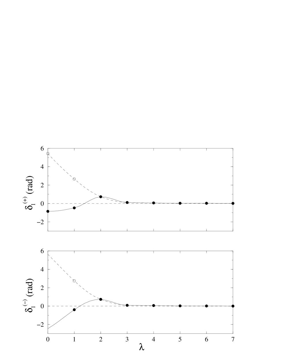
FIG. 1.: The scattering phase shifts found from a phase shift analysis of 5 eV e-Xe scattering data. The filled circles are the results specified by Gibson et al. [9] while the open circle are the $\pi$-adjusted values. The results of interpolations of the basic two sets of (physical) phase shifts are portrayed by the solid and dashed curves.

FIG. 2.: Potentials (central top; spin-orbit bottom) obtained from N-S inversion of the three sets of phase shift values described in the text and formed by using the $\pi$-adjusted phase shift values. The dashed, long dashed and solid curves depict the results designated cases 1, 2, and 3 in the text respectively.

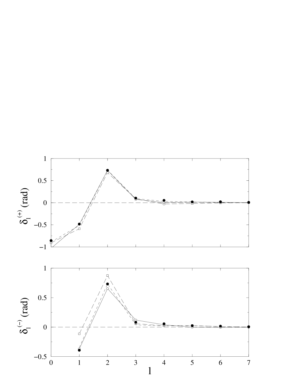
FIG. 3.: The 5 eV e-Xe phase shifts obtained from the potentials shown in Fig. 2 compared with the values specified by Gibson et al. [9]. Note that the lines are simply to guide the eye and to identify the three cases. The notation is as used in Fig. 2.

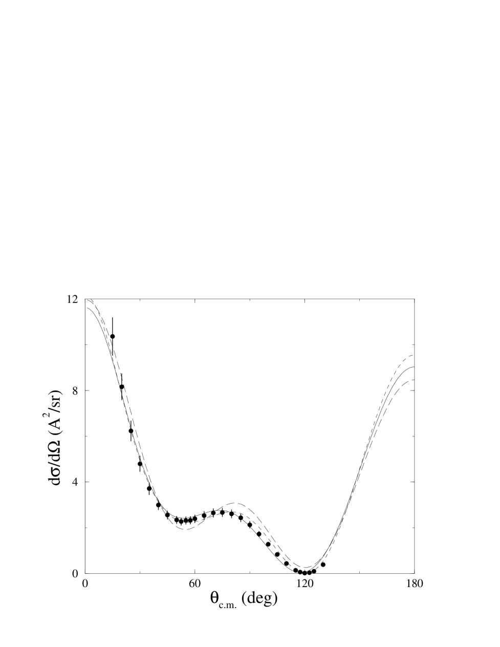
FIG. 4.: The 5 eV e-Xe differential cross sections obtained from the potentials shown in Fig. 2 compared with the data of Gibson et al. [9] (dots with error bars). The notation defining the results from the three cases is as in Fig. 2.

FIG. 5.: Potentials (central top; spin-orbit bottom) obtained from WKB inversion of the phase shift functions described in the text. The solid curves depict the results found using the $\pi$-adjusted phase shifts to define the phase shift function; the long dashed curve gives the (central) potential found using actual Gibson et al. [9] tabled values for that purpose.

FIG. 6.: The deflection function (top), the quasi-potential (middle), and the $\sigma$ vs $r$ plot (bottom) from the WKB study framed upon the original phase shift values of Gibson et al. [9].

FIG. 7.: Comparison of the WKB inversion potentials (filled circles) with those of the case 3 N-S inversion study made using phase shift sets from interpolation of the $\pi$-adjusted phase shifts of Gibson et al. [9].

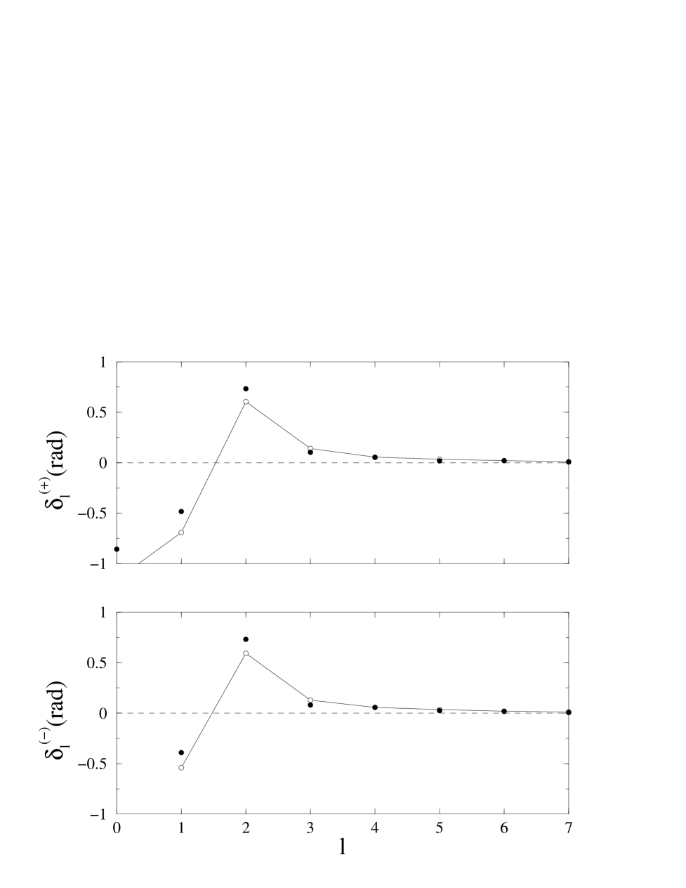
FIG. 8.: The 5 eV e-Xe phase shifts obtained from the (realistic) potential shown in Fig. 5 compared with the values specified by Gibson et al. [9]. Note that the lines are simply to guide the eye.

FIG. 9.: The 5 eV e-Xe differential cross section obtained from the WKB potential (solid curve) compared with the data of Gibson et al. [9] as well as with the case 3 N-S result (dashed curve). Both inversion studies used interpolations of the $\pi$-adjusted set of phase shifts as input data.

REFERENCES

- [1] K. Chadan and P. S. Sabatier. Inverse Problems in Quantum Scattering Theory Edition (Berlin, Springer, 1989).
- [2] L. J. Allen. Phys. Rev. A 34, 2708 (1986); L. J. Allen and I. E. McCarthy. Phys. Rev. A 36, 2570 (1987).
- [3] D. R. Lun, X. J. Chen, L. J. Allen, and K. Amos, Phys. Rev. A 50, 4025 (1994).
- [4] D. R. Lun, K. Amos, and L. J. Allen, Phys. Rev. A 53, 831 (1996).
- [5] H. Leeb, H. Huber, and H. Fiedeldey, Phys. Letts. B344, 18 (1995).
- [6] H. Huber and H. Leeb, Eur. Phys. J. A1, 221 (1998); J. Phys. G 24, 1287 (1998).
- [7] D. R. Lun and S. J. Buckman, Phys. Rev. Lett. 79, 541 (1997); D. R. Lun, M. Eberspächer, K. Amos, W. Scheid, and S. J. Buckman, Phys. Rev. A 58, 4993 (1998).
- [8] H. Fiedeldey, R. Lipperheide, K. Naidoo and S. A. Sofianos Phys. Rev. C 30, 434 (1984).
- [9] J. C. Gibson, D. R. Lun, L. J. Allen, R. P. McEachran, L. A. Parcell, and S. J. Buckman, J. Phys B 31, 3949 (1998).
- [10] N. Alexander, K. Amos, B. Apagyi, and D. R. Lun, Phys. Rev. C 53, 88 (1996).
- [11] M. Eberspächer, K. Amos, and B. Apagyi, Phys. Rev. C 61, 64605 (2000).
- [12] R. G. Newton, Scattering of Waves and Particles, 2nd edition, (Springer-Verlag, New York), (1982).
- [13] Z. Harman, Elektron-hélium ütközés effektív kölcsönhatásának meghatározása kísérleti szórásadatokból, Scientific Student Work, (Technical University of Budapest), Budapest, 1999 (unpublished).
- [14] R. K. Nesbet. J. Phys. B12, L243 (1979); Phys. Rev. A 20, 58 (1979).
- [15] J. J. Loeffel, Ann. Inst. Henri Poincare 8, 339 (1968).