A realistic quasi-physical model of the 100 metre dash
J. R. Mureika††thanks: newt@palmtree.physics.utoronto.ca
Department of Physics
University of Toronto
Toronto, Ontario Canada M5S 1A7
PACS No. : Primary 01.80; Secondary: 02.60L
Keywords: Mathematical modeling, sprinting, wind/altitude assistance, Track and Field
Abstract
A quasi-physical model (having both physical and mathematical roots)
of sprint performances is presented,
accounting for the influence of drag modification via wind and altitude
variations. The race time corrections for both men and women sprinters are discussed, and
theoretical estimates for the associated drag areas are presented.
The corrections are consistent with constant-wind estimates of previous authors, however
those for variable wind are more accentuated for this model.
As a practical example, the nullified World Record
and 1988 Olympic 100 m race of Ben Johnson is studied, and compared
with the present World Record of 9.79 s.
1 Introduction
Mathematical models of athletic sprinting/running performances, in some form or another, date back to at least the early 1900s. A. V. Hill [1] was one of the pioneers to study a sprinter’s “velocity curve”, or i.e. the runner’s speed as a function of time. Mathematician Joseph Keller [2] formulated a simplistic model to predict potential race times over a variety of distances. His method involved optimizing the set of coupled differential equations
| (1) |
with the race distance calculated as the integral
| (2) |
In Equation (1), is a decay constant which places upper limitations on maximum velocities and velocity profiles. Solutions are obtained by solving Equation 2 subject to the initial conditions , . Keller’s original model for sprint races proposed a constant propulsive force, , arguing that the athlete must use his/her entire strength to maximize their performance. In the works of Tibshirani [3] and Mureika [4], the propulsive term is adjusted to vary with time, since such intense physical exertion will inevitably introduce muscular fatigue. Explicitly, a linear decrease was chosen, , where .
2 Quasi-physical model
While Tibshirani’s model yields an approximate match of final times, it does not completely represent a simulation of an actual race. A realistic model of a sprint race should be able to accurately reproduce the critical 10 m split data which is available111A “split” is defined as the elapsed time at each 10 m division of the race, or the time-interval in which a 10 m stretch is covered. The athlete’s instantaneous velocities may be obtained for each 10 m increment, but due to technological and financial restrictions, this type of data is currently rare.. In order to better realize this approximation, the equation of motion (1) is modified as follows:
| (3) |
The term “quasi-physical” has been adopted to highlight the fact that Equation (3) is actually a mix of both mathematical and physical components. It is not a fully physical representation, nor is is a purely mathematical model, although it can be used to effectively study and estimate key physical quantities (such as the elusive drag area of sprinters).
The components of Equation (3) are defined in the following subsections.
2.1 Drive term
A sprint race can be broken into roughly three different phases: the drive, transition, and maintenance phases. Previous models of sprint performances (e.g. [2, 3, 4] and references therein) assign a singular propulsive term in the equation of motion. These do not explicitly account for the drive phase, in which a sprinter begins a race from a crouched start. From this position, the athlete is able to achieve greater speed due to increased application of forces (efficient drive posture). This phase of the race lasts for only about the first 25-30 metres, at which time the sprinter has transitioned to an upright running stance.
In the current model the following form of the drive term is adopted:
| (4) |
where is the magnitude of the drive, and a constant to be determined. The dependence ensures that the term drops off rapidly as the race progresses. In fact, after roughly seconds, the magnitude of the term drops to less than of its original value, which would correspond roughly to the appropriate distance described above.
2.2 Maintenance term
This term is left relatively intact from the previous models, but assumes a slightly different interpretation. Once the drive term has dissipated, this term is the only remaining propulsive component of Equation 3, and represents the maintenance phase of the race. Explicitly,
| (5) |
Note that, unlike the linear maintenance term assumed in [3, 4], the time-dependence assumed herein is non-negative . Certainly, this is a much more realistic assumption.
Due to the adoption of the drive term (4), the value of tends to be lower than predicted in previous models. While this does not immediately effect predictions for 100 metre performances, it does have significant implications for 200 metre dash simulations (for which previous models have made rather generous performance predictions; these are discussed in detail in a forthcoming article [5]). This difference is further discussed in Section 3.3.
2.3 Velocity term
The first of two counter-propulsive terms, the velocity term is another relic of the original Keller model, which accounts for a predicted dependence in the equation of motion. Such a term has some conceivable physical interpretations: there must exist a physical barrier which limits the maximum speed of a human, based more than just on pure muscular strength. It seems logical to assume that a sprinter’s acceleration is curtailed with increasing speed (e.g. leg-turnover or stride rate are physically and physiologically-constrained quantities). The term is written
| (6) |
with a positive constant. A reasonable assumption might be that the value of this parameter (based on the interpretation above) is a “physiological constant” for most sprinters, and should not vary significantly from a prescribed value. Most world-class sprinters show stride-rates of about 4-5 strides/second (see e.g. the analysis in [6]).
2.4 Drag term
Along with the drive term, this is the most significant adjustment to the model. Explicitly,
| (7) |
The athlete is thus modeled as a thin slab of frontal cross-sectional area , which is a sufficient approximation for the effects considered herein. A critical factor in (7) is the “modified drag area” . Here, the drag coefficient, and the sprinter’s mass (since these models are expressed in force per unit mass). The exact values of these parameters are unknown, since they can only be measured experimentally. Previous works [7, 8] have suggested that falls around m2. Additionally, these authors suggest that the drag coefficient assumed a value on the order of , but a recent suggestion by Linthorne [9] pegs the value as closer to . The data obtained from this model is consistent with this statement, and in fact indicates that may assume an even lower value (see Section 3).
The expression in (7) is designed as an initial correction to the cross-sectional area , representative of the transition from a crouched to upright position. Although the value is purely subjective, the actual magnitude of the correction does not significantly affect the results. It does, however, allow for a slightly greater acceleration over the first 10 m, and is a more realistic assumption than having a constant .
The important of an ambient wind in a sprint race is exemplified by this term, since its magnitude is a function of . Any non-zero tail-wind reduces the effective drag experience by the sprinter, allowing him/her greater acceleration, a greater top speed, and hence a faster overall time. A positive wind-speed corresponds to a tail-wind (i.e. wind in the direction of motion of the sprinter), while a negative wind-speed denotes a head-wind. The IAAF (International Amateur Athletic Federation) has adopted a limit of +2.0 ms-1 for a supporting wind, above which a race is deemed “wind-assisted” [10]. Since such times are not recognized as legal performances, they cannot be ratified as World Records.
Wind-speed has the dominant effect on drag, but an additional factor which affects this term is the atmospheric density, , where
| (8) |
Here, gm-3 is the sea-level density at 25 degrees Celsius, and is the measured elevation/altitude (in metres) (Dapena and Feltner [16] propose a second-order-in- correction to the altitude, which is not included here).
Races which are run at altitudes above m are deemed altitude-assisted, but unlike wind-assisted marks, these can be ratified as records. For example, at the 1968 Olympics in Mexico City ( m), World Records were set in both the 100 m and 200 m dashes, thanks to the considerable altitude (the density of air in Mexico City is roughly 76 of ). Pietro Mennea’s former 200 m record of 19.72 s was also set at altitude. Furthermore, the fastest-ever recorded 100 m clocking is 9.69 seconds by Obadele Thompson of Barbados, in April 1996 (at which time the official World Record was 9.85 s). This race was run in El Paso, Texas ( m) with a tail-wind of ms-1. Thompson’s previous 100 m performances were all slower than 10.00 s, which serves to demonstrate the extremal benefits of drag reduction.
3 Model parameters and simulation results
The coupled equations (3) and cannot be solved analytically, so one must resort to numerical methods. Thanks to the significant increase in modern processor speeds, the values of the parameters ; ; ; can be rapidly isolated. This was done using a fourth-fifth order Runge-Kutta integration scheme (written in C) run on a 500 MHz Pentium III processor supporting Linux 6.0. An iterative time-step of 0.001 s was chosen for the integration.
In order to determine extremal parameters for the model, key 10 m split data for several world class 100 m races are matched. Such data has been obtained at various world-class track meets, including the 1997 and 1999 World Championships in Athletics [11, 12], as well as the 1988 Olympic Games [6]. The instantaneous velocity splits obtained in [11] were measured with a laser-based device known as a LAVEG, which collects its data by sensing the reflectivity of 20 ns, 904 nm pulses directed at a (linearly) receding target. The cited reliability of the distance measurements is cm, at a sampling rate of up to 100 measurements per second [13].
After repeated numerical runs and adjustments to the parameters, the following set was obtained:
;
;
;
Also, ms-1; m. The simulation results are displayed in Table 1, and yield a raw (i.e. excluding reaction222Although they depend on the individual athlete and the conditions at the time of the race, reaction times tend to range between s. Reaction times below s are not allowed, as it is believed that it is not physiologically possible to surpass this limit.) time of 9.70 s, with a maximum velocity of ms-1 at 59.18 m. Such figures are in agreement with actual world class sprinters running sub-9.90 second races to better than , with the instantaneous velocity splits also matching to within 1 of the actual value (see e.g. the data in [11]).
Of course, each individual sprinter would most likely be described by a unique set of parameters, and such a task is not within the immediate scope of this paper. Also, due to the nature of the drag term (7), the effects of cross-winds are not considered in the current form of the model.
The drive-phase correction (4) is necessary to accurately reproduce the observed velocity profile over the first 30-40 metres. For example, the velocity profiles presented in [4] for sprinter Donovan Bailey of Canada give 9.32 ms-1 (10 m), 10.95 ms-1 (20 m), 11.67 ms-1 (30 m), and 11.99 ms-1 (40 m). These velocity figures are doubtful, in light of the profiles presented by actual split data [11]. It is unlikely that Bailey achieved a speed of 11.99 ms-1 as early as 40 m, and furthermore sustained speeds in excess of 12 ms-1 for an additional 40 m [4].
3.1 Wind assistance: determination of the drag coefficient and frontal cross-sectional area
The value of is isolated in conjunction with the measured effect of wind assistance by past authors [2, 14, 15], most of whom agree that a tail-wind of ms-1 will boost a 10 s 100 m sprint by about s. The results of an earlier study [16] cite corrections of s for a ms-1 wind, although one of the authors has since produced updated results which are more commensurate with the literature [17]. Table 1 also shows the effects of such a tail-wind on the predicted 100 m times, and accordingly predicts a boost of . Conversely, a head-wind of equal magnitude ( ms-1) will increase the time by s to 9.830 s. Clearly, the non-linear nature of the drag term implies that equal but opposite wind speeds will not provide equal boosts. It is reasonable to assume that there could be mild variations in these corrections, depending on variations in , but a full study of this effect is not the aim of this paper.
For a sprinter of mass 80 kg, the value indicates that the effective drag area is m2. Note that this is slightly less than the 0.3 m2 estimate of Linthorne [18]. For a cross-sectional area between m2, this suggests that the drag coefficient is between 0.46 and 0.57. Note that it may actually be erroneous to assume that the drag coefficient is constant, since the could potentially be frequent transitions to laminar flow occurring throughout the race. Also, the drag area may vary slightly from athlete to athlete.
It should be noted that while these simulation times are recorded to 0.001 seconds, official race times are reported to only 0.01 s, and official wind gauge readings to 0.1 ms-1. In actual fact, electronic/photo-finish timing is recorded to 0.001 s, and the following “rounding-up” algorithm is applied to the times: unless the third decimal place is 0, the hundredth position is rounded up. For example, Canadian sprinters Donovan Bailey and Bruny Surin have both recorded 100 m times of 9.84 s, but their pre-rounded times were actually 9.835 s and 9.833 s respectively [15]. A time of 9.831 s would be reported as 9.84 s, while 9.830 s would earn a 9.83 s rounding.
The reported value is measured from a gauge of height no more than 1.22 m, placed within 2 m from lane 1 on the in-field at a distance of 50 m from the finish line. The wind-speed is sampled for a duration of 10 s from the start of the race [10]. Wind speeds are measured to 0.01 ms-1, but are rounded in a similar fashion. However, Linthorne [19] has recently noted that measuring the wind speed in such a fashion gives an error of 0.7 ms-1 on the actual value. Such a discrepancy would certainly impact the validity of the reported times.
3.2 Altitude effects
Although altitude effects are secondary insofar as drag modification is concerned, their influence is not negligible. Table 2 demonstrates the modifications to the times of Table 1, subject to an increasing elevation. Non-zero wind effects are not included, but will be discussed in detail later on. The model predicts an advantage of seconds from sea level to a 2000 metre elevation. For a “Mexico City” altitude (approximately 2250 m), the correction to this 100 m time (with no wind) would be s, in rough agreement with the predictions of Linthorne [14] and Dapena [17]. It should be noted that the correction figures given in Reference [15] are considered to be overestimated, due to an inaccurate value of the drag area.
3.3 Graphical analysis of propulsive forces
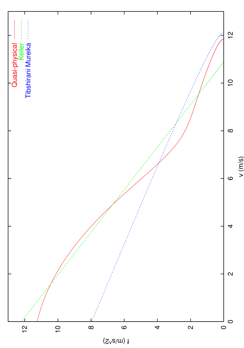
While hypothesized from a mathematical basis, the quasi-physical model herein provides accurate matches to real data. A study of the propulsive forces reveals a striking agreement to that presented by Dapena and Feltner [16]. Although their analysis is for 10.90 s-caliber sprinters, the figures presented herein for sub-10 s sprinters show the same overall structure. The authors suggest that a plot of mass-normalized propulsive force versus the athlete’s velocity can be modeled by two straight lines, adjoined at a “boundary velocity” roughly 3-5 ms-1 less than maximum.
Figure 5 demonstrates the identical analysis for the model parameters listed in Section 3. Unlike Dapena and Feltner’s model, the acceleration is highly non-linear before 4 ms-1, at which point it assumes a roughly linear form to about 7 ms-1. The “boundary velocity” in this case is representative of the point where the drive term has dropped to roughly 10 % of its original value (about 1 second into the race). At this point, the curve assumes another linear form of differing slope, before approaching the maximum velocity (and again diverging from linearity).
Such an analysis can in fact be used to rule out the Keller model and its variants. Although Keller’s value of was in the ms-2 range [2], the overall form of the function does not provide an adequate global match.
Similarly, using Tibshirani’s modification [3], the statistical fit of race data from Donovan Bailey’s 1996 Olympic 100 m race [4] predicted an initial value of 7.96 (Tibshirani’s own analysis predicted a lower value of 6.41, almost half that of Keller). These models are also presented in Figure 5, and are representative of roughly a 9.8-10 second race. On their own these two approximations do not support the predictions of the quasi-physical model, however it is interesting to note that Keller’s model before, and the Tibshirani-Mureika model after their intersection are a rough first-order approximation to the data. In fact, this is similar to linear model proposed in [16].
3.4 Assistance for women sprinters
Women sprinters are certainly lighter than an average 80 kg, yet their cross-sectional area is correspondingly smaller. Similarly, their stride rates tend to be lower. Thus, a first-pass approximation for women can be made by a mild adjustment to the parameters of Equation (3). Following the interpretation of Section 2.3, a lower stride rate can be taken to correspond to higher . Similarly, adjustments to the propulsive terms are reasonably made.
By setting , and m2 (which corresponds to a drag area of 0.18 m2 for a mass of 65 kg), one can reproduce splits which roughly replicate those observed by world class female sprinter Marion Jones (see [11]), and match the predicted wind and altitude advantages of [17] and [14]. For the cited drag area, a drag coefficient between 0.5-0.6 would require a cross-sectional area of 0.30-0.36 m2, roughly 80% that of men (a reasonable approximation).
Using these values gives a raw time of 10.653 s. At sea-level ( m), an advantage of s is predicted for a tail-wind of ms-1 (10.536 s), and s for m. These figures are again in close agreement with those of [17] and Linthorne [14], who predicts a correction of s. A wind of ms-1 at m will increase the time to 10.802 s, a difference of s.
Figures 1,2,3, and 4 give performance corrections for men and women, for altitudes ranging between m. The sign of the correction indicates the impact of the associated wind and altitude on the base time at 0 m altitude and 0-wind, i.e. . A negative correction indicates that the time is faster than the base (e.g. for tail winds), and vice versa (note the change in sign relative to the Tables). The predicted corrections for women cannot be applied to slower men’s races, since the assumed drag area is much lower. If the modified drag area is kept as 0.002875 m2kg-1, the resulting boost is s for a ms-1 wind and a lapse of s for a ms-1 wind.
4 Sensitivity to parameter variation
4.1 Correction for late-race velocity drop-off
The measured velocity data presented in Reference [11] indicate that the model predictions drop off faster than the measured data for the latter half of the race. It should be noted that this discrepancy can be accounted for by lowering the power of in maintenance term (5), and hence the overall shape of the associated “energy envelope”. In fact, the author notes that a substitution , with (and mild adjustments to ) provides a closer match to the data.
While such modifications are of interest to providing a fully realistic simulation, variation of this parameter is an over-complication of an already-intricate model, and is not essential for the study conducted herein. A full study of such time dependence is postponed for future work, and in particular its implications for the 200 m dash are discussed in [5].
Furthermore, it was noted that variation of the parameters did not significantly affect the velocity profile in the early part of the race, but could be used to adjust the late-race profile. Individual adjustments of these parameters to produce a 0.1 s advantage in the final time presented minimal effects on the profile for m. Conceivably, individual athletes could be represented by their own set of parameters, which could help account for variability in observed race times. Despite these minor velocity adjustments over 60-100 m, a ms-1 assisting wind again provided boosts between s.
4.2 Slow starts and the time dependence of
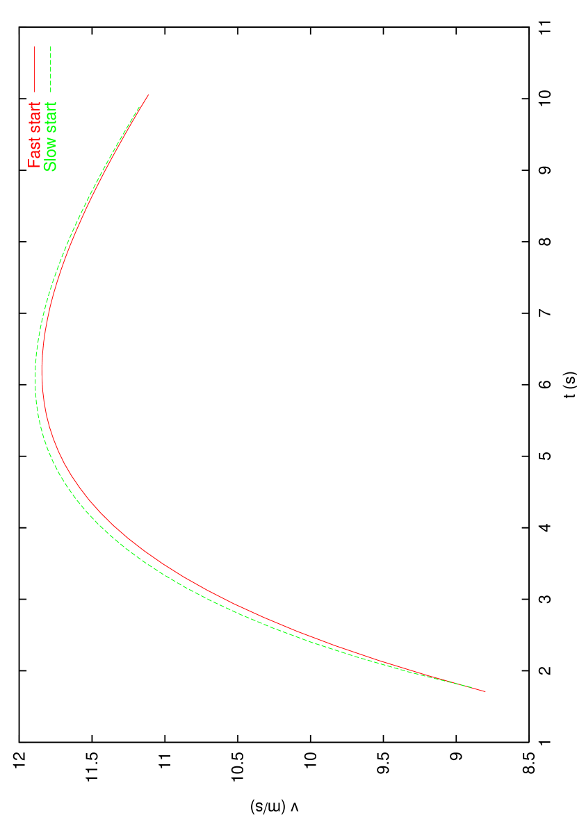
It is possible to use the model to simulate “slow starts” by suitable readjustment of the drive term parameters. In fact, by modifying the time-dependence of Equation 4, one may reproduce starts in which athletes did not accelerate as quickly as others, but achieved higher overall velocities at each split in the earlier portions of the race.
Figure 6 demonstrates such a simulation, with adjusted time-dependence , and , as compared to the simulation of Section 3. The simulated splits are shown in Table 4; such data is consistent in profile with those of Canadian sprinter Donovan Bailey from the 1997 World Championships in Athens [11]. One can note this simulation lags behind the other until about 70 metres, although achieving higher maximal velocities. In this case, the finish is within 0.005 seconds. This type of behavior is frequently observable at any competition, and is characteristic of many famous world class sprinters (including the aforementioned Bailey, as well as American track legend Carl Lewis).
5 Variable wind speeds
As mentioned previously, the wind speeds are sampled for a period of 10 seconds following the start of the race, after which the average value of the wind-speed is taken as the official gauge reading. The examples cited previously have assumed that the wind velocity is constant. However, this is probably more of ideal situation than not. A more realistic scenario is one in which the wind speed is variable, but averages out to a value which may be unrepresentative of the true conditions.
Following the example of Dapena and Feltner [16], the results of a variable-wind race are given in Table 3. Four separate variability conditions are simulated, with the constraint that the gauge reading (i.e. the mean wind velocity over 10 seconds) be the legal limit of ms-1. These conditions include:
-
1.
Step function:
-
2.
Step function:
-
3.
Linear:
-
4.
Linear:
Here, is the Heavyside function, with , and otherwise. The time-averaged wind-speed is calculated in the usual fashion, , with seconds.
While the constant tail-wind speed of ms-1 predicts a boost of 0.104 s for the present model, the above conditions predict a rather large range of variation. Cases 1 and 3 show the smallest advantages, due to minimal (or zero) wind conditions in the drive phase (hence lower overall accelerations in the first half of the race). These cases also show the lowest peak velocities in this boost scenario, although still lower than the constant wind case. Note that the peak velocities occur much later than in the base case and the constant-wind case.
Case 4 shows a peak velocity at roughly the same location as in the base 9.700 s run (a difference of only 19 cm), although with a much higher magnitude ( ms-1). Case 2, on the other hand, shows almost the same velocity, but at a much earlier mark (54.95 m). This decidedly premature maximum is no doubt due to the overpowering contributions of the velocity term once the assisting tail-wind has subsided. The sprinter is physically unable to achieve a higher velocity.
Dapena and Feltner only consider Cases 1 and 2 in their analysis (for the time-averaged +2 ms-1 wind). However, it is interesting that the predictions of this model in fact are opposite of their assertions. For Case 1, they predict a boost of 0.066 s, while their Case 2 shows a boost of 0.060 s, both lower than their constant-wind case (0.070 s). The conditions of Case 1 and Case 3 allow the maximum velocity to be achieved later in the race, which may not have an issue addressed by the authors in question. Their underestimation of the initial boost may also be a contributing factor, and adjustment of their parameters to suit the current estimates of Dapena [17] may yield differing results. Whether this is a false estimate in the figures of Dapena and Feltner or a short-coming of the current model is an open question. Observation of this velocity-limitation could yield credibility to form of .
Certainly, such wind speed variations considered in this section can further contribute to small velocity discrepancies between the model with constant wind speed, as well as variations in the actual race splits.
5.1 Variable 0-wind average
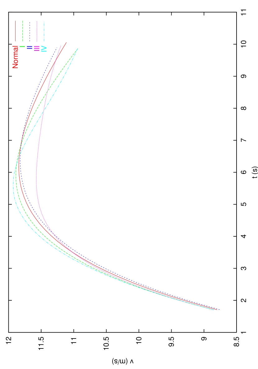
The analysis above begs the question: what kind of performance variations could be expected for a time-averaged wind speed of 0 ms-1? Table 5 demonstrates such potential discrepancies, with linear and sinusoidally-varying wind speed functions (the unrealistic step functions are omitted here). The linear winds simply range from equal-but-opposite maximum/minimum values (with 0 ms-1 occurring at the 5 s midpoint), the cosine functions begin and end at the indicated maximum and minimum, and the sine functions achieve a the maximum indicated with 0 ms-1-endpoints. Absolute maxima of 2 and 4 ms-1 are chosen.
The simulations for the 2 ms-1 absolute wind show variations between 0.034 s slower and +0.023 s faster than the actual 0 ms-1 wind-speed values of Table 1. Interestingly enough, the greatest advantage comes from a cosine wind which begins and ends as a head-wind, the form of which allows for greater acceleration through middle of the race. Conversely, the greatest disadvantage is from the equivalent negative-cosine wind. As the overall extremum of the wind increases, the differences become more acute (although note a much higher disadvantage when the wind is negative from about 30 m onward). Figure 7 presents the velocity profiles of several of these variable conditions, compared to the base case of Section 3.
6 Comparison to previous wind-correction estimates
Recently, a “back-of-the-envelope” expression for potential wind and altitude corrections was obtained in [20]:
| (9) |
Here, is the official race time (run with wind at altitude ), and the time for ms-1 at sea level. This is derived in part from Equation 7 by selecting a constant propulsive force, and an average velocity . The assumption is made that a sprinter expends roughly of his/her energy fighting drag at sea level. For non-zero , . The effects of wind are thus calculated by assuming the adjusted drag impacts the sprinter’s velocity by the ratio of forces , where is the average velocity at sea level with no wind for a race-time , with the wind/altitude-influenced velocity/time.
This ready-to-use expression provides a good match to the predictions of this model, as well as those of Dapena [17] and Linthorne [14]. Table 6 demonstrates the corrective potential of Equation (9) subject to the model parameters of Section 3. Note that the approximation becomes slightly worse for increasing absolute wind speeds, however the magnitude of these variations is less than 0.5% for ms-1. Such errors can certainly be accounted for by mis-estimations of the input variables.
The mismatch may also result from the constant velocity assumption in the derivation. The interested reader is referred to [20] for the complete derivation.
7 What would have been the 100 m world record in 1988?
On September 24th at the 1988 Seoul Olympics, Ben Johnson of Canada clocked an astounding 100 metre World Record time of 9.79 s, bettering his previous record of 9.83 s. Although this mark (and most of Johnson’s other records) were stricken from the books due to the infamous steroid scandal which followed, the Seoul mark did not reflect the true potential of this remarkable athlete. At about 15 m from the finish line, Johnson looked over his shoulder to gauge his lead over American Carl Lewis, and then raised his arm in victory as he coasted through the remained of the race. The question lingers: what would have been his World Record time, had he not “stopped” at about 85 m?
The model discussed herein can be used to obtain projections of his potential performances. Since no instantaneous velocity data is available for this race, the parameters in Equation 3 are selected to match the 10 m splits. Table 7 shows these values (obtained from [6]), along with two sample simulations. The measured wind-speed of the race was ms-1, and the modified drag area is kept as in Section 3. The elevation of Seoul is roughly that of sea level, so altitude corrections will be minimal in this case.
Effectively, Johnson could have lowered his previous record by almost 0.1s, a quantum leap in the event. Depending on the chosen parameters, the simulations predict times in the range of 9.60-9.62s, which round to about 9.73-9.75s once reaction time is included. In this case, two sets are selected to match the recorded splits, with the parameter values the same as in Section 3, except variation in the values of . The modified values are (Simulation 1), and (Simulation 2). Note that the maximum velocity of the simulations do not exceed 12 ms-1. While Johnson may have slightly topped this value in the real race, he most certainly did not achieve 13.1 ms-1, a feat periodically attributed to him [21].
In 1999, American Maurice Greene reset the World Record to 9.79 s during a race in Athens, Greece. Up to slight variations in altitude, the city is also at sea level, where the wind gauge read a calm ms-1. Adjusting this variable in the Johnson simulations, the time is scaled down to about 9.665 s (9.797 s after reaction) for Simulation 1, and 9.653 s for Simulation 2. (9.785 s after reaction). Thus, Johnson’s former World Record would have effectively been equal to the 9.79 s set in 1999 by Greene.
8 General conclusions and future considerations
The quasi-physical model considered herein provides a good match to measured split data, particularly in the drive phase of the race. The wind and altitude corrections for both men and women are consistent with those proposed by previous authors, although this models yields stronger deviations from the norm for variable wind conditions. If this type of scenario occurs in a real competition, then the times may appear much faster (or slower) than expect from the measured (time-averaged) wind.
Upon comparison with the previous theoretical estimates and complementary field studies, it is clear that this model is both a realistic representation of short-sprint races, as well as a useful tool which can assist in the physiological and biomechanical study of the sport.
A forthcoming manuscript [5] will discuss the effects of wind and altitude assistance in the 200 metre dash.
References
- [1] A. V. Hill, in Report of the 93rd Meeting, Brit. Assoc. Adv. Sci. 156 (1925)
- [2] J. B. Keller, ”A theory of competitive running”, Physics Today 43, Sept. 1973; J. B. Keller, ”Optimal velocity in a race”, Amer. Math. Monthly 81, 474 (1974)
- [3] R. Tibshirani, ”Who is the fastest man in the world?”, Amer. Stat. (May 1997)
- [4] J. R. Mureika, Can. J. Phys. 75, 837-851 (1997)
- [5] J. R. Mureika, “Simulating wind and altitude effects in the 200 metre sprint” in preparation
- [6] “Scientific Research Project at the Games of the XXIVth Olympiad - Seoul 1988”, Bruggemann, G. and Glad, B. (eds), IAAF and Charles University, Prague (1988)
- [7] Davies, C. T. M. J. Appl. Physio. 48, 702-709 (1980)
- [8] W. G. Pritchard, ”Mathematical models of running”, SIAM Review 35, 359 (1993)
- [9] N. Linthorne, personal communication. (1994)
- [10] Official 1998/1999 Handbook, International Amateur Athletics Federation, Monaco (1998)
- [11] “IAAF Biomechanics Research Project - Athens 1997”, German Sport University Cologne, Germany; Institute for Athletics (1997)
- [12] “The IAAF World Championship in Athletics, Sevilla ’99: Results of the 100 m Men”, Laboratory of Biomechanics, Consejo Superior de o Deportes (eds) (1999)
- [13] JENOPTIK Laser Systems, http:www.jenoptik-los.de
- [14] N. P. Linthorne, J. App. Biomech. 10, 110-131 (1994)
- [15] J. R. Mureika, “9.84 vs. 9.84: The Battle of Bruny and Bailey”, Athletics: Canada’s National Track and Field / Running Magazine (December 1999)
- [16] Dapena, J. and Feltner, M. E. Int. J. Sport Biomech. 3, 6-39 (1987)
- [17] Dapena, J. personal communication; also “Corrections for Wind and Altitude”, The Big Green Book, Track and Field News Press (2000)
- [18] N. P. Linthorne, “Wind and altitude assistance in the 100-m sprint”, Proceedings, Eighth Biennial Conference, Canadian Society for Biomechanics (1994)
- [19] N. P. Linthorne, “Wind speed variations at athletics tracks”, submitted to 3rd Engineering in Sport Conference
- [20] J. R. Mureika, “Back-of-the-envelope wind and altitude correction in the 100 metre dash”, submitted to the Journal of Mathematical Physics
- [21] Feschuk, D. The National Post (18 Jun 1999)
| d (m) | ms-1 | ms-1 | ||
|---|---|---|---|---|
| 10 | 1.708 | 8.800 | 1.705 | 8.840 |
| 20 | 2.747 | 10.323 | 2.738 | 10.396 |
| 30 | 3.676 | 11.142 | 3.659 | 11.240 |
| 40 | 4.554 | 11.584 | 4.529 | 11.710 |
| 50 | 5.409 | 11.792 | 5.373 | 11.941 |
| 60 | 6.254 | 11.844 | 6.208 | 12.012 |
| 70 | 7.100 | 11.787 | 7.041 | 11.970 |
| 80 | 7.953 | 11.650 | 7.880 | 11.849 |
| 90 | 8.818 | 11.455 | 8.730 | 11.666 |
| 100 | 9.700 | 11.217 | 9.596 | 11.439 |
| d (m) | 500 m | 1000 m | 1500 m | 2000 m | 2500 m | |||||
|---|---|---|---|---|---|---|---|---|---|---|
| 10 | 1.708 | 8.806 | 1.708 | 8.811 | 1.707 | 8.8148 | 1.707 | 8.820 | 1.707 | 8.8243 |
| 20 | 2.746 | 10.335 | 2.745 | 10.345 | 2.744 | 10.355 | 2.743 | 10.364 | 2.742 | 10.373 |
| 30 | 3.674 | 11.159 | 3.671 | 11.174 | 3.669 | 11.189 | 3.667 | 11.203 | 3.665 | 11.217 |
| 40 | 4.550 | 11.606 | 4.547 | 11.627 | 4.543 | 11.646 | 4.540 | 11.665 | 4.537 | 11.683 |
| 50 | 5.403 | 11.819 | 5.398 | 11.845 | 5.393 | 11.869 | 5.388 | 11.891 | 5.383 | 11.912 |
| 60 | 6.246 | 11.875 | 6.239 | 11.905 | 6.232 | 11.932 | 6.226 | 11.958 | 6.220 | 11.980 |
| 70 | 7.090 | 11.821 | 7.080 | 11.854 | 7.071 | 11.885 | 7.063 | 11.914 | 7.055 | 11.941 |
| 80 | 7.940 | 11.687 | 7.928 | 11.723 | 7.917 | 11.756 | 7.906 | 11.788 | 7.896 | 11.818 |
| 90 | 8.803 | 11.495 | 8.788 | 11.533 | 8.774 | 11.568 | 8.761 | 11.602 | 8.749 | 11.634 |
| 100 | 9.681 | 11.259 | 9.664 | 11.298 | 9.647 | 11.335 | 9.631 | 11.371 | 9.617 | 11.404 |
| d (m) | Case 1 | Case 2 | Case 3 | Case 4 | ||||
|---|---|---|---|---|---|---|---|---|
| 10 | 1.708 | 8.800 | 1.703 | 8.865 | 1.708 | 8.812 | 1.704 | 8.861 |
| 20 | 2.747 | 10.323 | 2.732 | 10.449 | 2.745 | 10.354 | 2.734 | 10.431 |
| 30 | 3.676 | 11.149 | 3.648 | 11.321 | 3.67 | 11.197 | 3.652 | 11.282 |
| 40 | 4.554 | 11.584 | 4.511 | 11.810 | 4.543 | 11.668 | 4.519 | 11.747 |
| 50 | 5.408 | 11.843 | 5.348 | 12.015 | 5.39 | 11.908 | 5.361 | 11.969 |
| 60 | 6.247 | 11.979 | 6.18 | 12.016 | 6.226 | 11.994 | 6.193 | 12.027 |
| 70 | 7.08 | 11.987 | 7.015 | 11.923 | 7.06 | 11.971 | 7.026 | 11.967 |
| 80 | 7.917 | 11.901 | 7.859 | 11.761 | 7.899 | 11.870 | 7.867 | 11.822 |
| 90 | 8.763 | 11.746 | 8.717 | 11.549 | 8.746 | 11.711 | 8.72 | 11.613 |
| 100 | 9.621 | 11.540 | 9.592 | 11.298 | 9.608 | 11.508 | 9.59 | 11.355 |
| (s) | +0.079 s | +0.108 s | +0.092 s | +0.110 s | ||||
| d (m) | Slow Start | |
|---|---|---|
| 10 | 1.765 | 8.896 |
| 20 | 2.788 | 10.486 |
| 30 | 3.705 | 11.269 |
| 40 | 4.575 | 11.677 |
| 50 | 5.423 | 11.861 |
| 60 | 6.264 | 11.896 |
| 70 | 7.107 | 11.826 |
| 80 | 7.957 | 11.681 |
| 90 | 8.821 | 11.480 |
| 100 | 9.701 | 11.238 |
| Wind (ms-1) | t (s) | (ms-1) | (m) | (s) |
|---|---|---|---|---|
| 9.690 | 11.867 | 57.534 | +0.010 | |
| 9.716 | 11.823 | 61.134 | ||
| 9.734 | 11.718 | 57.490 | ||
| 9.677 | 11.953 | 60.293 | +0.023 | |
| 9.691 | 11.885 | 55.283 | +0.009 | |
| 9.720 | 11.821 | 64.336 | ||
| 9.687 | 11.889 | 56.153 | +0.013 | |
| 9.739 | 11.803 | 63.397 | ||
| 9.778 | 11.575 | 54.359 | ||
| 9.665 | 12.043 | 61.125 | +0.035 | |
| 9.693 | 11.932 | 52.749 | +0.007 | |
| 9.752 | 11.814 | 69.150 |
| w (ms-1) | m | 1000 m | 2000 m |
|---|---|---|---|
| -5 | 9.736 | 9.730 | 9.724 |
| -4 | 9.729 | 9.724 | 9.717 |
| -3 | 9.723 | 9.716 | 9.710 |
| -2 | 9.715 | 9.709 | 9.703 |
| -1 | 9.708 | 9.702 | 9.696 |
| +0 | — | 9.695 | 9.689 |
| +1 | 9.693 | 9.687 | 9.683 |
| +2 | 9.686 | 9.681 | 9.676 |
| +3 | 9.680 | 9.676 | 9.672 |
| +4 | 9.674 | 9.671 | 9.667 |
| +5 | 9.669 | 9.666 | 9.663 |
| d (m) | Official Split | Simulation 1 | Simulation 2 | ||
|---|---|---|---|---|---|
| 10 | 1.70 | 1.698 | 8.859 | 1.698 | 8.864 |
| 20 | 2.74 | 2.730 | 10.396 | 2.729 | 10.406 |
| 30 | 3.63 | 3.652 | 11.229 | 3.650 | 11.242 |
| 40 | 4.53 | 4.523 | 11.685 | 4.520 | 11.701 |
| 50 | 5.37 | 5.370 | 11.906 | 5.365 | 11.924 |
| 60 | 6.20 | 6.207 | 11.969 | 6.201 | 11.989 |
| 70 | 7.04 | 7.043 | 11.922 | 7.036 | 11.943 |
| 80 | 7.89 | 7.886 | 11.794 | 7.878 | 11.816 |
| 90 | 8.76 | 8.740 | 11.607 | 8.730 | 11.629 |
| 100 | 9.66 | 9.611 | 11.375 | 9.599 | 11.398 |
| 9.79 s | 9.743 s | 9.731 s | |||