Inertial waves in a rotating spherical shell: attractors and asymptotic spectrum

Abstract

We investigate the asymptotic properties of inertial modes confined in a spherical shell when viscosity tends to zero. We first consider the mapping made by the characteristics of the hyperbolic equation (Poincaré’s equation) satisfied by inviscid solutions. Characteristics are straight lines in a meridional section of the shell, and the mapping shows that, generically, these lines converge towards a periodic orbit which acts like an attractor (the associated Lyapunov exponent is always negative or zero). We show that these attractors exist in bands of frequencies the size of which decreases with the number of reflection points of the attractor. At the bounding frequencies the associated Lyapunov exponent is generically either zero or minus infinity. We further show that for a given frequency the number of coexisting attractors is finite.

We then examine the relation between this characteristic path and eigensolutions of the inviscid problem and show that in a purely two-dimensional problem, convergence towards an attractor means that the associated velocity field is not square-integrable. We give arguments which generalize this result to three dimensions. Then, using a sphere immersed in a fluid filling the whole space, we study the critical latitude singularity and show that the velocity field diverges as $1/\sqrt{d}$, $d$ being the distance to the characteristic grazing the inner sphere.

We then consider the viscous problem and show how viscosity transforms singularities into internal shear layers which in general betray an attractor expected at the eigenfrequency of the mode. Investigating the structure of these shear layers, we find that they are nested layers, the thinnest and most internal layer scaling with $E^{1/3}$-scale, $E$ being the Ekman number; for this latter layer, we give its analytical form and show its similarity to vertical $\frac{1}{3}$-shear layers of steady flows. Using an inertial wave packet traveling around an attractor, we give a lower bound on the thickness of shear layers and show how eigenfrequencies can be computed in principle. Finally, we show that as viscosity decreases, eigenfrequencies tend towards a set of values which is not dense in $[0,2\Omega]$, contrary to the case of the full sphere ($\Omega$ is the angular velocity of the system).

Hence, our geometrical approach opens the possibility of describing the eigenmodes and eigenvalues for astrophysical/geophysical Ekman numbers ($10^{-10}-10^{-20}$), which are out of reach numerically, and this for a wide class of containers.

1 Introduction

Inertial waves, which propagate in rotating fluids thanks to the restoring action of the Coriolis force, can generate very singular fluid flows when they are confined in a closed container. These very special properties of inertial modes were first noticed in the theoretical work of K. Stewartson and others Stewartson & Rickard (1969); Stewartson (1971, 1972a, 1972b); Walton (1975); London & Shen (1979). They appeared again recently in numerical investigations by Hollerbach & Kerswell (1995), Rieutord (1995), Rieutord & Valdettaro (1997), Fotheringham & Hollerbach (1998) and show an even greater generality since they are also present in stratified fluids Maas & Lam (1995); Rieutord & Noui (1999) or rotating stratified fluids Dintrans et al. (1999).

The particularity of all these waves (inertial, gravity, gravito-inertial) is that their associated modes are solutions of an ill-posed boundary-value problem when they are confined in a close container: the partial differential equation is of hyperbolic or mixed type in the spatial variables. This yields all kinds of singularities. When viscosity is included, these singularities are regularized but they still play a central role in featuring the shape of inertial modes of a rotating spherical shell; in particular, they control the asymptotic limit of small diffusivities which is the relevant limit for astrophysical or geophysical applications.

The aim of this paper is to present what we believe to be the asymptotic limit of inertial modes in a spherical shell when viscosity tends to zero. In the first part of the paper we shall present the main features of the solutions of this problem when viscosity is omitted. For this purpose we examine the trajectories of characteristics in a meridional plane of the shell as if they were trajectories of a dynamical system in some configuration space. We then focus on the relation between these trajectories and the eigenfunctions in two and three dimensions. We end this part with a close look at the critical latitude singularity. In the second part we investigate the changes brought on by viscosity and we examine more closely the structure of shear layers which arise. Then, by studying the behaviour of a wave-packet, we show how eigenvalues and eigenmodes may be computed in the asymptotic limit of a small viscosity. We conclude this part by a brief discussion of the distribution of eigenvalues in the complex plane. The paper ends with a discussion of the more general cases including containers with a different shape and of the applications of the present theoretical results.

As this paper is rather long and goes through some mathematical developments which may be skipped at first reading, we suggest the casual reader to skip subsections §2.2.1-5, 2.3.1-2 and 2.4.1-2 and be lead by the introductions of sections 2.2, 2.3 and 2.4 and then jump to 2.5 and 2.6. The second part is not so mathematical but the details of the boundary layer analysis (§3.2.2-4) can be skipped at first reading.

2 Some properties of inviscid solutions

2.1 Equations of motion

We consider a fluid with no viscosity contained in a spherical shell whose outer radius is $R$ and inner radius $\eta R$ with $\eta<1$. The fluid is rotating around the $z$-axis with the angular velocity $\Omega$. Using $(2\Omega)^{-1}$ as the time scale and $R$ as the length scale, small amplitude perturbations obey the linear equation

$$\left.\begin{array}[]{l}\frac{\partial\vec{u}}{\partial t}+\vec{e}_{z}\times\vec{u}=-{\rm NewA}p\\ \\ {\rm NewA}\cdot\>\vec{u}=0\end{array}\right\}$$ (1)

where $\vec{u}$ is the velocity field of the perturbations and $p$ is the reduced pressure perturbation. The boundary conditions are simply

$$\vec{u}\cdot\vec{e}_{r}=0\qquad{\rm at}\quad r=\eta\quad{\rm and}\quad r=1$$ (2)

As in Rieutord & Valdettaro (1997) and Dintrans, Rieutord & Valdettaro (1999) we shall use spherical coordinates $(r,\theta,\varphi)$ or cylindrical coordinates $(s,\varphi,z)$. $\vec{e}_{q}$ will denote the unit vector associated with the coordinate $q\in\{r,\theta,\varphi,s,z\}$.

When the time dependence of the solutions is assumed proportional to $\exp(i\omega t)$, equations (1) may be cast into a single equation for the pressure, namely

$$\nabla^{2}p-\frac{1}{\omega^{2}}\frac{\partial^{2}p}{\partial z^{2}}=0$$ (3)

which has been referred to as Poincaré equation since the work of Cartan (1922). This equation is completed by the boundary condition $\vec{u}\cdot\vec{e}_{r}=0$ which reads

$$-\omega^{2}\vec{e}_{r}\cdot{\rm NewA}p+i\omega(\vec{e}_{z}\times\vec{e}_{r})\cdot{\rm NewA}p+(\vec{e}_{z}\cdot\vec{e}_{r})(\vec{e}_{z}\cdot{\rm NewA}p)=0$$ (4)

when expressed with the pressure; it applies at $r=\eta$ and $r=1$.

As is well-known Greenspan (1969), the Poincaré equation is hyperbolic since for all modes $\omega<1$. Therefore, a first step in the analysis of this equation is the determination of the characteristics surfaces; for this purpose, we note that second-order derivatives of this equation read

$$\frac{\partial^{2}p}{\partial x^{2}}+\frac{\partial^{2}p}{\partial y^{2}}-\frac{\alpha^{2}}{\omega^{2}}\frac{\partial^{2}p}{\partial z^{2}}$$

where $\alpha^{2}=1-\omega^{2}$. $x$ and $y$ are the cartesian coordinates in a plane $z=0$. These second-order derivatives define characteristics surfaces such as $z-f(x,y)=0$ where $f$ verifies :

$$\left(\frac{\partial f}{\partial x}\right)^{\!2}+\left(\frac{\partial f}{\partial y}\right)^{\!2}=\frac{\alpha^{2}}{\omega^{2}}\,.$$ (5)

These surfaces are known as ‘surfaces of constant slope’ as any tangent plane makes the same angle $\vartheta=\frac{\pi}{2}-\arcsin\omega$ with the equatorial plane $z=0$. In fact, these surfaces may be generated by a family of such planes or by cones which aperture angle is

$$\lambda=\arcsin\omega$$ (6)

which is also the critical latitude in a sphere. In a meridional plane, the trace of these surfaces are simply straight lines making the angle $\lambda$ with the rotation axis.

A second step in the analysis of the Poincaré equation is to examine the separability of the variables. Because of the symmetry of the problem with respect to rotations around the $z$-axis, the $\varphi$ variable may always be separated from the two others. This implies that solutions may always be expressed as

$$\sum_{m}p_{m}(r,\theta)e^{im\varphi}$$

and that each Fourier component $p_{m}(r,\theta)$ is independent of the others.

The two other coordinates, however, are not separable in the general case. This point may be understood easily if we recall that through a linear transformation of the $z$-coordinate, the Poincaré equation may be transformed into the Laplace equation as first shown by Bryan (1889) (see also Greenspan, 1969). In this transformation the boundaries transform into one-sheet hyperboloids. One therefore adopts an ellipsoidal coordinate system within which one of the boundaries is a surface of coordinate; unfortunately, since the two bounding hyperboloids are not confocal, coordinates can be only separated on one of the boundaries of the spherical shell. Hence, one may simplify, and actually solve, the problem either in the full sphere (see Greenspan, 1969) or in the infinite fluid outside a sphere (see below).

We have now seen the basic ingredients which make this problem difficult: hyperbolicity (ill-posedness) and non-separability.

2.2 Orbits of characteristics

As shown by the foregoing discussion the difficulty of the problem lies in the behaviour of the solutions with respect to the coordinates in a meridional plane $(s,z)$ or $(r,\theta)$. We shall therefore restrict our analysis to this plane where characteristic surfaces are simply straight lines; thanks to the $\exp(im\varphi)$-dependence, our results will apply equally to axisymmetric or non-axisymmetric modes. Indeed, using the separation of the $\varphi$-variable, we eliminate second-order derivatives in $\varphi$ and characteristic surfaces are just cones independent of $m$. We shall therefore study, in the following subsections, the trajectories of characteristics in a meridional plane as we did in Dintrans et al. (1999). Since this is a rather technical matter, the reader may first skip it and directly jump to section 2.3 where the results are summarized.

2.2.1 The mapping

From (5) we derive the well-known equations of the two families of characteristics:

$$\omega z\pm\alpha s=u_{\mp}$$ (7)

where $u_{\pm}$ will designate the characteristics coordinates. $u_{+}$ and $u_{-}$ are constant along characteristics of positive and negative slopes, respectively.

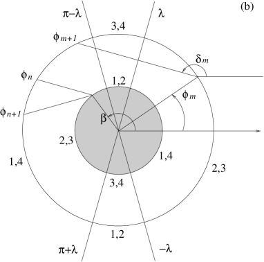
Figure 1: (a) The four directions of propagation and the corresponding four values of $\delta_{n}$’s. (b) A sketch of the notations used to describe the mapping. The numbers (1,4), (2,3) etc. indicate the possible directions of propagation of characteristics as shown in the panel (a).

To describe the paths followed by characteristics, we first study the map which relates the position of the n+1^th reflection point to the one of the n^th both taken on the outer sphere. For this purpose we mark out these points by an angle $\phi\in[0,2\pi]$ which is identical to the latitude when $0\leq\phi\leq\pi/2$; this is indeed more convenient than the colatitude. If one reflection is needed on the inner sphere then we have

$$\left.\begin{array}[]{l}\sin(\phi_{n}-\delta_{n})=\eta\sin(\beta-\delta_{n})\\ \sin(\phi_{n+1}-\delta_{n+1})=\eta\sin(\beta-\delta_{n+1})\\ \end{array}\right\}$$ (8)

where $\beta$ is the position of the reflection point on the inner shell and $\delta_{n}=\pm\pi/2\pm\lambda$ is the direction of the characteristic which can take four values as illustrated in figure 1a. If the two reflection points are simply connected by one segment of characteristics then the recurrence relation is either

$$\phi_{m}+\phi_{m+1}=-2\lambda\;[2\pi]$$ (9)

when the characteristic has a positive slope, or

$$\phi_{m}+\phi_{m+1}=2\lambda\;[2\pi]$$ (10)

when the characteristic has a negative slope. These notations are summarized in figure 1b.

From the expression (8), (9) and (10) one can compute the map

$$\phi_{n+1}=\left\{\begin{array}[]{c}f_{+}(\phi_{n})\\ f_{-}(\phi_{n})\end{array}\right.$$

Figure 2: The resulting mapping in the case of a shell with $\eta=0.35$ when the frequency is $\omega=0.40782$. Twelve points of discontinuity indicate the projection of the ‘shadow’ and the critical latitude of the inner sphere on the outer one (see text); the four apparent discontinuities due to the periodicity in the [0,4$\pi$] interval are not counted.

Such a map is bi-valued since one may compute the image by first applying a positive- ($f_{+}$) or a negative- ($f_{-}$) slope characteristic. However, such a representation is not convenient for iterating the map since for each iteration one has to decide whether to use $f_{+}$ or $f_{-}$. We therefore constructed a single-valued map which is defined in the following way: Considering a point of the outer sphere, we mark it out by the angle $\phi\in[0,2\pi]$ if it is to be iterated by $f_{-}$ or by the same angle plus $2\pi$ if it is to be iterated by $f_{+}$. We thus define the map:

$$f\,:\, [0,4\pi] \longrightarrow[0,4\pi]$$ (11)

$$\phi_{n} \longrightarrow f(\phi_{n})=\phi_{n+1}$$

which is one-to-one except at some points of discontinuity and which can be easily iterated. An example of this map is given in figure 2.

One of the remarkable features of this map is that it is not continuous. The discontinuities occur at the colatitudes (in the first quadrant)

$$\theta_{\pm}=\lambda\pm\arcsin\eta,\qquad\theta_{s}=\lambda+\arcsin(\eta\cos 2\lambda)$$

$\theta_{\pm}$ are delineating the ‘shadow’ projection of the inner shell on the outer shell (see figure 5 for an illustration of the shadow). They illustrate the case when a characteristic is tangent to the inner sphere at critical latitude. $\theta_{s}$ is the colatitude of the projection of the inner sphere’s critical latitude on the outer sphere. These angles ($\theta_{\pm}$) delimit the intervals where the map is contracting $|f^{\prime}|<1$ or dilating $|f^{\prime}|>1$ or neutral $|f^{\prime}|=1$.

When the map (11) is iterated as in figure 3 and since, generically, discontinuities are not mapped onto themselves, their number increases proportionally to the number of iterations; also some fixed points appear which indicate the existence of attractors, i.e. attractive periodic orbits which we discuss below (§2.2.4). We would therefore expect that the basins of attraction of the infinitely iterated map, containing an infinite number of intervals at smaller and smaller scales, would have a fractal structure; however, numerical studies show only isolated accumulation points which are actually the fixed repulsive points of the mapping, i.e. the repellors (see figure 4).

We therefore see that the structure of basins of attraction is much more complicated than in the case studied by Maas & Lam (1995) and may represent the general case for such systems.

Figure 3: The third (left panel) and eighth (right panel) iterate of the map in the case of a mode with $\omega=0.40782$ for a shell of aspect ratio $\eta=0.35$: note the appearance of fixed points marked out by the intersection of the curve with the line $\phi_{n+p}=\phi_{n}$. They indicate the existence of attractive periodic orbits of period 3 and 8 respectively. Note also the increased number of discontinuities of the mapping.

Figure 4: Zoom of the $N^{\rm th}$ iterate ($N=1200$) of the map near an accumulation point. The aspect ratio $\eta$ and the frequency $\omega$ are the same as in figure 3. On the left panel we clearly see the presence of the accumulation point $\phi^{R}$; the two arrows indicate the basins of attraction of the polar attractor in figure 7a; the other segments belong to the basin of the other (equatorial) attractor. On the right panel we see that the width of the intervals of the basins of attraction vanishes geometrically as the accumulation point is approached.

2.2.2 Orbits and Lyapunov exponents: the full sphere case

Once the mapping is known, we may examine the trajectories of characteristics. For the sake of clarity, it is useful to first consider the case of the full sphere for which only (9) and (10) are necessary.

We first note that the number of reflection points of a periodic orbit is necessarily even, i.e. $2q$, when the starting point is not a critical latitude. Applying alternatively (9) and (10), we have

$$\left.\begin{array}[]{l}\phi_{1}=-\phi_{2}+2\lambda\;[2\pi]\\ -\phi_{2}=\phi_{3}+2\lambda\;[2\pi]\\ \vdots\qquad\vdots\qquad\vdots\\ \phi_{2q-1}=-\phi_{2q}+2\lambda\;[2\pi]\\ -\phi_{2q}=\phi_{1}+2\lambda\;[2\pi]\end{array}\right\}$$ (12)

Summing all these equations leads to the conclusion that a periodic orbit is such that

$$\lambda=\frac{p\pi}{2q}$$ (13)

where $p$ and $2q$ are integers which represent the number of crossings of the orbit with respectively the axis of rotation or the equator.

From the preceding results, it turns out that all orbits such that $\lambda=r\pi$ with $r$ irrational, are ergodic (quasi-periodic). At this point it is worth noting that eigenfrequencies of inertial modes in the full sphere are in general associated with quasi-periodic orbits. We prove in appendix A that, for instance, the first axisymmetric inertial mode of frequency $\sqrt{3/7}$ is associated with a quasi-periodic orbit.

To conclude with the full sphere, we just need to point out that thanks to relations (9) or (10), it is clear that the Lyapunov exponent is always zero. Indeed, if we recall the definition of the Lyapunov exponent $\Lambda$ associated with an orbit:

$$\Lambda=\lim_{N\rightarrow\infty}\frac{1}{N}\sum_{n=1}^{N}\ln\left|\frac{d\phi_{n+1}}{d\phi_{n}}\right|,$$

it is clear that for the full sphere $\left|\frac{d\phi_{n+1}}{d\phi_{n}}\right|=1\;\forall n$, so $\Lambda=0$.

Figure 5: The shadow pattern for a spherical shell with $\eta=0.2$ when $\lambda=\pi/6$ ($\omega=0.5$).

2.2.3 Orbits and Lyapunov exponents: the shell case

We now turn to the shell case. As we already observed the map has discontinuities defined by the shadow of the inner sphere on the outer shell and the projection of critical latitudes. If the inner sphere is sufficiently small, the shadow may draw a periodic pattern if the critical latitude $\lambda$ is commensurable with $\pi$. A simple case is illustrated in figure 5. For these frequencies, orbits starting in the shadow remain in the shadow while those starting outside remain outside. In this way, one can construct the set of all periodic orbits with $\Lambda=0$ i.e. all neutral periodic orbits.

The fact that periodic orbits outside the shadow are neutral is obvious; the case of orbits in the shadow is less obvious but we may consider the fact that if these orbits were not neutral, the shadow would not map onto itself. As a short exercise, we may follow one such orbit for $\omega=\sin(\pi/2(2p+1))$. The shadow should cross only twice the location of the inner sphere. It bounces first on the inner sphere, at an angle $\beta_{1}$, and then on the outer sphere at the angle $\phi_{1}$ given by $\sin(\phi_{1}-\delta)=\eta\sin(\beta_{1}-\delta)$ ($\delta$ is one of the angles $\delta_{n}$ in figure 1). Then it bounces $2p$ times on the outer sphere. After each two reflections, the angle $\phi$ changes into $\phi+4\delta$. Therefore after $2p$ bounces, the angle on the outer sphere is $\phi_{1}+4p\delta$. It bounces then again on the inner sphere, hitting it at the angle $\beta_{2}$ such that $\sin(\phi_{1}+\delta+4p\delta)=\eta\sin(\beta_{2}+\delta)$. But $2(2p+1)\delta=\pi$ therefore $\delta+4p\delta=\pi-\delta[2\pi]$. So $\sin(\phi_{1}-\delta)=-\eta\sin(\beta_{2}+\delta)=\eta\sin(\beta_{1}-\delta)$. Therefore $\beta_{1}=-\beta_{2}[2\pi]$ or $\beta_{1}=\pi+\beta_{2}+2\delta[2\pi]$. Repeating this entire process $2(2p+1)$ times, one comes back to the original $\beta_{1}$.

In fact periodic orbits of the shadow do not exist for all $\lambda$’s commensurable with $\pi$. Indeed the image of the shadow must not be split by discontinuities; this implies that $p$ or $q$ cannot be too large or the shell too thin. More precisely, for a given $\eta$, periodic orbits of the shadow exist if:

$$\arcsin\eta\leq\lambda\leq\arccos\eta$$ (14)

If $\eta\geq 1/\sqrt{2}$, only one neutral periodic orbit exists: it is such that $\lambda=\pi/4$ or $\omega=1/\sqrt{2}$. More generally, for a given aspect ratio $\eta$, one may determine all the frequencies associated with neutral periodic orbits and their number increases as the size of the inner shell decreases. These frequencies are obviously determined by (13) but due to the finite size of the shadow, one needs to eliminate large values of $p$ and $q$. If we remark that the most robust periodic orbits (when $\eta$ increases) are those with $p=1$ (restricting ourselves to $\lambda\leq\pi/4$), relation (14) easily bounds the permitted values of $q$. For a shell like the core of the Earth, where $\eta=0.35$, only $q=2,3,4$ are possible.

The frequencies of neutral periodic orbits are important as they shape the form of the Lyapunov exponent curve since, then, intervals contracting through $f_{+}$ are exactly dilated by $f_{-}$ which makes the Lyapunov exponent vanish. As a consequence, frequencies in the neighbourhood of one such frequency are associated with very long orbits having a small Lyapunov exponent. This is the reason why ‘windows’ appear near these frequencies, especially near $\omega=1/\sqrt{2}$ ($\lambda=\pi/4$) as clearly shown in figure 6.

Figure 6: The lyapunov exponent of one basin as a function of frequency (left) or critical latitude (right). Note the symmetry of this last plot with respect to $\pi/4$. The vertical dotted lines mark the critical latitudes $\pi/6$, $\pi/4$ and $\pi/3$; the aspect ratio of the shell is $\eta=0.35$.

This latter figure shows many spikes which in fact betray the presence of other periodic orbits which we shall call attractors after Maas & Lam (1995). For such orbits $\Lambda\leq 0$. In fact for this system, all the orbits (except may be some isolated ones) verify this inequality and no chaos is possible: the configuration space being one-dimensional and the mapping being one-to-one.

2.2.4 Some properties of attractors in the shell

In order to make the dynamics of attractors clearer, it is useful to concentrate on a specific example which can be computed explicitly. For this purpose, we choose a spherical shell similar to that of the core of the Earth for which $\eta=0.35$ and we focus on the orbit with four reflections on the outer or inner shell as shown in figure 7. If the shell is thinner, this orbit is localized in the vicinity of the equator which is the kind studied by Stewartson (1971, 1972a, 1972b).

Figure 7: (a) Two attractors coexisting when $\omega=0.4051$; we call them ‘polar’ and ‘equatorial’ respectively as they are characterized by the fact that the reflection on the inner sphere occurs above or below the critical latitude; the arrows indicate the direction of focusing. (b) Lyapunov exponent as a function of frequency in the vicinity of $\omega=0.4051$; the thick solid line denotes the equatorial attractor while the thick dashed line represents the polar attractor; these two thick lines have been derived from the analytic formulae (59) and (63) given in appendix B.

The Lyapunov exponent of this orbit may be computed explicitly in the following way: Let us first recall that plane inertial waves reflecting on a surface oriented by $\vec{n}$ verifies the relation

$$\vec{k}_{i}\times\vec{n}=\vec{k}_{r}\times\vec{n}$$

where $\vec{k}_{i}$ and $\vec{k}_{r}$ are the wave vectors of the incident and reflected waves respectively Greenspan (1969). When applied to a reflection on a sphere, this relation implies

$$k_{r}=k_{i}\frac{\sin(\phi\pm\lambda)}{\sin(\phi\mp\lambda)}$$

where $\phi$ is the ‘latitude’ of the reflection point. From this relation, we can compute the rate of contraction of an infinitesimal interval in the neighbourhood of a reflection point of the orbit. Therefore, the Lyapunov exponent of an attractor with $N$ reflection points is simply given by:

$$\Lambda=-\frac{1}{N}\ln\prod_{k=1}^{N}\frac{\sin(\phi_{k}\pm\lambda)}{\sin(\phi_{k}\mp\lambda)}$$ (15)

where the $\phi_{k}$’s describe the reflection points of the attractor (a periodic orbit). At this point we shall define two useful quantities characterizing attractors, namely their length and their period. We shall call the number of reflection points (on both spheres) the length of the attractor while its period will refer to the minimum number of iteration of the mapping needed to generate its associated fixed points; because of the definition of the mapping, the period is also the number of reflection points on the outer sphere. For instance, the period of the equatorial attractor of figure 7a is ’3’ and its length is ’4’, while for the polar one, the length is ’10’ and the period ’8’ (we do not allow reflections on the axis). We give in appendix B the explicit calculations relevant to the orbits of figure 7.

The curves $\Lambda(\omega)$ (figure 7b) show the same feature: in the interval of existence of the orbit, $\Lambda$ varies between 0 and $-\infty$. The two extremes correspond respectively to the cases when the reflection on the inner shell occurs at the equator or at its critical latitude. We note that the vanishing value of the Lyapunov exponent does not mean that for this frequency the orbit is no longer an attractor: it simply means that convergence towards the attractor is no longer exponential; in most cases, it does converge, but algebraically.

For later use, we also computed the behaviour of $\Lambda(\omega)$ in the vicinity of the point $\omega_{0}$ such that $\Lambda(\omega_{0})=0$. We find in the particular case of the equatorial attractor that

$$\Lambda(\omega)=-K(\omega-\omega_{0})^{1/2},\qquad{\rm with}\quad K=4.8184,\quad\omega_{0}=0.403112887$$ (16)

In fact this behaviour is general as is shown in appendix B. Let us also emphasize that when $\Lambda=0$, the orbit is just one broken line connecting:

• the equator or the pole of the spheres to another equator or pole,

• the equator or the pole of the spheres to the critical latitudes of the outer sphere.

With the terminology in use for dynamical systems, such an orbit restricted to the first quadrant is self-retracing: a mass-point would go back and forth on the same trajectory.

The foregoing results make the shape of figure 6 quite clear now. Most of the ‘spikes’ shown in this graph will therefore tend to $-\infty$ as the number of points of the graph is increased. But to be complete, we need also mention some cases when a segment of an orbit intercepts the inner shell after being tangential to it. In this case the curve $\Lambda(\omega)$ has a discontinuity and does not reach $-\infty$.

We therefore see that attractors are featuring figure 6. As it will be clear later they also feature the shape of the asymptotic spectrum. It is thus interesting to know some elementary properties of these geometrical objects.

From a rather large number of computations we observed, as Maas & Lam (1995), that, in the first quadrant, not more than two attractors may coexist for a single frequency. However, these two attractors can be used to construct other attractors which are just their image symmetrized with respect to axis of rotation and equator. Considering the propagation of characteristics in the full meridional section of the shell, we observe that these lines can converge towards six attractors at most. Using the properties of the mapping (11), we have been able to prove under certain hypotheses (see appendix C), that the number of attractors is bounded by the number of points of discontinuity (which is twelve).

We also computed the interval of existence, in frequency space, of a large number of attractors so as to show its relation with the length of the attractor. As shown in figure 9, the interval of existence is well correlated with the inverse square of the length. We explain this law in the following way: for a very long attractor of length $N\gg 1$ the number of reflections on the inner and outer shell scales with $N$, therefore the mean angular distance between the critical latitude and the nearest reflection point is ${\cal O}(1/N)$. This implies that just a ${\cal O}(1/N^{2})$ variation in frequency is necessary to shift this point to the critical latitude.

The latter result has an interesting consequence on the shape of the curve $\Lambda(\omega)$ for a given long attractor. Indeed, from (15) the divergence toward $-\infty$ of an attractor of length $N$ is of the form:

$$\Lambda\sim\frac{1}{N}\ln\left[N(\omega-\omega_{c})\right]$$

where $\omega_{c}$ is the frequency of the singularity of $\Lambda$; we used the fact that (15) is dominated by one term ( $\phi_{k}-\lambda\sim 0$ with $\phi_{k}-\lambda\sim N(\omega-\omega_{c})$ ); since the interval of existence of the attractor scales like $1/N^{2}$, if we choose a point such that $\omega-\omega_{c}=\alpha/N^{2}$ the Lyapunov exponent will scale like $\Lambda\sim-{\ln(\alpha N)\over N}$ which vanishes at large $N$. This means that the singularity of the Lypaunov curve occupies a smaller and smaller fraction of the interval of existence of the attractor. Hence for long attractors, the Lyapunov exponent is very small in a larger and larger part of their interval of existence. This explains why long attractors appear numerically as weakly attracting eventhough their Lyapunov exponent may diverge.

In figure 9 we show the distance of attractors to the point on the external sphere at critical latitude as a function of the length. Since a periodic orbit exists in a range of frequencies (see figure 9), instead of showing a single point we represent a vertical segment connecting the minimum and maximum distance over the entire range of existence of the attractor in frequency space. We see that the maximum distance is well correlated with the inverse square of the length. This distance is important in the final appearance of the attractor when viscosity is included. As it will be shown later on an example, the build-up of energy along an attractor can be impeded by the boundaries; this effect therefore puts an upper bound on the viscosity for the attractor to be visible. The dashed line in the figure gives the lower bound (in distance) for physically relevant attractors (see discussion and the example in §3.1).

Figure 8: Interval of existence in latitude of several different attractors, plotted as a function of their length $N$ The straight solid line is the inverse square of the length.

Figure 9: Distance to the point on the external sphere at critical latitude, for several different attractors, plotted as a function of the length $N$. The straight solid line is the inverse square of the length. The dashed line gives the lower bound (in distance) for physically relevant attractors (see discussion in §3.1).

2.2.5 Differences with billiards

It is interesting to compare the mapping defined by (8-10) with the billiard problem studied in classical chaos, where a particle bounces specularly on the walls of a cavity. Billiard phase spaces are two-dimensional (position and velocity direction) while the phase space of our problem is one-dimensional (in projection), since the only variable is the position along the circles representing inner and outer shells. The problem is not Hamiltonian, there is no conservation of the symplectic measure in phase space, and attractors and repellors exist.

For the full sphere, $\eta=0$, we have seen that all the orbits are neutral ($\Lambda=0$) and are either quasiperiodic (and ergodic) or periodic (when $\lambda$ is a rational fraction of $\pi$). When $\eta$ is made nonzero, all quasiperiodic orbits are instantaneously destroyed, and the periodic orbits remain neutral until they are eventually destroyed when $\eta$ increases, the rational values with smaller denominator surviving last. It is interesting to note that this situation is exactly the opposite of the Kolmogorov-Arnold-Moser (KAM) theorem valid for Hamiltonian systems close to integrability (see Arnold, 1989). In this latter case, it is well-known that for an integrable Hamiltonian system all orbits lie on tori, and orbits are organized in families, either quasiperiodic (and ergodic) or periodic, for a given torus. If one perturbs such an integrable Hamiltonian system by a sufficiently smooth perturbation, the KAM theorem states first that all rational tori (with periodic orbits) are instantaneously destroyed, and second that irrational tori (with quasiperiodic orbits) disappear one after the other when the perturbation is increased, the last to disappear being the ‘furthest’ to the rationals.

2.3 Relations between orbits of characteristics and eigenfunctions

In the preceding subsections we have shown that, generically, characteristics converge towards attractors which are formed by a periodic orbit. These attractors live in a frequency band whose size decreases with the length (or period) of the attractor. The attracting power is measured by a negative Lyapunov exponent which generically varies between 0 and $-\infty$ when the frequency band is scanned. Several (less than 6) attractors may coexist for a given frequency; in this case they own each a basin of attraction (described for instance as a set of points on the outer boundary) whose structure is governed by accumulation points (see fig. 4).

We have also found periodic orbits which are not attractors; their frequency can be written $\omega=\sin(p\pi/2q)$ where $(p,q)$ are chosen in a finite set of integers. The number of these orbits is therefore finite but increases as the radius of the inner core decreases. The frequencies of these orbits will prove to be useful since in their neighbourhood, attractors have very great length and, therefore, very small (in absolute value) Lyapunov exponents. This will influence the shape of the asymptotic spectrum (i.e. with low viscosities).

Now we shall see how the eigenfunctions are influenced by the presence of an attractor.

2.3.1 The two-dimensional case

Because of the simple form of the Poincaré equation in two dimensions, which may be written as

$$\frac{\partial^{2}P}{\partial u_{+}\partial u_{-}}=0$$ (17)

early investigations have focused on this case in particular those of mathematicians. The relevant contributions are those of Bourgin & Duffin (1939), John (1941), Høiland (1962), Franklin (1972), Ralston (1973) and Schaeffer (1975). Much of this previous work is concentrated in a theorem demonstrated in Schaeffer (1975) which states that:

There are non-trivial solutions of (17) if and only if there exists an integer n such that all reflected rays close after precisely 2n reflections. If there is one solution, then there are infinitely many, linearly independent solutions.

In other words, eigenvalues of regular modes are always associated with periodic orbits and these eigenvalues are always infinitely degenerate. Since the reflected rays must close, starting from any point of the curve, the Lyapunov exponent of such periodic orbits is always zero. Note the difference with the three-dimensional case where eigenmodes in the full sphere are associated with ergodic (quasi-periodic) orbits (cf §2.2.2 and appendix A) and eigenvalues are non-degenerate.

Another interesting result was derived from mathematical analysis by Ralston (1973). Namely, it states that the velocity field associated with a solution of (17) is not square-integrable when characteristics are focused towards a wedge formed by the boundaries. An example of such a singular flow is given in Wunsch (1968) with the case of internal waves focused by a sloping boundary. In the interval of frequencies where the velocity field is not square-integrable, eigenvalues do not exist and the point spectrum of Poincaré operator is said to be empty.

The foregoing results may be generalized to our case, or the one studied by Maas & Lam (1995), where characteristics are focused towards an attractor. Indeed, let us consider the total kinetic energy of a ‘mode’ associated with an attractor; using characteristic coordinates, this quantity reads

$$I=\int_{S}\|\vec{v}\|^{2}du_{+}du_{-}+\int_{CS}\|\vec{v}\|^{2}du_{+}du_{-}$$

where $S$ designates a neighbourhood of the attractor and $CS$ the remaining ‘volume’; we assume that the limits of $S$ are made up of characteristics. If the attractor is of length $N$ then this integral can be split into $N$ pieces

$$I=\sum_{n=1}^{N}\int_{S_{n}}\|\vec{v}\|^{2}du_{+}du_{-}$$

where we neglected the contribution from $CS$. Now each of these pieces can be split again into an infinite number of rectangles $R_{k}$ with sides made up of characteristics. Hence we write

$$\int_{S_{n}}\|\vec{v}\|^{2}du_{+}du_{-}=\sum_{k=1}^{\infty}\int_{R_{k}}\|\vec{v}\|^{2}du_{+}du_{-}=\sum_{k=1}^{\infty}I_{k}$$

In the vicinity of the attractor, these rectangles are very elongated: one side remains ${\cal O}(1)$ long while the other shrinks to zero as the attractor is approached.

Now we take the two long sides as images through the mapping made by the characteristics. The mapping has a contracting rate given by $e^{\Lambda}<1$ where $\Lambda$ is its Lyapunov exponent. Maas & Lam (1995) have shown how one can construct the stream function in the whole domain by iterating an arbitrary function given on its boundary. When the attractor is approached, the scale of the stream function vanishes while its amplitude remains constant; therefore the kinetic energy is amplified by a factor $e^{-2\Lambda}$ at each iteration of the mapping. Noting that one rectangle is smaller by a factor $e^{\Lambda}$ than its predecessor, we can derive the iteration rule

$$I_{k+1}=e^{-\Lambda}I_{k}$$

which shows that the integral $I$ is infinite. We may note in passing that if $d_{k}$ is the distance of the $k^{\rm th}$ characteristic to the limit cycle, then $d_{k}=d_{0}e^{k\Lambda}$ while the amplitude of the velocity field is $v_{k}=v_{0}e^{-k\Lambda}$. This shows that the velocity field diverges as the inverse of the distance to the attractor.

Therefore, as in the case of a wedge, the velocity field is not square-integrable when characteristics converge towards an attractor.

2.3.2 The three-dimensional case

The 3-D case has not benefitted from the same interest by mathematicians. In this case the Poincaré equation contains first or zeroth order derivatives which cannot be eliminated. Let us rewrite it using cylindrical coordinates and assume a exp$(im\varphi)$ dependence of the pressure; thus

$$\frac{\partial^{2}P}{\partial s^{2}}+\frac{1}{s}\frac{\partial P}{\partial s}-\frac{\alpha^{2}}{\omega^{2}}\frac{\partial^{2}P}{\partial z^{2}}-\frac{m^{2}P}{s^{2}}=0$$

The canonical form of this equation is obtained using characteristics coordinates:

$$2\frac{\partial^{2}P}{\partial u_{+}\partial u_{-}}-\frac{1}{u_{+}-u_{-}}\left(\frac{\partial P}{\partial u_{+}}-\frac{\partial P}{\partial u_{-}}\right)-\frac{m^{2}}{(u_{+}-u_{-})^{2}}P=0$$ (18)

which is known as the Euler-Darboux equation Dautray & Lions (1984-1985).

\psfrag{M}{S}\psfrag{P}{P}\psfrag{Q}{Q}\psfrag{S}{\hskip 2.84526pt\raisebox{-1.13809pt}{M}}\psfrag{X}{\raisebox{0.56905pt}{$\bullet$}}\psfrag{s}{$s$}\psfrag{z}{$z$}\includegraphics[width=270.30118pt,angle={0}]{fig/rieman.eps}

Figure 10: A sketch for the illustration of Riemann’s method; the lines (SP) and (SQ) are segments of characteristics.

A general solution of Euler-Darboux equation may be obtained with Riemann’s method Colombo (1976); Zwillinger (1992). With this method one may express the value of the solution at one point when ‘initial’ data are given on an arc joining two points on characteristics ‘emitted’ from the point considered (see figure 10). However, one needs to know the Riemann function (which plays an equivalent role to the Green’s function of elliptic problems). To determine this function it is useful to rewrite the pressure fluctuation as $P=\Pi/\sqrt{s}$; doing so, the first derivatives of Poincaré equation are eliminated but are replaced by the term $\Pi/4s^{2}$. The equation for $\Pi$ is therefore:

$$\frac{\partial^{2}\Pi}{\partial u_{+}\partial u_{-}}+\left(m^{2}-\frac{1}{4}\right)\frac{\Pi}{(u_{+}-u_{-})^{2}}=0$$ (19)

The Riemann function is a solution of this equation which meets the additional conditions:

$$R(u_{+},u_{-})=1,\qquad\left.\frac{\partial R}{\partial u_{+}}\right)_{u_{-}}=\left.\frac{\partial R}{\partial u_{-}}\right)_{u_{+}}=0$$ (20)

or, equivalently,

$$R(u^{\prime}_{+},u_{-})=R(u_{+},u^{\prime}_{-})=1\qquad\forall(u^{\prime}_{+},u^{\prime}_{-})\in{\cal D}$$

We shall call $S(u_{+},u_{-})$ the point where the solution is computed and $M(u^{\prime}_{+},u^{\prime}_{-})$ a point running on the arc of data; ${\cal D}$ is the area defined by (SPQ).

As Friedlander & Heins (1968) have noted, (19) is invariant for all the transformations leaving

$$z=\frac{(u^{\prime}_{+}-u_{+})(u^{\prime}_{-}-u_{-})}{(u^{\prime}_{+}-u^{\prime}_{-})(u_{+}-u_{-})}$$

invariant. Therefore, seeking a solution of the form $R(z)$, one finds that this function verifies the differential equation:

$$z(1-z)R^{\prime\prime}-(2z-1)R^{\prime}+\mu(\mu-1)R=0$$

where we set $\mu=m+1/2$. This is a special case of the differential equation of Gauss hypergeometric function, i.e. $F(\mu,1-\mu;1;z)$; in fact, it is just the equation satisfied by Legendre functions of index $\mu-1$.

Since $z\equiv z(S,M)$, we shall write Riemann’s function as $R(S;M)$. Hence the formal solution of the problem is

$$\Pi(S)=\frac{1}{2}(\Pi(P)+\Pi(Q))$$

$$+\frac{1}{2}\int_{PQ}R(S;M)\left(\frac{\partial\Pi}{\partial u_{+}}du_{+}-\frac{\partial\Pi}{\partial u_{-}}du_{-}\right)+\Pi(M)\left(\frac{\partial R}{\partial u_{+}}du_{+}-\frac{\partial R}{\partial u_{-}}du_{-}\right)$$ (21)

which shows how the value of $\Pi$ at $S$ may be constructed from the data given on the arc $PQ$.

A simpler formula can be obtained for axisymmetric modes when the meridional stream function $\psi$ is considered. After a similar transformation, where we set $\psi=\sqrt{s}\Psi$, we find that the associated Riemann function is also a Legendre function with $\mu=-1/2$. If the arc $PQ$ is taken on the boundary then $\Psi=0$ and the expression (21) simplifies into

$$\Psi(S)=\frac{1}{2}\int_{PQ}R(S;M)\left(\frac{\partial\Psi}{\partial u_{+}}du_{+}-\frac{\partial\Psi}{\partial u_{-}}du_{-}\right)$$ (22)

Let us now suppose that $S$ is also on the boundary (on the inner sphere for instance); then $\Psi(S)=0$. If we introduce $d{\cal C}(\Psi)=\left(\frac{\partial\Psi}{\partial u_{+}}du_{+}-\frac{\partial\Psi}{\partial u_{-}}du_{-}\right)$, then we have

$$\int_{PQ}R(S;M)d{\cal C}(\Psi)=0$$

This relation holds also for neighbouring points $(P^{\prime}Q^{\prime}S^{\prime})$ of $(PQS)$, thus

$$\int_{P^{\prime}Q^{\prime}}R(S^{\prime};M)d{\cal C}(\Psi)=0$$

By subtracting these two equations we get

$$\int_{PP^{\prime}}R(S;M)d{\cal C}(\Psi)+\int_{QQ^{\prime}}R(S;M)d{\cal C}(\Psi)+d\phi_{S}\int_{PQ}\frac{\partial R}{\partial\phi}(S;M)d{\cal C}(\Psi)=0$$ (23)

where $d\phi_{S}$ denotes the variation of the position of $S$. Since $P^{\prime}$ and $Q^{\prime}$ are in a neighbourhood of $P$ and $Q$ respectively and that $R(S;P)=R(S;Q)=1$, the first integrals of (23) can be simplified so that:

$${\cal C}(\Psi)(P)+{\cal C}(\Psi)(Q)+\frac{d\phi_{S}}{d\phi}\int_{PQ}\frac{\partial R}{\partial\phi}(S;M)d{\cal C}(\Psi)=0$$ (24)

where ${\cal C}(\Psi)=\frac{\partial\Psi}{\partial u_{+}}\frac{\partial u_{+}}{\partial\phi}-\frac{\partial\Psi}{\partial u_{-}}\frac{\partial u_{-}}{\partial\phi}$.

Now we consider that $PSQ$ are part of a limit cycle like the one of figure 7a (right); let us call $T$ the fourth point of this cycle and let $P_{n},S_{n},Q_{n},T_{n}$ be the suite of points converging towards $PSQT$ (i.e. those points at $(\phi_{3},\phi_{4},\phi_{1},\phi_{2})$ respectively). (24) can be applied to the triangles $P_{n},S_{n},Q_{n}$ and $Q_{n},T_{n},P_{n+1}$ and we get:

$${\cal C}(\Psi)(P_{n})={\cal C}(\Psi)(P_{n+1})+\frac{d\phi_{T}}{d\phi}\int_{Q_{n}P_{n+1}}\frac{\partial R}{\partial\phi}(T_{n},M)d{\cal C}(\Psi)+\frac{d\phi_{S}}{d\phi}\int_{Q_{n}P_{n}}\frac{\partial R}{\partial\phi}(S_{n},M)d{\cal C}(\Psi)$$

The two integrals in the RHS are of order unity and we surmise that they do not cancel. Therefore the suite of ${\cal C}(\Psi)(P_{n})$ is diverging which means that the velocity fields tends to infinity when a limit cycle is approached.

This result can be generalized to any limit cycle. We may also use it to generalize Ralston’s theorem. However, in this latter case, it is more straightforward to note that if we are considering characteristics converging towards a wedge (for a three-dimensional problem), then in a neighbourhood of the apex of the wedge, first order derivatives are negligible compared to second order derivatives; therefore, in this neighbourhood, (18) can be transformed into (17) and Ralston’s theorem applies.

2.4 The critical latitude singularity

The preceding discussion has shown (and proved in 2D) that the velocity field of ‘modes’ associated with an attractor is not square-integrable: it diverges as the inverse of the distance to the attractor.

We shall see now that this singularity is not the only one and that a milder one develops around the critical latitude of the inner sphere. Stewartson & Rickard (1969) were the first to notice that singularity and showed that it is integrable. Although the work of Stewartson & Rickard (1969) was restricted to the thin shell limit and was based on the use of Longuet-Higgins solutions of the Laplace tidal equation, we shall show that their result is in fact general.

For quick reading demonstrations in §2.4.1 and §2.4.2 can be skipped.

2.4.1 The singular surfaces

Let us consider a sphere immersed in a rotating fluid filling the whole space. We examine the oscillations of the fluid. Such modes are the corresponding modes of the full sphere when solutions regular at the origin are replaced by solutions regular at infinity.

As for the full sphere, we use Bryan’s transformation to convert the Poincaré equation into the Laplace equation. Thus we set

$$z^{\prime}=-i\frac{\omega}{\alpha}z$$

To solve Laplace’s equation, we therefore use ellipsoidal coordinates $(\xi,\theta,\varphi)$ similar to the spherical coordinates (for the angular variables $\theta$ and $\varphi$):

$$\left.\begin{array}[]{l}x=a\cosh\xi\sin\theta\cos\varphi\\ y=a\cosh\xi\sin\theta\sin\varphi\\ z^{\prime}=a\sinh\xi\cos\theta\end{array}\right\}$$ (25)

where $a$ is the focal distance of the meridional ellipse. If we take the radius of the sphere as the unit of length, then $a=1/\alpha$. We recall that using these coordinates, Laplace equation of an axisymmetric field transforms into :

$$\nabla^{2}V=\frac{1}{\cosh\xi}\frac{\partial}{\partial\xi}\left(\cosh\xi\frac{\partial V}{\partial\xi}\right)+\frac{1}{\sin\theta}\frac{\partial}{\partial\theta}(\sin\theta V)=0$$ (26)

whose solution, regular at infinity, reads:

$$Q_{\ell}(i\sinh\xi)P_{\ell}(\cos\theta)$$ (27)

where $Q_{\ell}$ is the second-kind Legendre function.

If we now come back to the original coordinates, we may write the cylindrical coordinates $(s,z)$ as

$$\left.\begin{array}[]{l}\displaystyle s=\frac{1}{\alpha}\cosh\xi\sin\theta\\ \\ \displaystyle z=\frac{i}{\omega}\sinh\xi\cos\theta\end{array}\right\}$$ (28)

and following the idea of Greenspan (1969), we introduce

$$\mu=\cos\theta\qquad{\rm and}\qquad\eta=i\sinh\xi$$ (29)

so that

$$\left.\begin{array}[]{l}\alpha s=\sqrt{(1-\mu^{2})(1-\eta^{2})}\\ \omega z=\mu\eta\end{array}\right\}$$ (30)

The Jacobian of this new coordinate transform is

$$J=\frac{\alpha^{2}\omega s}{\eta^{2}-\mu^{2}}$$ (31)

where we used

$$\left.\begin{array}[]{l}\frac{\partial\mu}{\partial s}=\frac{\alpha^{2}s\mu}{\Delta},\qquad\frac{\partial\mu}{\partial z}=\frac{\omega(1-\mu^{2})\eta}{\Delta}\\ \\ \frac{\partial\eta}{\partial s}=-\frac{\alpha^{2}s\eta}{\Delta},\qquad\frac{\partial\eta}{\partial z}=-\frac{\omega\mu(1-\eta^{2})}{\Delta}\end{array}\right\}$$ (32)

with $\Delta=\eta^{2}-\mu^{2}$. Hence, the transform is singular on the surfaces such that $\eta=\pm\mu$. Since the solution $Q_{\ell}(\eta)P_{\ell}(\mu)$ is regular in the fluid’s domain, the singularity of the transformation makes the solutions singular when the coordinates map the space in a regular way.

To discover which kind of surfaces hinds behind this equation ($\eta=\pm\mu$), it is convenient to express $\xi$ (or $\eta$) as a function of the cylindrical coordinates $s$ and $z$. Eliminating $\theta$ from (28) and setting $X=\sinh^{2}\xi$, we find that

$$X^{2}+(1+\omega^{2}z^{2}-\alpha^{2}s^{2})X+\omega^{2}z^{2}=0$$

The solution of this equation gives the reciprocal transformation of coordinates (30) or (28). When the roots are multiple, the transformation is singular; this happens when the discriminant $D$ vanishes which is when

$$D=(1-\omega z-\alpha s)(1-\omega z+\alpha s)(1+\omega z+\alpha s)(1+\omega z-\alpha s)=0$$ (33)

One may easily verify that this equation is equivalent to $\eta^{2}=\mu^{2}$.

We have therefore shown that the transformation is singular on four surfaces which are cones tangent to the sphere at the critical latitudes. This result is summarized in figure 11.

\psfrag{M}{S}\psfrag{P}{P}\psfrag{Q}{Q}\psfrag{S}{\hskip 2.84526pt\raisebox{-1.13809pt}{M}}\psfrag{X}{\raisebox{0.56905pt}{$\bullet$}}\psfrag{s}{$s$}\psfrag{z}{$z$}\psfrag{d1}{\begin{rotate}{52.0}$\omega z=1+\alpha s$ \end{rotate} }\psfrag{d2}{\begin{rotate}{52.0}$\omega z=-1+\alpha s$ \end{rotate} }\psfrag{d3}{\begin{rotate}{-52.0}$\omega z=1-\alpha s$ \end{rotate} }\psfrag{d4}{\begin{rotate}{-52.0}$\omega z=-1-\alpha s$ \end{rotate} }\psfrag{a}{$\frac{1}{\alpha}$}\psfrag{o}{$\frac{1}{\omega}$}\psfrag{r}{$s$}\psfrag{z}{$z$}\includegraphics[width=227.62204pt,angle={-90}]{fig/discri.eps}

Figure 11: Meridional cross-section of the surfaces (cones) where the coordinate transform is singular. The signs $+/-$ refer to the sign of the discriminant $D$.

2.4.2 The velocity field near the critical latitudes

In order to present in a simple way the singularity of the velocity field near the critical latitude, we specialize our reasoning to the case of the tangent characteristic $\omega z=1-\alpha s$ which touches the sphere at $s=\alpha$ and $z=\omega$. The velocity component parallel to this characteristic is such that $V_{\parallel}=\omega v_{s}-\alpha v_{z}$, or

$$iV_{\parallel}=\frac{\omega^{2}}{\alpha^{2}}\frac{\partial P}{\partial s}+\frac{\alpha}{\omega}\frac{\partial P}{\partial z}$$

Using (30) and (32), we find that

$$i\Delta\,V_{\parallel} = (\omega^{2}\mu\sqrt{1-\eta^{2}}+\alpha^{2}\eta\sqrt{1-\mu^{2}})\frac{\sqrt{1-\mu^{2}}}{\alpha}\frac{\partial P}{\partial\mu}$$

$$-(\omega^{2}\eta\sqrt{1-\mu^{2}}+\alpha^{2}\mu\sqrt{1-\eta^{2}})\frac{\sqrt{1-\eta^{2}}}{\alpha}\frac{\partial P}{\partial\eta}$$

Therefore, it turns out that if the right-hand side of this equation remains finite on the singular surface, then the velocity component $V_{\parallel}$ diverges as $1/\Delta=1/\sqrt{D}$. In the neighbourhood of the singular surface, $D$ vanishes linearly with the distance to this surface; thus we see that the velocity field will diverge as one over square root of the distance to these surfaces as actually found by Stewartson & Rickard (1969) in the case of a thin shell.

Let us show that the RHS of the latter equation is indeed finite. The characteristic $\omega z=1-\alpha s$ is such that $\mu=\eta$, therefore

$$RHS=\mu\frac{(1-\mu^{2})}{\alpha}\left(\frac{\partial P}{\partial\mu}-\frac{\partial P}{\partial\eta}\right)_{\mu=\eta}$$

but $\left(\frac{\partial P}{\partial\mu}-\frac{\partial P}{\partial\eta}\right)_{\mu=\eta}=P^{\prime}_{\ell}(\eta)Q_{\ell}(\eta)-P_{\ell}(\eta)Q^{\prime}_{\ell}(\eta)$ which is the wronskian of the Legendre functions; it is nonzero as $P_{\ell}$ and $Q_{\ell}$ are linearly independent.

Finally, using the same kind of arguments one may also prove that the component of the velocity field in the azimuthal direction is also singular while the component perpendicular to the singular surface remains finite.

We therefore see that the velocity field possesses an integrable singularity but is not square-integrable; thus, if strictly quasi-periodic trajectories of characteristics exist, they would inevitably touch the critical latitude and their associated eigenfunction would be singular. Therefore no eigenvalue can be associated with ergodic trajectories of characteristics in a spherical shell.

2.5 The toroidal (regular) solutions

The foregoing two sections have shown us that inertial ‘modes’ of a sphericl shell hardly escape to singularities: one question therefore raises up: do regular modes exist at all? the answer is yes, indeed some regular solutions exist in the form of purely toroidal velocity fields associated with eigenfrequencies $\omega=1/(m+1),m\in{\rm I\!N}^{*}$.

We pointed out these solutions in Rieutord & Valdettaro (1997) but they appeared independently several times in the literature: Malkus (1967) noticed them while investigating hydromagnetic planetary waves and Papaloizou & Pringle (1978) called them ’r-modes’ because of their similarity with Rossby waves.

However, the existence of these solutions is somehow puzzling since a plot of the trajectories of characteristics associated with these eigenvalues shows that most of them converge towards an attractor (for instance, when $m=2$); how can we reconcile these two apparently contradictory facts?

The answer lies in the specific form of the Poincaré equation in these cases. Indeed, these modes are purely toroidal which means that for all points in the spherical shell we have $\vec{e}_{r}\cdot\vec{v}=0$. From the expression of the velocity components as a function of the pressure fluctuation (see for instance Rieutord & Noui (1999)), this constraint can be transformed into the following equation

$$\frac{\omega}{\alpha^{2}}s\frac{\partial P}{\partial s}+\frac{mP}{\alpha^{2}}-\frac{z}{\omega}\frac{\partial P}{\partial z}=0\qquad\forall(s,z)\quad{\rm in\;the\;domain}$$

When this equation is combined with the Poincaré equation, it turns out that the pressure must satisfy

$$\frac{\alpha^{2}}{\omega^{2}}\left(\frac{z}{s}\frac{\partial^{2}P}{\partial s\partial z}-\frac{\partial^{2}P}{\partial z^{2}}\right)-\frac{m}{\omega s}\frac{\partial P}{\partial s}-\frac{m^{2}P}{s^{2}}=0$$ (34)

The characteristics of this hyperbolic equation obey the differential equation:

$$zdzds+s(ds)^{2}=0$$

They are therefore either straight lines parallel to the rotation axis $ds=0$ or circles parallel to the boundaries $s^{2}+z^{2}=K$. They cannot form orbits by reflections on the boundaries and therefore they do not impose any constraint on the solution; regular solutions are possible. In fact, because of the circular shape of one family of characteristics, the variables of the problem can be separated and solutions are regular.

Regular inertial modes in a spherical shell therefore exist, but are these toroidal modes the only regular modes? we have no mathematical proof of it but numerical computations of the whole spectrum of eigenvalues including viscosity strongly suggest that this is indeed the case. The argument is as follows: regular modes in a spherical shell meeting stress-free boundary conditions have damping rates proportional to the viscosity which will turn out to be very small compared to those of singular modes which, as we shall see, develop shear layers. In a plot of the eigenvalues in the complex plane, regular modes will pop out when the viscosity is sufficiently low as can be seen in the context of gravity modes in Rieutord & Noui (1999). Computations for different $m$’s show that only one eigenvalue popped out and that is the one of the toroidal mode.

2.6 A summary of the results on the inviscid problem

Before jumping into the question of how inertial modes of a spherical shell behave when a slight amount of viscosity is included, it is certainly useful to summarize the main results obtained in the foregoing sections on the inviscid problem.

We have seen in §2.3 that the nature (regular or singular) of eigenmodes is, with the exception of toroidal modes, determined by the dynamics of characteristics. The study of this dynamics (§2.2) revealed the generic property that characteristics converge to attractors made of a periodic orbit which exist in some frequency band. These attractors are also characterized by their length (i.e. the number of reflexions) which influence the rate at which characteristics converge to them; this rate is given by a negative Lyapunov exponent. When the frequency of the attractor is close to $\sin(p\pi/2q)$ where $p$ and $q$ belong to a finite set of integers determined by the size of the inner core, the corresponding attractors are very long and weakly attractive. These frequencies are the ones for which the shadow of the inner core follows a periodic orbit (see figure 5); they will prove to be important in the determination of the asymptotic spectrum of inertial modes when the viscosity vanishes.

The focusing of energy by attractors is not the only source of singularity: we have shown that near the critical latitude of the inner boundary a milder singularity will develop in general. This singularity will prove to be relevant in the viscous case when shear layers associated with attractors are inhibited.

Finally, we found that some regular solutions still exist. They are purely toroidal modes and we surmize that they are the only true eigenmodes of a rotating fluid in a spherical shell. From the mathematical point of view, the point spectrum of the Poincaré operator (i.e. eigenvalues associated with square-integrable functions) is almost empty.

3 The solutions with viscosity

3.1 General results

When viscosity is included the equations are elliptic and the problem is well-posed; hence, the solutions are smooth ${\cal C}^{\infty}$-functions which can be computed numerically. We shall not describe the method used and refer the reader to Rieutord & Valdettaro (1997). We just recall that we solve the eigenvalue problem ($\lambda$ is the complex eigenvalue)

$$\left.\begin{array}[]{l}\lambda\vec{u}+\vec{e}_{z}\times\vec{u}=-{\rm NewA}P+E\nabla^{2}\vec{u}\\ {\rm NewA}\cdot\vec{u}=0\end{array}\right\}$$ (35)

with stress-free boundary conditions to eliminate Ekman boundary layers; $E=\nu/2\Omega R^{2}$ is the Ekman number, $\nu$ being the kinematic viscosity.

The main result, coming from numerical solutions of this problem, is that the amplitude of the modes is concentrated along paths of characteristics drawn by attractors. However, as found by Dintrans et al. (1999) and Rieutord & Valdettaro (1997), the attractor appears in the viscous solutions only when the Ekman number is low enough. This critical Ekman number, below which the mode seems to reach an asymptotic shape, depends on the length of the attractor; short (and simple) attractors appear at higher viscosities than long (and complex) attractors which may never appear within the range of physically relevant Ekman numbers ($E\raisebox{-3.01385pt}{$\stackrel{{\scriptstyle>}}{{\sim}}$}10^{-18}$).

In order to investigate the properties of viscous solutions associated with attractors, we shall focus on a few simple ones which appear at reasonable Ekman numbers (i.e. larger than $10^{-9}$). Some are the ones displayed in figure 7 plus two others located in the 0.6–0.625 frequency band, one of which was considered by Israeli (1972) using a thin shell.

A plot of the eigenmodes associated with these four attractors is shown in figure 12. This figure displays the kinetic energy of the modes in a meridional section of the shell. As expected the kinetic energy focuses around the attractors which we overplot on each diagram; however, this is not systematic as shown by figure 12c: there, the kinetic energy concentrates along a characteristic path starting at the critical latitude rather than along the (only) existing attractor. We understand this situation as the consequence of the location of the attractor: one of its segments is indeed almost tangential to the outer sphere which therefore inhibits the development of the shear layer. By computing the distance between the boundary and the attractor, we estimate that a $E^{1/4}$-shear layer is inhibited by the boundary if the Ekman number is larger than $10^{-11}$. Such low Ekman numbers are out of reach numerically at the moment. This example illustrates the point mentioned in §2.2.4: very long attractors will appear at extremely low Ekman numbers. If we consider that lowest Ekman numbers are those of stars ($\sim 10^{-18}$) or the Earth’s core ($\sim 10^{-16}$) and if we use the same scaling as above for shear layers, then we can conclude (from figure 9) that attractors longer than $\sim 100$ will never appear in physical systems.

We therefore see that, although the singularity associated with an attractor is stronger than that of the critical latitude, this latter singularity may show up if, for some reason, the build up of shear layers around the attractor is inhibited. We surmise that ‘long’ attractors, will dominate relative to the critical latitude singularity only at very low Ekman numbers. ‘Short’ attractors may therefore appear more easily as in figure 12a while still showing, weakly, the critical latitude singularity.

Another surprising feature of the rays (i.e. shear layers) lying along an attractor is that the maximum energy density is not always centered on the attractor (figure 12b or 12d). We discuss this point below.

To make some progress in the understanding of this complex behaviour we shall investigate in more detail the structure of shear layers lying near the attractors.

\psfrag{M}{S}\psfrag{P}{P}\psfrag{Q}{Q}\psfrag{S}{\hskip 2.84526pt\raisebox{-1.13809pt}{M}}\psfrag{X}{\raisebox{0.56905pt}{$\bullet$}}\psfrag{s}{$s$}\psfrag{z}{$z$}\psfrag{d1}{\begin{rotate}{52.0}$\omega z=1+\alpha s$ \end{rotate} }\psfrag{d2}{\begin{rotate}{52.0}$\omega z=-1+\alpha s$ \end{rotate} }\psfrag{d3}{\begin{rotate}{-52.0}$\omega z=1-\alpha s$ \end{rotate} }\psfrag{d4}{\begin{rotate}{-52.0}$\omega z=-1-\alpha s$ \end{rotate} }\psfrag{a}{$\frac{1}{\alpha}$}\psfrag{o}{$\frac{1}{\omega}$}\psfrag{r}{$s$}\psfrag{z}{$z$}\includegraphics[width=213.39566pt,angle={0}]{fig/ec404_1e-8.ps} \psfrag{M}{S}\psfrag{P}{P}\psfrag{Q}{Q}\psfrag{S}{\hskip 2.84526pt\raisebox{-1.13809pt}{M}}\psfrag{X}{\raisebox{0.56905pt}{$\bullet$}}\psfrag{s}{$s$}\psfrag{z}{$z$}\psfrag{d1}{\begin{rotate}{52.0}$\omega z=1+\alpha s$ \end{rotate} }\psfrag{d2}{\begin{rotate}{52.0}$\omega z=-1+\alpha s$ \end{rotate} }\psfrag{d3}{\begin{rotate}{-52.0}$\omega z=1-\alpha s$ \end{rotate} }\psfrag{d4}{\begin{rotate}{-52.0}$\omega z=-1-\alpha s$ \end{rotate} }\psfrag{a}{$\frac{1}{\alpha}$}\psfrag{o}{$\frac{1}{\omega}$}\psfrag{r}{$s$}\psfrag{z}{$z$}\includegraphics[width=213.39566pt,angle={0}]{fig/ec4048_1e-8.ps}

\psfrag{M}{S}\psfrag{P}{P}\psfrag{Q}{Q}\psfrag{S}{\hskip 2.84526pt\raisebox{-1.13809pt}{M}}\psfrag{X}{\raisebox{0.56905pt}{$\bullet$}}\psfrag{s}{$s$}\psfrag{z}{$z$}\psfrag{d1}{\begin{rotate}{52.0}$\omega z=1+\alpha s$ \end{rotate} }\psfrag{d2}{\begin{rotate}{52.0}$\omega z=-1+\alpha s$ \end{rotate} }\psfrag{d3}{\begin{rotate}{-52.0}$\omega z=1-\alpha s$ \end{rotate} }\psfrag{d4}{\begin{rotate}{-52.0}$\omega z=-1-\alpha s$ \end{rotate} }\psfrag{a}{$\frac{1}{\alpha}$}\psfrag{o}{$\frac{1}{\omega}$}\psfrag{r}{$s$}\psfrag{z}{$z$}\includegraphics[width=213.39566pt,angle={0}]{fig/ec605_2e-8.ps} \psfrag{M}{S}\psfrag{P}{P}\psfrag{Q}{Q}\psfrag{S}{\hskip 2.84526pt\raisebox{-1.13809pt}{M}}\psfrag{X}{\raisebox{0.56905pt}{$\bullet$}}\psfrag{s}{$s$}\psfrag{z}{$z$}\psfrag{d1}{\begin{rotate}{52.0}$\omega z=1+\alpha s$ \end{rotate} }\psfrag{d2}{\begin{rotate}{52.0}$\omega z=-1+\alpha s$ \end{rotate} }\psfrag{d3}{\begin{rotate}{-52.0}$\omega z=1-\alpha s$ \end{rotate} }\psfrag{d4}{\begin{rotate}{-52.0}$\omega z=-1-\alpha s$ \end{rotate} }\psfrag{a}{$\frac{1}{\alpha}$}\psfrag{o}{$\frac{1}{\omega}$}\psfrag{r}{$s$}\psfrag{z}{$z$}\includegraphics[width=213.39566pt,angle={0}]{fig/ec620_1e-8.ps}

Figure 12: Distribution of kinetic energy in the meridional section of the shell for four different axisymmetric modes. These solutions have been computed numerically using the same code as in Rieutord & Valdettaro (1997). On each panel, $\tau$ is the damping rate, stress-free boundary conditions are used, $L$ is the number of spherical harmonics and Nr is the number of grid points in the radial direction. (a) shows the mode associated with the equatorial attractor (in blue) of figure 7a while the polar attractor (in green) is only weakly visible. (b) Using a more damped mode with a slightly different frequency, we obtain a case where the polar attractor is fueled with energy. In (c) the attractor considered by Israeli (1972) should be fueled, but is in fact hampered by the boundary and the critical latitude singularity dominates the flow. (d) A very neat mode which concentrates along its attractor; in blue the corresponding equatorial attractor.

3.2 Structure of shear layers

3.2.1 Some numerical results

As a preliminary step, we first compute the variations of the components of the velocity field along a line crossing a ray perpendicularly. Results are displayed in figure 13.

\psfrag{M}{S}\psfrag{P}{P}\psfrag{Q}{Q}\psfrag{S}{\hskip 2.84526pt\raisebox{-1.13809pt}{M}}\psfrag{X}{\raisebox{0.56905pt}{$\bullet$}}\psfrag{s}{$s$}\psfrag{z}{$z$}\psfrag{d1}{\begin{rotate}{52.0}$\omega z=1+\alpha s$ \end{rotate} }\psfrag{d2}{\begin{rotate}{52.0}$\omega z=-1+\alpha s$ \end{rotate} }\psfrag{d3}{\begin{rotate}{-52.0}$\omega z=1-\alpha s$ \end{rotate} }\psfrag{d4}{\begin{rotate}{-52.0}$\omega z=-1-\alpha s$ \end{rotate} }\psfrag{a}{$\frac{1}{\alpha}$}\psfrag{o}{$\frac{1}{\omega}$}\psfrag{r}{$s$}\psfrag{z}{$z$}\includegraphics[width=227.62204pt,angle={0}]{fig/pro404_5e-9.ps} \psfrag{M}{S}\psfrag{P}{P}\psfrag{Q}{Q}\psfrag{S}{\hskip 2.84526pt\raisebox{-1.13809pt}{M}}\psfrag{X}{\raisebox{0.56905pt}{$\bullet$}}\psfrag{s}{$s$}\psfrag{z}{$z$}\psfrag{d1}{\begin{rotate}{52.0}$\omega z=1+\alpha s$ \end{rotate} }\psfrag{d2}{\begin{rotate}{52.0}$\omega z=-1+\alpha s$ \end{rotate} }\psfrag{d3}{\begin{rotate}{-52.0}$\omega z=1-\alpha s$ \end{rotate} }\psfrag{d4}{\begin{rotate}{-52.0}$\omega z=-1-\alpha s$ \end{rotate} }\psfrag{a}{$\frac{1}{\alpha}$}\psfrag{o}{$\frac{1}{\omega}$}\psfrag{r}{$s$}\psfrag{z}{$z$}\includegraphics[width=227.62204pt,angle={0}]{fig/pro620_1e-8.ps}

Figure 13: Left: the real and imaginary parts of $V_{\varphi}$ in the cross-section of the attractor displayed in figure 12a. The segments with positive slope have been shown in cross section. The $+$ sign overplotted on the curves represents the variations of $iV_{\parallel}$; the perfect matching with the curves of $V_{\varphi}$ shows that the phase quadrature between these components is well verified as expected from (42) or (47). The dashed line shows the amplitude of the $|\vec{v}|$ profile and the two crosses on the $y$-axis indicate the position of the attractor. Right: same as on left but for a mode with more complex rays: it is a cut through the rays with negative slope of the mode of figure 12d; the cut starts near the critical latitude and is perpendicular to the rays.

These profiles show that these internal shear layers have a rather complex structure which looks like a plane inertial wave trapped in a ‘potential well’. Each mode seems to be characterized by the number of nodes in the cross-section of its rays, just like a solution of a Sturm-Liouville problem. The analogy cannot, however, be pushed too far since the actual oscillations do not disappear outside the rays but continue with a very low amplitude (the well is leaking!). This is a consequence of the fact that the ‘well’ is not a local well but the result of a mapping made by the convergence of characteristics towards the attractor. We also surmise that since the convergence rate is not the same on each side of the attractor, the ‘potential well’ is certainly not symmetric with respect to the attractor; we thus explain our finding that the maxima of kinetic energy density are not centered right on the attractor as shown by figures 12b,d or 13.

In the above view, the shear layers result from a balance of the focusing action of the mapping and the ‘defocusing’ action of viscosity; because the former action is global and the latter is local, the boundary layer analysis is difficult, if not impossible. The following analysis gives some general properties of these shear layers, properties which are actually observed numerically, but is not able to reproduce their detailed structure.

3.2.2 Boundary layer analysis

In order to describe the shear layers featuring the inertial modes of a spherical shell, it is convenient to project the equations in the characteristics’ directions.

From (7), we derive the expressions of unit vectors parallel ($\parallel$) or perpendicular ($\perp$) to characteristics of positive ($+$) or negative ($-$) slope:

$$\vec{e}^{\,\parallel}_{\pm}=\omega\vec{e}_{s}\pm\alpha\vec{e}_{z},\qquad\vec{e}^{\perp}_{\pm}=\omega\vec{e}_{z}\mp\alpha\vec{e}_{s}$$

Restricting ourselves to the case of a characteristic with positive slope, the components of the velocity in a meridional plane are:

$$V_{\parallel}=\omega V_{s}+\alpha V_{z},\qquad V_{\perp}=-\alpha V_{s}+\omega V_{z}$$

We may now transform the equations of motions, written in cylindrical coordinates,

$$\left.\begin{array}[]{l}\displaystyle\lambda V_{s}-V_{\varphi}=-\frac{\partial P}{\partial s}+E\Delta^{\prime}V_{s}\\ \\ \lambda V_{\varphi}+V_{s}=E\Delta^{\prime}V_{\varphi}\\ \\ \displaystyle\lambda V_{z}=-\frac{\partial P}{\partial z}+E\nabla^{2}V_{z}\end{array}\right\}$$ (36)

into

$$\left.\begin{array}[]{l}\displaystyle\lambda V_{\parallel}-\omega V_{\varphi}=-\frac{\partial P}{\partial x}+E\left(\nabla^{2}-\frac{\omega^{2}}{s^{2}}\right)V_{\parallel}+\frac{\alpha\omega E}{s^{2}}V_{\perp}\\ \\ \lambda V_{\varphi}+\omega V_{\parallel}-\alpha V_{\perp}=E\nabla^{2}V_{\varphi}\\ \\ \displaystyle\lambda V_{\perp}+\alpha V_{\varphi}=-\frac{\partial P}{\partial y}+E\left(\nabla^{2}+\frac{\alpha^{2}}{s^{2}}\right)V_{\perp}-\frac{\alpha\omega E}{s^{2}}V_{\parallel}\end{array}\right\}$$ (37)

where $\Delta^{\prime}=\nabla^{2}-1/s^{2}$, and $x$ and $y$ are local coordinates respectively parallel and perpendicular to the characteristic. For the sake of simplicity, we may consider one such characteristic so that

$$x=\alpha z+\omega s,\qquad y=\omega z-\alpha s,\qquad s=\omega x-\alpha y$$ (38)

Thus

$$\frac{\partial}{\partial s}=\omega\frac{\partial}{\partial x}-\alpha\frac{\partial}{\partial y},\qquad\frac{\partial}{\partial z}=\alpha\frac{\partial}{\partial x}+\omega\frac{\partial}{\partial y}$$

Mass conservation requires that

$$\frac{\partial V_{\parallel}}{\partial x}+\frac{\partial V_{\perp}}{\partial y}+\frac{\omega V_{\parallel}-\alpha V_{\perp}}{s(x,y)}=0$$ (39)

As it was shown in Rieutord & Valdettaro (1997), the inviscid balance along rays shows a dependence of the velocity and pressure fields with $1/\sqrt{s}$; we shall remove such a dependence from our equations by setting $\vec{V}=\vec{u}/\sqrt{s}$ and $P=p/\sqrt{s}$. Hence, (37) and (39) yield

$$\left.\begin{array}[]{l}\displaystyle\lambda u_{\parallel}-\omega u_{\varphi}=-\frac{\partial p}{\partial x}+\frac{\omega p}{2s}+E\left(\nabla^{2}-\frac{\omega^{2}}{s^{2}}\right)u_{\parallel}+\frac{\alpha\omega E}{s^{2}}u_{\perp}\\ \\ \lambda u_{\varphi}+\omega u_{\parallel}-\alpha u_{\perp}=E\nabla^{2}u_{\varphi}\\ \\ \displaystyle\lambda u_{\perp}+\alpha u_{\varphi}=-\frac{\partial p}{\partial y}-\frac{\alpha p}{2s}+E\left(\nabla^{2}+\frac{\alpha^{2}}{s^{2}}\right)u_{\perp}-\frac{\alpha\omega E}{s^{2}}u_{\parallel}\\ \\ \displaystyle\frac{\partial u_{\parallel}}{\partial x}+\frac{\partial u_{\perp}}{\partial y}+\frac{\omega u_{\parallel}-\alpha u_{\perp}}{2s}=0\end{array}\right\}$$ (40)

where now $\nabla^{2}=\frac{\partial^{2}}{\partial s^{2}}+\frac{1}{4s^{2}}+\frac{\partial^{2}}{\partial z^{2}}=\frac{\partial^{2}}{\partial x^{2}}+\frac{\partial^{2}}{\partial y^{2}}+\frac{1}{4(\omega x-\alpha y)^{2}}$.

3.2.3 The inner E^1/3-layer

Searching for a boundary layer solution scaling with $E^{1/3}$, we make the expansion

$$\left.\begin{array}[]{l}u_{\parallel}=u_{0}^{\parallel}+E^{1/3}u_{1}^{\parallel}+\cdots\\ u_{\varphi}=u_{0}^{\varphi}+E^{1/3}u_{1}^{\varphi}+\cdots\\ u_{\perp}=E^{1/3}u_{1}^{\perp}+\cdots\\ p=E^{1/3}p_{1}+\cdots\end{array}\right\}$$ (41)

\psfrag{M}{S}\psfrag{P}{P}\psfrag{Q}{Q}\psfrag{S}{\hskip 2.84526pt\raisebox{-1.13809pt}{M}}\psfrag{X}{\raisebox{0.56905pt}{$\bullet$}}\psfrag{s}{$s$}\psfrag{z}{$z$}\psfrag{d1}{\begin{rotate}{52.0}$\omega z=1+\alpha s$ \end{rotate} }\psfrag{d2}{\begin{rotate}{52.0}$\omega z=-1+\alpha s$ \end{rotate} }\psfrag{d3}{\begin{rotate}{-52.0}$\omega z=1-\alpha s$ \end{rotate} }\psfrag{d4}{\begin{rotate}{-52.0}$\omega z=-1-\alpha s$ \end{rotate} }\psfrag{a}{$\frac{1}{\alpha}$}\psfrag{o}{$\frac{1}{\omega}$}\psfrag{r}{$s$}\psfrag{z}{$z$}\includegraphics[width=227.62204pt,angle={0}]{fig/ms_jfm.ps}

Figure 14: Shape of the Moore-Saffman function with $m=-1/3$.

We shall use the scaled variable $Y=y/E^{1/3}$. We also recall that $\lambda=i\omega+\tau$, $(\omega,\tau)\in{\rm I\!R}^{2}$ and that $|\tau|\ll|\omega|$. From the second and third equations of (40) at zeroth order we get

$$u_{0}^{\varphi}=iu_{0}^{\parallel}\qquad{\rm and}\qquad\alpha u_{0}^{\varphi}=-\frac{\partial p_{1}}{\partial Y}$$ (42)

while from the combination of first order terms we get

$$\frac{\partial^{3}u_{0}^{\varphi}}{\partial Y^{3}}=-i\alpha\frac{\partial u_{0}^{\varphi}}{\partial x}$$ (43)

Making a last change of variables $q=x/\alpha$ and dropping the zero-index, we finally obtain

$$\frac{\partial^{3}u_{\varphi}}{\partial Y^{3}}=-i\frac{\partial u_{\varphi}}{\partial q}$$ (44)

which was first derived by Moore & Saffman (1969) for steady (vertical) shear layers.

Moore and Saffman have shown that the solutions of (44) which can describe a detached shear-layer are self-similar solutions of the form:

$$u_{\varphi}=q^{m}H_{m}\left(Y/q^{1/3}\right)$$ (45)

where the function $H_{m}$ is defined by

$$H_{m}(t)=\int_{0}^{\infty}e^{-ipt}e^{-p^{3}}p^{-3m-1}dp$$

Since (45) describes detached shear layers, the function $H_{m}$ needs to vanish when $t\rightarrow\pm\infty$ which is possible only if $m<0$ Moore & Saffman (1969). The shape of this function is given in figure 14.

\psfrag{M}{S}\psfrag{P}{P}\psfrag{Q}{Q}\psfrag{S}{\hskip 2.84526pt\raisebox{-1.13809pt}{M}}\psfrag{X}{\raisebox{0.56905pt}{$\bullet$}}\psfrag{s}{$s$}\psfrag{z}{$z$}\psfrag{d1}{\begin{rotate}{52.0}$\omega z=1+\alpha s$ \end{rotate} }\psfrag{d2}{\begin{rotate}{52.0}$\omega z=-1+\alpha s$ \end{rotate} }\psfrag{d3}{\begin{rotate}{-52.0}$\omega z=1-\alpha s$ \end{rotate} }\psfrag{d4}{\begin{rotate}{-52.0}$\omega z=-1-\alpha s$ \end{rotate} }\psfrag{a}{$\frac{1}{\alpha}$}\psfrag{o}{$\frac{1}{\omega}$}\psfrag{r}{$s$}\psfrag{z}{$z$}\psfrag{a}{$A$}\psfrag{ap}{$A^{\prime}$}\psfrag{b}{$B$}\psfrag{c}{$C$}\psfrag{bul}{$\bullet$}\psfrag{bulb}{\raisebox{-0.85358pt}{$\bullet$}}\psfrag{bulc}{\hskip 1.42262pt\raisebox{1.42262pt}{$\bullet$}}\psfrag{ell}{$\ell$}\includegraphics[width=227.62204pt,angle={-90}]{fig/source_virt.eps}

Figure 15: Motion of the virtual source after a reflection: the source $A$ moves to $A^{\prime}$ after the reflection of the ray.

To complete the description of the $\frac{1}{3}$ layer we need to determine the index $m$ of the Moore and Saffman function. For this purpose, we first note from (45) that the width of the layer is singular at the origin of the $x$-axis. This origin can therefore be considered as a virtual source of the ray which obviously lies outside the fluid’s container. Let us therefore consider a segment of a mode around an attractor. Let us orient the $x$-axis in the direction of contraction of the map and call $x_{0}$ the abscisse of the first point of this segment (point $B$ in figure 15). At $B$ the width of the layer is proportional to $x_{0}^{1/3}$ while the amplitude of $u_{\varphi}$ is proportional to $x_{0}^{m}H_{m}(0)$. At $C$ and before reflection, the width is $(x_{0}+\ell)^{1/3}$ and the amplitude is $(x_{0}+\ell)^{m}H_{m}(0)$; after reflection, the mapping changes the scale by a factor $K$; therefore the width is now $(x_{0}+\ell)^{1/3}K$ and the amplitude $(x_{0}+\ell)^{m}H_{m}(0)/K$. The width is just as though the virtual source $A^{\prime}$ were at a distance $(x_{0}+\ell)K^{3}$ of $C$ while the amplitude would imply a distance $(x_{0}+\ell)K^{-1/m}$; since the segment starting at $C$ must also be a solution of the form (45), the new virtual source must be at the same position for both the amplitude and width; therefore, we need to have

$$m=-\frac{1}{3}$$ (46)

This index was also found by Stewartson (1972a) on the argument that it is the only one for which the flux

$$\int_{-\infty}^{+\infty}V^{\parallel}dY$$

is conserved along the ray, which means that the $\frac{1}{3}$ layer does no pumping.

From the property that $H_{m}(t)\sim t^{3m}$ as $t\rightarrow\infty$, we see that the solution (45) is independent of $x$ far from the layer and decreases as $1/y$.

3.2.4 The outer E^1/4-layer

Since some modes show a clear scaling of their ray with the $\frac{1}{4}$ exponent (see Rieutord & Valdettaro, 1997), we also briefly discuss this case.

As the $\frac{1}{4}$-layer is also much larger than the Ekman layer, the $\varphi$- and $\parallel$-components are in quadrature, i.e. ,

$$V_{\varphi}=iV_{\parallel}$$ (47)

These components also verify, from mass conservation and inviscid balance,$V_{\varphi}=F(y/E^{1/4})/\sqrt{s}$.

We cannot say much more about the $\frac{1}{4}$-layer, except that the expansions to higher orders including viscous terms lead to a differential equation for $F$ which is not closed, some additional functions missing their differential equation. If these extra and undetermined functions are set to zero, $F$ obeys, as expected, a fourth order differential equation whose solutions do not agree (in general) with the numerical results. We think that this is due to the action of the mapping which is obviously missing in the local analysis; unfortunately, we have not yet found a way to include it.

3.2.5 Wave packet kinematics

In order to give a more physical understanding of the behaviour of shear layers as viscosity is reduced, we propose to consider a wave packet traveling around an attractor.

Let us suppose that the Ekman number is very small but finite. When traveling along an attractor a wave packet is damped by viscosity but its reflections on the boundaries enhance it if the direction of propagation is such that the map is contracting ($\Lambda<0$); this equilibrium may be written as:

$$e^{-\nu\sum_{n}k^{2}_{n}t_{n}}=e^{N\Lambda}$$ (48)

where $N$ is the length of the attractor, $\Lambda$ its Lyapunov exponent, $t_{n}$ the time elapsed on the n^th-segment and $k_{n}$ the wavenumber of the n^th-segment. Noting that on each segment the group velocity is almost constant and reads:

$$v_{g}=2\Omega\frac{k_{s}}{k^{2}}$$

we may transform (48) into

$$\Lambda=-\frac{E}{N\sqrt{1-\omega^{2}}}\sum_{n}k^{3}_{n}\ell_{n}$$ (49)

where we have introduced the length $\ell_{n}$ of each segment of the attractor; we also used the fact that $k_{s}=k\sqrt{1-\omega^{2}}$ so that $t_{n}=\ell_{n}k_{n}/\sqrt{1-\omega^{2}}$ and all quantities are now dimensionless. Since $k_{n}=C_{n}k_{n-1}$, $C_{n}>1$ being the contraction coefficient of the n^th reflection, we may rewrite (49)

$$\Lambda=-\frac{Ek_{1}^{3}}{N\sqrt{1-\omega^{2}}}\sum_{n=1}^{N}\ell_{n}\prod_{i=2}^{n}C_{i}^{3}=-Ek_{1}^{3}F(\omega)$$ (50)

where

$$F(\omega)=\frac{1}{N\sqrt{1-\omega^{2}}}\sum_{n=1}^{N}\ell_{n}\prod_{i=2}^{n}C_{i}^{3}$$

is a purely geometrical quantity describing the path of characteristics associated with the attractor at the frequency $\omega$. The expression (50) expresses through (48) the strict periodicity of the amplitude of the velocity field along an attractor when viscosity is small but finite.

A similar relation may be derived if we now express that the scale of a wave packet must be the same after one cycle along the attractor. In a purely diffusive (viscous) process, the scale of a structure, initially being ‘$a$’ grows like $\sqrt{a^{2}+\nu t}$ with time; therefore the relation between the layer’s width after one propagation and one reflection is

$$a_{n}=D_{n}\sqrt{a_{n-1}^{2}+\nu t_{n-1}}$$ (51)

Here $D_{n}$ is the dilation coefficient of the n^th-reflection ($D_{n}=1/C_{n}<1$). Along one cycle with N reflections, we have

$$\Lambda=\frac{1}{N}\ln\prod_{n=1}^{N}D_{n}$$

Using the fact that $a_{N+1}=a_{1}$, (51) leads to:

$$\Lambda=-\frac{1}{2N}\sum_{n=1}^{N}\ln\left(1+\frac{\nu t_{n}}{a_{n}^{2}}\right)$$ (52)

Now, if we let the width of rays $a_{n}$ scale with $E^{\sigma}$, we find that $\nu t_{n}/a_{n}^{2}\sim E^{1-3\sigma}$; imposing $0<\sigma<1/3$, we finally obtain

$$\Lambda=-\frac{E}{2N\sqrt{1-\omega^{2}}}\sum_{n}\frac{\ell_{n}k_{n}}{a_{n}^{2}}$$

Noting that $a_{n}\sim\lambda_{n}=2\pi/k_{n}$, we recover (49) except for a constant factor.

The two derivations of the Lyapunov exponent through this schematic model show that the width of shear layers lying along a periodic attractor and scaling with $E^{\sigma}$, should be such that

$$\sigma<\frac{1}{3}$$

We therefore see that the $\frac{1}{3}$-exponent is a limit case. In fact this inequality shows that ‘naked’ $\frac{1}{3}$-layers cannot exist and should be embeded in thicker layers; this seems to be the case indeed, at least for all the modes which we investigated in detail: they usually show $\sigma\simeq 1/4$.

\psfrag{M}{S}\psfrag{P}{P}\psfrag{Q}{Q}\psfrag{S}{\hskip 2.84526pt\raisebox{-1.13809pt}{M}}\psfrag{X}{\raisebox{0.56905pt}{$\bullet$}}\psfrag{s}{$s$}\psfrag{z}{$z$}\psfrag{d1}{\begin{rotate}{52.0}$\omega z=1+\alpha s$ \end{rotate} }\psfrag{d2}{\begin{rotate}{52.0}$\omega z=-1+\alpha s$ \end{rotate} }\psfrag{d3}{\begin{rotate}{-52.0}$\omega z=1-\alpha s$ \end{rotate} }\psfrag{d4}{\begin{rotate}{-52.0}$\omega z=-1-\alpha s$ \end{rotate} }\psfrag{a}{$\frac{1}{\alpha}$}\psfrag{o}{$\frac{1}{\omega}$}\psfrag{r}{$s$}\psfrag{z}{$z$}\psfrag{a}{$A$}\psfrag{ap}{$A^{\prime}$}\psfrag{b}{$B$}\psfrag{c}{$C$}\psfrag{bul}{$\bullet$}\psfrag{bulb}{\raisebox{-0.85358pt}{$\bullet$}}\psfrag{bulc}{\hskip 1.42262pt\raisebox{1.42262pt}{$\bullet$}}\psfrag{ell}{$\ell$}\includegraphics[width=216.81pt]{fig/asymp_spec.eps} \psfrag{M}{S}\psfrag{P}{P}\psfrag{Q}{Q}\psfrag{S}{\hskip 2.84526pt\raisebox{-1.13809pt}{M}}\psfrag{X}{\raisebox{0.56905pt}{$\bullet$}}\psfrag{s}{$s$}\psfrag{z}{$z$}\psfrag{d1}{\begin{rotate}{52.0}$\omega z=1+\alpha s$ \end{rotate} }\psfrag{d2}{\begin{rotate}{52.0}$\omega z=-1+\alpha s$ \end{rotate} }\psfrag{d3}{\begin{rotate}{-52.0}$\omega z=1-\alpha s$ \end{rotate} }\psfrag{d4}{\begin{rotate}{-52.0}$\omega z=-1-\alpha s$ \end{rotate} }\psfrag{a}{$\frac{1}{\alpha}$}\psfrag{o}{$\frac{1}{\omega}$}\psfrag{r}{$s$}\psfrag{z}{$z$}\psfrag{a}{$A$}\psfrag{ap}{$A^{\prime}$}\psfrag{b}{$B$}\psfrag{c}{$C$}\psfrag{bul}{$\bullet$}\psfrag{bulb}{\raisebox{-0.85358pt}{$\bullet$}}\psfrag{bulc}{\hskip 1.42262pt\raisebox{1.42262pt}{$\bullet$}}\psfrag{ell}{$\ell$}\includegraphics[width=216.81pt]{fig/aroundpis6.eps}

Figure 16: Left: The inverse of the length $N$ of all the attractors with a length less than 100 for a spherical shell with $\eta=0.35$ are represented with a (*) denoting the frequency (or critical latitude) where $\Lambda=0$ and with a line segment showing the interval of existence. By showing the projection of the * on the x-axis, we try to give an idea of what would be the asymptotic spectrum neglecting very long attractors. The two vertical lines show the position of $\pi/8$ and $\pi/6$ which correspond to the periodic orbits of the shadow for $\eta=0.35$. Right: A blow-up of the region around $\pi/6$; note the lengthening of the attractors as this value is approached.

3.3 The asymptotic spectrum

The foregoing calculations show one important result: As viscosity tends to zero and since $k_{1}\propto E^{-\sigma}$, from (50) we may conclude that the Lyapunov exponent of attractors must vanish as viscosity vanishes following the law $\Lambda\propto E^{1-3\sigma}$. It therefore turns out that eigenfrequencies will converge towards the roots $\omega_{i}$ of the equation $\Lambda(\omega)=0$ which therefore describe the asymptotic spectrum of inertial modes in a spherical shell. From the fact that only a finite number of attractors exist at a given frequency, we deduce that the spectrum cannot be dense in [0,1] contrary to the case of the full sphere. However, this spectrum has some accumulation points $\omega_{a}$ which are due to the existence of neutral ($\Lambda=0$) periodic orbits with frequencies $\sin p\pi/2q$ (see §2.2.2). Indeed, in the neighbourhood of such points we may find attractors which are longer and longer, the closer they are to $\omega_{a}$. However, the number of accumulation points is finite and given by the number of pairs $(p,q)$ possible for periodic orbits of the shadow and when $\eta\geq 1/\sqrt{2}$ only three such points ($\omega=0,1/\sqrt{2},1$) exist. In figure 16 we clearly see the accumulation points corresponding to $\sin(\pi/4)$ and $\sin(\pi/6)$. When $\eta\rightarrow 0$, the number of accumulation points gets larger and larger, as more and more rationals are added to the set of accumulation points, a situation in accordance with the fact that at $\eta=0$ the spectrum is dense in $[0,1]$.

Let us also underline the fact that when $E=0$, eigenvalues disappear since solutions of the equations are no longer square-integrable; this is also true for frequencies of attractors such that $\Lambda=0$, since attractors still focus the energy (but algebraically, not exponentially).

For a given upper bound of the damping rate, eigenvalues will be packed around the roots $\omega_{i}$ and around the allowed frequencies of the set $\sin(p\pi/2q)$. In figure 18, we computed the distribution of least-damped eigenvalues when $E=10^{-8}$, i.e. for 140 evenly spaced frequencies between 0 and $1/\sqrt{2}$, we computed the eight least-damped modes. This figure offers a glimpse at the asymptotic distribution of eigenvalues in the complex plane: we clearly see three main bands of attractors where modes are more damped and the two frequencies $\sin(\pi/6)$ and $\sin(\pi/4)$ where least-damped modes tend to accumulate; the $\sin(\pi/4)$ case is conspicuous. Note also the similarity with figure 16 where the three bands made by the aforementioned attractors are also clearly visible.

\psfrag{M}{S}\psfrag{P}{P}\psfrag{Q}{Q}\psfrag{S}{\hskip 2.84526pt\raisebox{-1.13809pt}{M}}\psfrag{X}{\raisebox{0.56905pt}{$\bullet$}}\psfrag{s}{$s$}\psfrag{z}{$z$}\psfrag{d1}{\begin{rotate}{52.0}$\omega z=1+\alpha s$ \end{rotate} }\psfrag{d2}{\begin{rotate}{52.0}$\omega z=-1+\alpha s$ \end{rotate} }\psfrag{d3}{\begin{rotate}{-52.0}$\omega z=1-\alpha s$ \end{rotate} }\psfrag{d4}{\begin{rotate}{-52.0}$\omega z=-1-\alpha s$ \end{rotate} }\psfrag{a}{$\frac{1}{\alpha}$}\psfrag{o}{$\frac{1}{\omega}$}\psfrag{r}{$s$}\psfrag{z}{$z$}\psfrag{a}{$A$}\psfrag{ap}{$A^{\prime}$}\psfrag{b}{$B$}\psfrag{c}{$C$}\psfrag{bul}{$\bullet$}\psfrag{bulb}{\raisebox{-0.85358pt}{$\bullet$}}\psfrag{bulc}{\hskip 1.42262pt\raisebox{1.42262pt}{$\bullet$}}\psfrag{ell}{$\ell$}\includegraphics[width=476.98463pt]{fig/bigspectre.ps}

Figure 17: Distribution of the least-damped eigenvalues in the complex plane when $E=10^{-8}$ with resolution Lmax=700 and Nr=270. The dotted line shows $\pi/6$ while hatched bands indicate the positions of three simple attractors; $\eta=0.35$.

\psfrag{M}{S}\psfrag{P}{P}\psfrag{Q}{Q}\psfrag{S}{\hskip 2.84526pt\raisebox{-1.13809pt}{M}}\psfrag{X}{\raisebox{0.56905pt}{$\bullet$}}\psfrag{s}{$s$}\psfrag{z}{$z$}\psfrag{d1}{\begin{rotate}{52.0}$\omega z=1+\alpha s$ \end{rotate} }\psfrag{d2}{\begin{rotate}{52.0}$\omega z=-1+\alpha s$ \end{rotate} }\psfrag{d3}{\begin{rotate}{-52.0}$\omega z=1-\alpha s$ \end{rotate} }\psfrag{d4}{\begin{rotate}{-52.0}$\omega z=-1-\alpha s$ \end{rotate} }\psfrag{a}{$\frac{1}{\alpha}$}\psfrag{o}{$\frac{1}{\omega}$}\psfrag{r}{$s$}\psfrag{z}{$z$}\psfrag{a}{$A$}\psfrag{ap}{$A^{\prime}$}\psfrag{b}{$B$}\psfrag{c}{$C$}\psfrag{bul}{$\bullet$}\psfrag{bulb}{\raisebox{-0.85358pt}{$\bullet$}}\psfrag{bulc}{\hskip 1.42262pt\raisebox{1.42262pt}{$\bullet$}}\psfrag{ell}{$\ell$}\includegraphics[width=476.98463pt]{fig/as_404.ps}

Figure 18: Asymptotic behaviour of the eigenvalue associated with the eigenmode plotted in figure 12a. The dashed line represents $\omega-\omega_{as}$ where $\omega_{as}$ is in fact $\omega_{1}$ given by (57) (cf appendix B), while the dotted line is for the damping rate. The solid line represents the ‘theoretical’ law $E^{1/2}$.

From the asymptotic behaviour (16) of the Lyapunov exponent in the vicinity of the roots $\omega_{i}$, we can derive that

$$\omega=\omega_{i}+aE^{2-6\sigma}+\cdots$$

while an order of magnitude evaluation of the ratio of dissipation to kinetic energy yields the asymptotic law of the damping rate $\tau$

$$\tau=-bE^{1-2\sigma}+\cdots$$

This asymptotic behaviour of eigenvalues is best illustrated in figure 18 where$\sigma=1/4$. Such a mode is the least-damped one in its frequency range and is therefore not perturbed by other eigenvalues. This is likely the reason why it shows its asymptotic regime at rather ‘high’ Ekman numbers.

Concerning the eigenmodes, it is worth noting that (16) and (64) imply that the spacing of adjacent rays scales like $E^{1/4}$ (if $\sigma=1/4$); therefore, the distance between two rays of an attractor remains the same when it is rescaled by $E^{1/4}$ and one may conclude that each mode in the form of a viscous attractor keeps a self-similar structure as the Ekman number vanishes.

4 Discussion

Ending this paper, we think that the asymptotic behaviour of inertial modes in a spherical shell when the Ekman number vanishes can be anticipated even if some points remain in the shadows.

We have seen at the beginning of the paper that the trajectories of characteristics in general converge towards an attractor; exceptions are when the sphere is full or the inner core is small enough to let a finite number of periodic orbits remain (which are associated with critical latitudes commensurable with $\pi$). Leaving the full sphere for which analytical solutions exist since Bryan (1889), the generic behaviour of characteristics is that they converge towards an attractor which is a periodic orbit residing in some frequency band.

The knowledge of the characteristic trajectories can be used immediately in two-dimensional problems in order to construct a solution of the inviscid problem. This solution contains an arbitrary function which needs to be specified on some fundamental interval(s). This makes the eigenvalues always infinitely degenerate. In three dimensions, the trajectories cannot be used so efficiently but their convergence towards an attractor can be used to show the divergence of the velocity field at zero viscosity. In two dimensions, this divergence allowed us to prove the non-square-integrability of velocity fields associated with attractors, implying the absence of eigenvalues in a large fraction of the frequency band $[0,2\Omega]$.

Beside the singularities generated by attractors, we also shed new light on the singularity arising at the critical latitude of the inner shell. We thus generalized the result of Stewartson & Rickard (1969) that the velocity field diverges as the inverse of the square root of the distance to the characteristic grazing the inner shell; this singularity also makes the velocity field not square-integrable.

Among all these singular solutions, a small set of regular modes ‘survive’: they are purely toroidal modes which, thanks to a velocity field which has no radial component, do not suffer the constraints imposed by characteristics paths. Numerical computations of the whole spectrum give a strong evidence that these modes are the only regular ones.

When viscosity is included, all the aforementioned singularities appear in the form of shear layers. In the asymptotic régime, we therefore expect that attractors will feature the viscous solutions. However, this asymptotic régime may be reached at extremely low values of the Ekman number, some of which may not even be relevant astrophysically or geophysically. We may therefore face some intermediate régime where the milder singularity at critical latitude plays an important part in featuring the amplitude of a mode.

Our numerical investigations of the structure of shear layers which are generated by the different singularities revealed a rather complex structure of nested layers scaling with $E^{\sigma}$, $0<\sigma<1/3$ where the value $\sigma=1/4$ seems to be favoured. In some simple cases, where the velocity field shows no node in the transverse direction of a shear layer, numerical results indeed show a scaling with $E^{1/4}$. Our boundary layer analysis demonstrated that all these internal layers should contain an inner $\sigma=\frac{1}{3}$-layer which is similar to the vertical Stewartson layers; however, the mapping made by characteristics influences the scales larger than $E^{1/3}$ and therefore makes a local analysis insufficient to determine the structure of the outer parts of the layers.

The upper bound $\sigma<1/3$ has been derived using a heuristic model of an inertial wave packet traveling along an attractor; from this model, we also showed that the asymptotic spectrum of eigenvalues can be derived, once the structure of the shear layer can be computed. An important result of this analysis is that the limits of eigenfrequencies as $E\rightarrow 0$, do not form a dense set in $[0,2\Omega]$ contrary to the case of the full sphere.

The asymptotic behaviour of inertial modes and their associated eigenvalues is therefore slowly becoming clearer: As the Ekman number decreases, more and more eigenmodes are concentrated along the attractors associated with their frequency; once this asymptotic regime is reached the frequency of the mode changes slowly with viscosity so that the Lyapunov exponent of the attractor decreases (in absolute value) and converges toward the frequency where this exponent is zero. We are thus in the position of describing régimes with extremely low values of the Ekman numbers that are relevant in astrophysics ($E=10^{-18}$ for a radiative zone of a star) or geophysics ($E=10^{-15}$ for the liquid core of the Earth) and which are way out of reach numerically.

However, some points remain in the shadows, the most challenging one being the structure of the shear layers. As we observed, this structure builds up from a large scale phenomenon which is represented by the mapping of characteristics and a small-scale one which is diffusion. To the best of our knowledge, such a problem has never been investigated in the past. Since the three-dimensional case is much more involved than the two dimensional case, because of the intrusion of Riemann functions, we think that this latter case should be investigated first; this will be the subject of future work.

The foregoing results were derived from the analysis of inertial waves of a fluid contained in a spherical shell but it is clear that they are of wider generality. They can be easily generalized to any container of the same topology, like ellipsoidal shells, or be used qualitatively for any kind of container. In the case of ellipsoidal shells, even axial symmetry can be relaxed: since constraints imposed by characteristic surfaces are in a meridional plane, no small-scale should appear in the $\varphi$-direction. Attractors are robust structures and only the longest ones are sensitive to small modifications of the shape of the boundaries; however, as they would transform into other long attractors, the final solution would not be much affected. This kind of ‘structural stability’ is important when applying these results to real objects like the core of the Earth which is obviously not a perfect spherical shell (see the discussion in Rieutord, 2000a).

Our results also naturally extend to all systems governed by a spatially hyperbolic equations. Hence, one will find similar properties for gravity modes Maas & Lam (1995); Rieutord & Noui (1999) or hydromagnetic modes Malkus (1967).

Now the next question raised by our results concern their implications when the modes are of finite amplitude. These may concern the development of the elliptic instability since this instability is precisely an instability of inertial modes (see Rieutord, 2000a) or may affect the transport properties of the fluid which are much enhanced around attractors Maas et al. (1997); Dintrans et al. (1999); Dauxois & Young (1999).

In the same context, one may wonder whether the attractors can be studied experimentally. At the moment, only one attractor has been detected experimentally, using gravity waves of a stably stratified fluid Maas et al. (1997) or inertial waves Maas (2000). The main obstacle for detecting attractors with experiments is the rather large value of the Ekman number of experiments. Numerical calculations have indeed shown that this number should not exceed a few 10^-8. Using water in a spherical shell with a radius of 20 cm demands a rotational speed of 12000 rpm which is difficult to achieve and raises experimental problems. Also attractors should not be confused with other phenomena which emphasize characteristics paths like the critical latitude singularity or a forced perturbation like a discontinuity in velocity forced by boundary conditions (e.g. the split disk case).

Finally, these new features of inertial modes may also have some interesting consequences in astrophysics. It is now well-known that rapidly rotating neutron stars can lose a substantial amount of angular momentum when some inertial modes become unstable because of a coupling with gravitational radiation (see Andersson, 1998; Lindblom et al., 1998). This instability therefore controls the rotation speed limit of neutron stars and this limit would be the higher, the more damped are inertial modes. Stars with a core or density jump will therefore be more stable than others, a fact which may be used to give new constraints on the state of matter inside neutron stars Rieutord (2000b).

Appendix A arcsin($\sqrt{3/7})$

In this appendix, we show in which cases sin$(p\pi/q)$ is the square root of a rational. This establishes that $\sqrt{3/7}$ is not the sinus of any rational fraction of $\pi$. The proof may exist in the mathematical literature, but we have not been able to locate it; we therefore propose here a simple proof of the result.

Let $p/q$ be a rational number, $p$ and $q$ being coprimes, and let us suppose that $\sin(p\pi/q)=\sqrt{a/b}$, where $a/b$ is a rational number. Then $\cos 2p\pi/q=1-2\sin^{2}p\pi/q$ will be a rational number.

Let us take first the case where $q$ is prime. Then $\exp(2ip\pi/q)$ is a $q^{th}$ root of unity, and as such is a solution of:

$$X^{q-1}+X^{q-2}+\cdots+1=0,$$ (53)

provided $q>1$. But one has also:

$$X^{q-1}+X^{q-2}+\cdots+1=\prod_{m=1}^{q-1}\left(X-e^{i2m\pi/q}\right),$$ (54)

since the $\exp(i2m\pi/q)$, $m=1,\dots,q-1$ are roots of the polynomial (called cyclotomic polynomial).

Since $\exp(i2p\pi/q)$ is root of this polynomial, so is $\exp(-i2p\pi/q)$, and they are different if $q>2$. The product (54) thus contains

$$(X-\exp(i2p\pi/q))(X-\exp(-i2p\pi/q))=X^{2}-2X\cos(2p\pi/q)+1$$ (55)

Therefore, since cos$(2p\pi/q)$ is rational, $X^{2}-2X\cos(2p\pi/q)+1$ is a rational polynomial, which divides the cyclotomic polynomial $X^{q-1}+X^{q-2}+\dots+1$. But Gauss proved (see Jacobson (1985) p. 272) that this polynomial is irreducible in the field of rationals if $q$ is prime. Therefore the degree of this polynomial, which is $q-1$, cannot exceed two, since otherwise it would be reducible. So $q=1,2,3$ are the only possibilities.

If $q$ is not prime, then the polynomial $X^{q-1}+X^{q-2}+\dots+1$ is not irreducible. But $\exp(2ip\pi/q)$ is still a $q^{th}$ root of unity. If $\exp(2ipm\pi/q)\neq 1$ for all $m<q$, one says that $\exp(2ip\pi/q)$ is a primitive $q^{th}$ root of unity. $\exp(i2p\pi/q)$ is a primitive $q^{th}$ root of unity since $p$ is prime to $q$ (Hardy & Wright (1975)). Then obviously $\exp(-i2p\pi/q)$ is a primitive $q^{th}$ root, different from $\exp(i2p\pi/q)$ since $q>2$. Therefore the polynomial whose roots are all the primitive $q^{th}$ roots of unity contains the factor (55). But this polynomial is irreducible in  $\textstyle\rm Q$ (cyclotomic polynomial) (see Hardy & Wright (1975), Jacobson (1985)). So if the degree of the polynomial is greater than two, there is a contradiction. The degree of the polynomial is equal to the Euler function $\phi(q)$ which is the number of positive integers not greater than and prime to $q$. One has $\phi(q)>2$ for $q>6$.

Therefore the only possible values for $q$ are $q=1,2,3,4,6$. By direct verification, one sees that $\sqrt{3/7}$ is not sin$(p\pi/q)$ for one of these $q$.

Appendix B Lyapunov exponent of two attractors

B.1 Some example of Lyapunov exponents

B.1.1 Parameters of the equatorial attractor

The equatorial attractor drawn in figure 7a exists for all $\lambda$’s such that the following equation has a root for $\phi_{4}\in[0,\lambda[$, the latitude of the point of reflection on the inner sphere,

$$6\lambda=\arccos(\eta\cos(\lambda+\phi_{4}))+\arccos(\eta\cos(\lambda-\phi_{4}))$$

as can be derived from the relations

$$\left.\begin{array}[]{l}\phi_{1}+\phi_{2}=2\lambda\\ \phi_{2}+\phi_{3}=-2\lambda\\ \cos(\phi_{1}+\lambda)=\eta\cos(\phi_{4}+\lambda)\\ \cos(\phi_{3}-\lambda)=\eta\cos(\phi_{4}-\lambda)\end{array}\right\}$$ (56)

The frequency band $[\omega_{1},\omega_{2}[$ where this attractor exists is such that:

$$\omega_{1}=\frac{\sqrt{1-\eta}}{2}\qquad{\rm and}\qquad\omega_{2}=\sin\lambda_{2},\quad{\rm with}\quad\cos(6\lambda_{2}-\arccos\eta)=\eta\cos(2\lambda_{2})$$ (57)

If $\eta=0.35$, we find $\omega_{1}=0.403112887$ and $\omega_{2}=0.412474677$.

For this orbit the Lyapunov exponent is given by

$$\Lambda(\omega)=-\frac{1}{4}\ln C(\omega)$$ (58)

where $C(\omega)$ is the contraction coefficient (this orbit is attracting when it is followed in the trigonometric sense). Using the colatitudes of the reflection points, it can be obtained with

$$C=C_{1}C_{2}C_{3}C_{4}=\left|\frac{\sin(\phi_{1}-\lambda)}{\sin(\phi_{1}+\lambda)}\frac{\sin(\phi_{2}+\lambda)}{\sin(\phi_{2}-\lambda)}\frac{\sin(\phi_{3}-\lambda)}{\sin(\phi_{3}+\lambda)}\frac{\sin(\phi_{4}+\lambda)}{\sin(\phi_{4}-\lambda)}\right|$$

If we use the fact that $\phi_{1}+\phi_{2}=2\lambda$ and $\phi_{2}+\phi_{3}=-2\lambda$, we finally get

$$\Lambda(\omega)=-\frac{1}{4}\ln\left|\frac{\sin(\phi_{3}-\lambda)}{\sin(\phi_{3}+5\lambda)}\frac{\sin(\phi_{4}+\lambda)}{\sin(\phi_{4}-\lambda)}\right|$$ (59)

Such a relation can also be obtained by differentiation of the formulae relating the angles $\phi_{1}$, $\phi_{3}$ and $\phi_{4}$ in the third and fourth relations of (56); this yields:

$$\frac{d\phi_{1}}{d\phi_{3}}=\frac{\sin(\phi_{3}-\lambda)}{\sin(\phi_{3}+5\lambda)}\frac{\sin(\phi_{4}+\lambda)}{\sin(\phi_{4}-\lambda)}$$ (60)

B.1.2 The associated polar attractor

Reflection points of this attractor (left in figure 7a) are related by:

$$\left.\begin{array}[]{l}\phi_{1}+\phi_{4}=2\lambda\\ \phi_{2}+\phi_{3}=2\lambda\\ \phi_{3}+\phi_{4}=-2\lambda\\ \cos(\phi_{2}+\lambda)=\eta\cos(\phi_{5}+\lambda)\\ -\cos(\phi_{1}+\lambda)=\eta\cos(\phi_{5}-\lambda)\\ \end{array}\right\}$$ (61)

which implies solving

$$8\lambda=\arccos(\eta\cos(\phi_{5}+\lambda))+\arccos(-\eta\cos(\lambda-\phi_{5}))$$ (62)

for $\lambda\leq\phi_{5}\leq\pi/2$. The bounds of the interval of existence are $[\lambda_{1},\lambda_{2}]$ such that

$$\cos(8\lambda_{1}-\arccos(-\eta))=\eta\cos 2\lambda_{1}$$

$$\cos 4\lambda_{2}+\eta\sin\lambda_{2}=0$$

Here $\Lambda(\lambda_{1})=-\infty$ , $\Lambda(\lambda_{2})=0$. When $\eta=0.35$ we find $\omega_{1}=0.395915$ and $\omega_{2}=0.416185$.

In a similar way as we derived (59), we find that for the polar orbit, the Lyapunov exponent reads

$$\Lambda(\omega)=-\frac{1}{5}\ln\left|\frac{\sin(\lambda+\phi_{1})}{\sin(7\lambda-\phi_{1})}\frac{\sin(\lambda+\phi_{5})}{\sin(\lambda-\phi_{5})}\right|$$ (63)

B.2 $\Lambda$ in the neighbourhood of the point where $\Lambda=0$

B.2.1 General result

In this subsection we prove that generically near a critical latitude $\lambda_{0}$ which displays a periodic orbit having $\Lambda=0$, the Lyapunov exponent behaves like the square root of the variation of the critical latitude. Actually, this is a general result valid for a one-dimensional mapping that depends on one control parameter ($\lambda$ in our case) near a tangent bifurcation point, provided the mapping is sufficiently smooth there.

Let $f(\phi,\lambda)$ be the mapping (for $\phi$, in our case it is $f^{N}(\phi)$ with $f$ defined in (11) and $N$ is the period of the orbit) depending on the parameter $\lambda$. Let $\lambda_{0}$ be the value of $\lambda$ for which $\Lambda=0$, and $\phi_{0}$ the fixed point of the corresponding map ($f(\phi_{0},\lambda_{0})=\phi_{0}$). $\lambda_{0}$ is a bifurcation point, as illustrated in figure 19, and therefore $\partial f/\partial\phi|_{\phi_{0},\lambda_{0}}=1$.

Let $\phi_{1}$ be a fixed point for the mapping at $\lambda_{1}$ near $\lambda_{0}$: $\phi_{1}=f(\phi_{1},\lambda_{1})$. Let us define

$$f_{ij}\equiv\left.\frac{\partial^{i+j}f}{\partial\phi^{i}\partial\lambda^{j}}\right|_{\phi_{0},\lambda_{0}},\quad\delta\phi\equiv\phi_{1}-\phi_{0},\quad\delta\lambda\equiv\lambda_{1}-\lambda_{0}$$

A Taylor expansion of $f$ around $(\phi_{0},\lambda_{0})$ up to order 2 yields:

$$f(\phi_{1},\lambda_{1})=f(\phi_{0},\lambda_{0})+f_{10}\delta\phi+f_{01}\delta\lambda+\frac{1}{2}f_{20}\delta\phi^{2}+\frac{1}{2}f_{02}\delta\lambda^{2}+f_{11}\delta\lambda\delta\phi+...$$

Since $f(\phi_{1},\lambda_{1})=\phi_{1}$, $f(\phi_{0},\lambda_{0})=\phi_{0}$, and $f_{10}=1$, we get:

$$f_{20}\delta\phi^{2}+2f_{11}\delta\lambda\delta\phi+2f_{01}\delta\lambda+f_{02}\delta\lambda^{2}=0$$

Solving this equation for $\delta\phi$ gives:

$$\delta\phi=\frac{-f_{11}\delta\lambda\pm\sqrt{(f_{11}^{2}-f_{20}f_{02})\delta\lambda^{2}-2f_{01}f_{20}\delta\lambda}}{f_{20}}$$

for the coordinates of the two fixed points at $\lambda_{1}$, $\phi_{1}^{A}$ and $\phi_{1}^{R}$.

\psfrag{M}{S}\psfrag{P}{P}\psfrag{Q}{Q}\psfrag{S}{\hskip 2.84526pt\raisebox{-1.13809pt}{M}}\psfrag{X}{\raisebox{0.56905pt}{$\bullet$}}\psfrag{s}{$s$}\psfrag{z}{$z$}\psfrag{d1}{\begin{rotate}{52.0}$\omega z=1+\alpha s$ \end{rotate} }\psfrag{d2}{\begin{rotate}{52.0}$\omega z=-1+\alpha s$ \end{rotate} }\psfrag{d3}{\begin{rotate}{-52.0}$\omega z=1-\alpha s$ \end{rotate} }\psfrag{d4}{\begin{rotate}{-52.0}$\omega z=-1-\alpha s$ \end{rotate} }\psfrag{a}{$\frac{1}{\alpha}$}\psfrag{o}{$\frac{1}{\omega}$}\psfrag{r}{$s$}\psfrag{z}{$z$}\psfrag{a}{$A$}\psfrag{ap}{$A^{\prime}$}\psfrag{b}{$B$}\psfrag{c}{$C$}\psfrag{bul}{$\bullet$}\psfrag{bulb}{\raisebox{-0.85358pt}{$\bullet$}}\psfrag{bulc}{\hskip 1.42262pt\raisebox{1.42262pt}{$\bullet$}}\psfrag{ell}{$\ell$}\includegraphics[width=227.62204pt]{fig/lyap_app.ps}

Figure 19: Generic behaviour of the mapping near a tangent bifurcation point $(\phi_{0},\lambda_{0})$.

To leading order in $\delta\lambda$ we obtain:

$$\delta\phi\sim\pm\sqrt{-2\frac{f_{01}}{f_{20}}}\sqrt{\delta\lambda}$$ (64)

That is, the displacement of the fixed point $\delta\phi$ behaves like the square root of the variation of the control parameter $\lambda$.

We compute finally the Lyapunov exponent associated with the mapping at $(\phi_{1},\lambda_{1})$:

$$\Lambda=\ln\left|\left.\frac{\partial f}{\partial\phi}\right|_{\phi_{1},\lambda_{1}}\right|\sim\ln\left|f_{10}+f_{20}\delta\phi+f_{11}\delta\lambda+\dots\right|\sim\ln\left|1\pm f_{20}\sqrt{\frac{-2f_{01}}{f_{20}}}\sqrt{\delta\lambda}\right|\sim\pm f_{20}\sqrt{\frac{-2f_{01}}{f_{20}}}\sqrt{\delta\lambda}$$

The positive value corresponds to the repulsive fixed point $\phi_{1}^{R}=\phi_{0}+\sqrt{-2\frac{f_{01}}{f_{20}}}\sqrt{\delta\lambda}$, while the negative value is associated with the attractive fixed point $\phi_{1}^{A}=\phi_{0}-\sqrt{-2\frac{f_{01}}{f_{20}}}\sqrt{\delta\lambda}$. Therefore it follows that if $\Lambda(\omega_{0})=0$ for an attractor, then,

$$\Lambda(\omega)\simeq-A\sqrt{|\omega-\omega_{0}|}$$

in the neighbourhood of $\omega_{0}$.

B.2.2 Example of the equatorial attractor

Let us differentiate relation (58)

$$\frac{d\Lambda}{d\omega}=-\frac{1}{4C\cos\lambda}\frac{dC}{d\lambda}$$

where $C$ is given in (60) for instance. We introduce now the new variables $\alpha=\phi_{4}$ and $\phi=\phi_{3}$ so that $C$ reads

$$C=\frac{\sin(\phi-\lambda)}{\sin(5\lambda+\phi)}\frac{\sin(\alpha+\lambda)}{\sin(\alpha-\lambda)}$$

We now evaluate $\frac{dC}{d\lambda}$ at the point where $\Lambda=0$; let us call $\lambda_{0}$ this point, it follows that:

$$\frac{dC}{d\lambda}(\lambda_{0})=2\alpha^{\prime}\cot\lambda_{0}-2(2+\phi^{\prime})\cot 3\lambda_{0}$$ (65)

where $\alpha^{\prime}=d\alpha/d\lambda$ and $\phi^{\prime}=d\phi/d\lambda$. We used the fact that $\lambda_{0}$ verifies

$$\cos 3\lambda_{0}=\eta\cos\lambda_{0}$$

Using now (56), we have

$$\left.\begin{array}[]{l}\cos(5\lambda+\phi)=\eta\cos(\lambda+\alpha)\\ \cos(\lambda-\phi)=\eta\cos(\lambda-\alpha)\end{array}\right\}$$ (66)

which we differentiate with respect to $\lambda$

$$\left.\begin{array}[]{l}(5+\phi^{\prime})\sin(5\lambda+\phi)=\eta(1+\alpha^{\prime})\sin(\lambda+\alpha)\\ (1-\phi^{\prime})\sin(\lambda-\phi)=\eta(1-\alpha^{\prime})\sin(\lambda-\alpha)\end{array}\right\}$$ (67)

and solve that system for $\alpha^{\prime}$ and $\phi^{\prime}$. Its determinant is

$$\Delta=\eta\sin(\lambda-\alpha)\sin(5\lambda+\phi)(1-e^{-4\Lambda})$$

which yields

$$\Delta\simeq 4\Lambda\eta\sin\lambda_{0}\sin 3\lambda_{0}$$

in the vicinity of $\lambda_{0}$. Setting

$$\phi^{\prime}=\frac{N_{\phi}}{\Delta},\qquad{\rm and}\qquad\alpha^{\prime}=\frac{N_{\alpha}}{\Delta}$$

it turns out that

$$N_{\phi}(\lambda_{0})=2\eta\sin\lambda_{0}f(\lambda_{0})\neq 0$$

$$N_{\alpha}(\lambda_{0})=2\sin 3\lambda_{0}f(\lambda_{0})\neq 0$$

with $f(\lambda)=\eta\sin\lambda-3\sin 3\lambda$. This shows that $\alpha^{\prime}$ and $\phi^{\prime}$ tend to infinity in $\lambda_{0}$. After substitution it turns out that

$$f(\lambda_{0})=-(3+\eta)\sqrt{1-\eta}$$

Hence

$$\frac{dC}{d\lambda}(\lambda_{0})=\frac{\cos\lambda_{0}}{\Lambda}H(\eta)\qquad{\rm with}\qquad H(\eta)=-\frac{4(\eta+3)}{\eta\sqrt{1-\eta}}\left[1-\frac{\eta^{2}}{(\eta+2)^{2}}\right]$$

Therefore

$$\frac{d\Lambda}{d\omega}=-\frac{H(\eta)}{4\Lambda}$$

and finally

$$\Lambda=-\sqrt{H/2}(\omega-\omega_{1})^{1/2}$$

At $\omega_{1}$ we thus have

$$\frac{\Lambda}{(\omega-\omega_{1})^{1/2}}\rightarrow\left[\frac{2(\eta+3)}{\eta\sqrt{1-\eta}}\left(1-\frac{\eta^{2}}{(\eta+2)^{2}}\right)\right]^{1/2}=G(\eta)$$

If $\eta=0.35$, then $G(\eta)=4.8184134$.

Appendix C The number of attractors at a given frequency

We show here that the number of periodic orbits for a given frequency is bounded by the number of discontinuous points.

To demonstrate this point, let us suppose the mapping has $p$ discontinuities. This means that $f^{k}$ will have $kp$ discontinuities, since the image of any discontinuous point is a discontinuous point. This means that $f^{k}$ is $C^{\infty}$ on $kp$ interval. Each interval is bounded by two discontinuous points.

\psfrag{M}{S}\psfrag{P}{P}\psfrag{Q}{Q}\psfrag{S}{\hskip 2.84526pt\raisebox{-1.13809pt}{M}}\psfrag{X}{\raisebox{0.56905pt}{$\bullet$}}\psfrag{s}{$s$}\psfrag{z}{$z$}\psfrag{d1}{\begin{rotate}{52.0}$\omega z=1+\alpha s$ \end{rotate} }\psfrag{d2}{\begin{rotate}{52.0}$\omega z=-1+\alpha s$ \end{rotate} }\psfrag{d3}{\begin{rotate}{-52.0}$\omega z=1-\alpha s$ \end{rotate} }\psfrag{d4}{\begin{rotate}{-52.0}$\omega z=-1-\alpha s$ \end{rotate} }\psfrag{a}{$\frac{1}{\alpha}$}\psfrag{o}{$\frac{1}{\omega}$}\psfrag{r}{$s$}\psfrag{z}{$z$}\psfrag{a}{$A$}\psfrag{ap}{$A^{\prime}$}\psfrag{b}{$B$}\psfrag{c}{$C$}\psfrag{bul}{$\bullet$}\psfrag{bulb}{\raisebox{-0.85358pt}{$\bullet$}}\psfrag{bulc}{\hskip 1.42262pt\raisebox{1.42262pt}{$\bullet$}}\psfrag{ell}{$\ell$}\includegraphics[width=199.16928pt,angle={0}]{fig/interval.ps}

Figure 20: Generic illustration of the mapping $f^{n}$ in the neighbourhood of an attractive fixed point $\phi_{1}$. $\phi_{2}$ is the point of discontinuity nearest to $\phi_{1}$. The interval $I=[f^{-n}(\phi_{2}),f^{-n}(\phi_{3})[$, after application of the mapping $f^{n}$, enters the basin of attraction of $\phi_{1}$.

When an attractor of period $n$ appears, it means that the orbit bounces $n$ times on the outer shell. Therefore, $n$ intervals in the graph of $f^{n}$ will cross the straight line $y=x$, where they will be locked in subsequent iterations of $f^{n}$.

We shall denote by $\phi_{1}$ the attractive point closest to the end of the interval, and by $\phi_{2}$ the nearest discontinuous point of $f^{n}$, which bounds the locked interval; thus, $[\phi_{1},\phi_{2}[$ belongs to the basin of attraction of $f^{n}$. Now, $\phi_{1}$ is a fixed point of $f^{n}$ and therefore of any iteration of $f^{n}$ or $f^{-n}$. On the contrary, $\phi_{2}$ is not. It is a point of discontinuity of $f^{n}$, therefore $f^{-n}(\phi_{2})$ is a point of discontinuity of $f^{2n}$. Thus, $f^{-n}([\phi_{1},\phi_{2}[)$ belongs to the basin of attraction of $f^{2n}$; since, in general, $f^{-n}(\phi_{2})\neq\phi_{2}$, $f^{-n}([\phi_{1},\phi_{2}[)$ is not a continuous interval and we see that the basin of attraction of $f^{2n}$ contains at least two intervals: $[\phi_{1},\phi_{2}[$ and some other interval in the neighbourhood of $f^{-n}(\phi_{2})$ (for instance $I=]f^{-n}(\phi_{2}),f^{-n}(\phi_{3})]$ in figure 20). Therefore at the stage $2n$, one of the new intervals created falls into the basin. This is true near all the $n$ attracting points of $f^{n}$, so $n$ additional intervals fall into the basin at the stage $2n$. After $n$ other iterations, $f^{-2n}(\phi_{2})$ will be a new point of discontinuity of $f^{3n}$, not present in $f^{n}$ and $f^{2n}$, and the same argument shows that $n$ additional intervals at least fall into the basin at stage $3n$.

This indicates that for each $n$ iteration, $n$ additional intervals (at least) are in the basin of attraction of the attractor of period $n$. Let us therefore consider a case with two attractors of period $n_{1}$ and $n_{2}$; after $n_{1}$ iterations we get $n_{1}p$ intervals bounded by discontinuities but the attractor has captured $n_{1}$ intervals; therefore outside the basin of attraction of the first attractor, we have, for the $n_{1}$-iterate, $n_{1}(p-1)$ ‘free’ intervals at most; if the mapping is iterated $n_{1}n_{2}$ times, we have $n_{1}n_{2}(p-1)$ free intervals. These free intervals contain the basin of attraction of the second attractor; but after $n_{1}n_{2}$ iterations the second attractor has captured $n_{1}n_{2}$ intervals, therefore only $n_{1}n_{2}(p-1)-n_{1}n_{2}=n_{1}n_{2}(p-2)$ are really free. Following this reasoning for a third attractor, we would get $n_{1}n_{2}n_{3}(p-3)$ free intervals left. Thus not more than p attractors can exist simultaneously.

It is interesting to note that numerically the number of attractors was always found smaller or equal to $p/2$. We note that the argument above is actually an upper bound. In practice, the preimage of $[\phi_{2},\phi_{1}]$ can include other points of discontinuity already existing, and more than $n$ intervals can fall in the basin after each $n$ iterations of the mapping.

The above argument is valid provided there is only one attractive point by interval between two discontinuous points. Actually, we never found through extensive numerical simulations of the mapping, a case where several attracting orbits coexist on the same interval (apart for the values of the frequency where families of neutral orbits exist). Actually, such a case would be related to a period-doubling bifurcation which cannot exist in our system since one cannot cross the straight line $y=x$ with a negative derivative. Even if several orbits can coexist on a given interval, this will happen at a finite iteration of the mapping and the total number of periodic orbits will remain finite, since the argument above shows that the number of such intervals is finite.

References

- Andersson (1998) Andersson, N. 1998 A new class of unstable modes of rotating relativistic stars. Astrophys. J. 502, 708.
- Arnold (1989) Arnold, V. I. 1989 Mathematical methods of classical mechanics. Springer.
- Bourgin & Duffin (1939) Bourgin, D. & Duffin, R. 1939 The Dirichlet problem for the vibrating string equation. Bull. Am. Math. Soc. 45, 851–859.
- Bryan (1889) Bryan, G. 1889 The waves on a rotating liquid spheroid of finite ellipticity. Phil. Trans. R. Soc. Lond. 180, 187–219.
- Cartan (1922) Cartan, E. 1922 Sur les petites oscillations d’une masse fluide. Bull. Sci. Math. 46, 317–352, 356–369.
- Colombo (1976) Colombo, S. 1976 Les équations aux dérivées partielles en physique et en mécanique des milieux continus. Masson.
- Dautray & Lions (1984-1985) Dautray, R. & Lions, J.-L. 1984-1985 Analyse mathématique et calcul numérique. Masson.
- Dauxois & Young (1999) Dauxois, T. & Young, W. R. 1999 Near critical reflection of internal waves. J. Fluid Mech. 390, 271–295.
- Dintrans et al. (1999) Dintrans, B., Rieutord, M. & Valdettaro, L. 1999 Gravito-inertial waves in a rotating stratified sphere or spherical shell. J. Fluid Mech. 398, 271–297.
- Fotheringham & Hollerbach (1998) Fotheringham, P. & Hollerbach, R. 1998 Inertial oscillations in a spherical shell. Geophys. Astrophys. Fluid Dyn. 89, 23–43.
- Franklin (1972) Franklin, J. 1972 Axisymmetric inertial oscillations of a rotating fluid. J. Math. Anal. Appl. 39, 742–760.
- Friedlander & Heins (1968) Friedlander, F. G. & Heins, A. E. 1968 On a singular boundary value problem for the Euler-Darboux equation. J. Diff. Equations 4, 460–491.
- Greenspan (1969) Greenspan, H. P. 1969 The theory of rotating fluids. Cambridge University Press.
- Hardy & Wright (1975) Hardy, G. & Wright, E. 1975 An introduction to the theory of numbers. Oxford Univ. Press.
- Høiland (1962) Høiland, E. 1962 Discussion of a hyperbolic equation relating to inertia and gravitational fluid oscillations. Geofys. Publ. 24, 211–227.
- Hollerbach & Kerswell (1995) Hollerbach, R. & Kerswell, R. 1995 Oscillatory internal shear layers in rotating and precessing flows. J. Fluid Mech. 298, 327–339.
- Israeli (1972) Israeli, M. 1972 On trapped modes of rotating fluids in spherical shells. Studies in Applied Math. 51, 219–237.
- Jacobson (1985) Jacobson, N. 1985 Basic Algebra. Freeman.
- John (1941) John, F. 1941 The Dirichlet problem for a hyperbolic equation. Am. J. Math. 63, 141–154.
- Lindblom et al. (1998) Lindblom, L., Owen, B. & Morsink, S. 1998 Gravitational radiation instability in hot young neutron stars. Phys. Rev. Letters 80, 4843.
- London & Shen (1979) London, S. & Shen, M. 1979 Free oscillation in a rotating spherical shell. Phys. Fluids 22, 2071–2080.
- Maas (2000) Maas, L. 2000 Waves focusing and ensuing mean flow due to symmetry breaking in rotating fluids. submitted to J. Fluid Mech. pp. 1–12.
- Maas et al. (1997) Maas, L., Benielli, D., Sommeria, J. & Lam, F.-P. 1997 Observation of an internal wave attractor in a confined, stably stratified fluid. Nature 388, 557–561.
- Maas & Lam (1995) Maas, L. & Lam, F.-P. 1995 Geometric focusing of internal waves. J. Fluid Mech. 300, 1–41.
- Malkus (1967) Malkus, W. 1967 Hydromagnetic planetary waves. J. Fluid Mech. 28, 793–802.
- Moore & Saffman (1969) Moore, D. & Saffman, P. 1969 The structure of free vertical shear layers in a rotating fluid and the motion produced by a slowly rising body. Phil. Trans. R. Soc. Lond. 264, 597–634.
- Papaloizou & Pringle (1978) Papaloizou, J. & Pringle, J. 1978 Non-radial oscillations of rotating stars and the relevance to the short-period oscillations of cataclysmic variables. Mon. Not. R. astr. Soc. 182, 423.
- Ralston (1973) Ralston, J. 1973 On stationary modes in inviscid rotating fluids. J. Math. Anal. Appl. 44, 366–383.
- Rieutord (1995) Rieutord, M. 1995 Inertial modes in the liquid core of the Earth. Phys. Earth Plan. Int. 91, 41–46.
- Rieutord (2000a) Rieutord, M. 2000a A note on inertial modes in the core of the Earth. Phys. Earth Plan. Int. 117, 63–70.
- Rieutord (2000b) Rieutord, M. 2000b Ekman layers and the damping of inertial r-modes in a spherical shell: application to neutron stars. submitted to Astrophys. J., astro-ph/0003171 .
- Rieutord et al. (2000) Rieutord, M., Georgeot, B. & Valdettaro, L. 2000 Waves attractors in rotating fluids: a paradigm for ill-posed cauchy problems. submitted to Phys. Rev. Let. .
- Rieutord & Noui (1999) Rieutord, M. & Noui, K. 1999 On the analogy between gravity modes and inertial modes in spherical geometry. Eur. Phys. J. B 9, 731–738.
- Rieutord & Valdettaro (1997) Rieutord, M. & Valdettaro, L. 1997 Inertial waves in a rotating spherical shell. J. Fluid Mech. 341, 77–99.
- Schaeffer (1975) Schaeffer, D. 1975 On the existence of discrete frequencies of oscillation in a rotating fluid. Studies in Applied Math. 54, 269–274.
- Stewartson (1971) Stewartson, K. 1971 On trapped oscillations of a rotating fluid in a thin spherical shell. Tellus 23, 506–510.
- Stewartson (1972a) Stewartson, K. 1972a On trapped oscillations of a rotating fluid in a thin spherical shell II. Tellus 24, 283–287.
- Stewartson (1972b) Stewartson, K. 1972b On trapped oscillations in a slightly viscous rotating fluid. J. Fluid Mech. 54, 749–761.
- Stewartson & Rickard (1969) Stewartson, K. & Rickard, J. 1969 Pathological oscillations of a rotating fluid. J. Fluid Mech. 35, 759–773.
- Walton (1975) Walton, I. 1975 On waves in a thin rotating spherical shell of slightly viscous fluid. Mathematika 22, 46–59.
- Wunsch (1968) Wunsch, C. 1968 On the propagation of internal waves up a slope. Deep-Sea Research 15, 251–258.
- Zwillinger (1992) Zwillinger, D. 1992 Handbook of differential equations. Academic Press.