Spectroscopic electric-field measurement in laser-excited plasmas

Abstract

The electric field in mm-sized clouds of cold Rb⁺-ions is measured using the Stark effect of Rydberg atoms embedded in the ion clouds. The ion clouds are produced by UV photoionization of laser-cooled rubidium atoms in a magneto-optic trap. In very dense ion clouds, the Rydberg atom excitation spectra reflect the presence of a neutral plasma core and a positively charged ion shell.

Highly excited Rydberg atoms [1] are very sensitive to static and AC electric and magnetic fields, and can be used for the spectroscopic detection and compensation of such fields. Rydberg atoms have been used to detect microwave and FIR radiation [2], to measure and to compensate weak static electric fields [3], and to study QED level shifts and cavity-QED effects involving only few microwave photons [4]. The spectroscopy of Rydberg atoms has been employed to diagnose electric fields in DC and high-frequency discharge plasmas [5]. In this paper, we use Rydberg atom spectroscopy to determine the electric field in millimeter-sized, strongly coupled plasmas that since recently can be generated by the laser excitation of laser-cooled clouds of atoms [6]. These plasmas hold the promise of bearing novel low-temperature recombination [7] and oscillation [8] behavior. Further, there is evidence for a Mott transition, by which strongly-coupled plasmas and/or dense gases of Rydberg atoms may form a new state of highly excited, metastable matter [9]. To investigate these and other issues, one could utilize the non-invasive field-measurement method employed in the present paper.

Our experiment has recently been described [10]. In a two-step optical excitation, laser-cooled rubidium atoms confined in a volume $<1$mm³ are first excited from the ground state $5S_{1/2}$ to the $5P_{3/2}$ state, which has an ionization wavelength of $\lambda_{\rm ion}=479.1$nm. A UV laser pulse ($\lambda_{\rm UV}=355$nm, duration$<$10ns, pulse energy up to 10mJ) then partially ionizes the $5P_{3/2}$-atoms, producing photoelectrons with 0.9eV initial kinetic energy. The photoelectrons escape on a time scale of a few ns, leaving behind a cloud of slow Rb⁺-ions. About 23ns after the UV pulse and while the lower-step laser is still on, the remaining $5P_{3/2}$-atoms that are embedded in the ion plasma are excited by a blue dye laser pulse ($\lambda\approx 480$nm, duration$<$10ns, bandwidth $\approx 10$GHz). The ion cloud does not significantly expand before the blue pulse arrives. The blue pulse excites bound Rydberg states, the Stark effect of which we use to measure the plasma electric fields.

We detect the Rydberg atoms using the mechanism explained in the following. The ion plasma represents an electron trap with a depth $U_{0}$ given by the ion number, the cloud size and the profile of the charge distribution [6]. In most of our experiments $U_{0}<0.9$eV, in which case no or only few UV-generated photoelectrons are retained in the electron trap (the ones that are moderated to low enough energy on their way out). However, the plasma electron trap becomes populated with electrons of about $10$meV energy due to direct photoionization of $5P_{3/2}$-atoms by the ASE with $\lambda<\lambda_{\rm ion}$ contained in the blue laser pulse and due to thermal ionization of a fraction of the bound Rydberg atoms excited by the blue pulse [10]. Within a few $\mu$s, $l$-changing collisions between the trapped electrons and the Rydberg atoms efficiently promote the latter into long-lived high-$\langle l\rangle$ states. During the subsequent Coulomb expansion of the plasma, which typically takes a few tens of $\mu$s, the depth $U_{0}$ of the plasma electron trap approaches zero. During that time, the electrons trapped in the plasma are gradually released, producing a plasma decay signal in our microchannel-plate (MCP) electron detector, which is located about $10$cm from the atomic cloud. A large fraction of the surviving high-$l$ Rydberg atoms thermally ionize on a time scale of order $10$ms [10], which exceeds the plasma decay time by about a factor of thousand. The delayed thermal electrons originating in the high-$l$ Rydberg atoms are counted in a gate that starts well after the plasma decay, yielding a noise-free signal of the Rydberg atom excitation. Rydberg excitation spectra are obtained by recording the delayed electron counts as a function of the wavelength of the blue laser.

Fig. 1 shows a typical experimental Rydberg excitation spectrum of atoms in an electric-field-bearing plasma. The field manifests itself through a) the appearance of $p$- and hydrogenic lines, labeled $p$ and $h$ in Fig. 1, b) termination of the discrete Rydberg series at a certain field-dependent value of the principal quantum number $n$, and c) continuum lowering. While the effects a) and b) are solely determined by the state of the ion plasma at the time instant of the Rydberg excitation, the feature c) also depends on the history of the Rydberg atoms after their excitation. Since we intend to analyze the plasma at the time instant of the Rydberg atom excitation, we disregard the feature c) as a field measurement tool. We also don’t use b), because we have found that in many of our spectra the laser linewidth terminates the Rydberg series, but not the electric field.

 

FIG. 1.: Experimental Rydberg excitation spectrum of ⁸⁷Rb 5P_3/2 atoms embedded in a laser-generated ion plasma. The three types of spectral ranges with low oscillator strength, denoted $hs$-, $mid$- and $pd$-gaps, become filled in at certain critical wavelengths that depend on the strength of the plasma electric field. The detail plots in the lower row show how we determine the critical wavelengths.

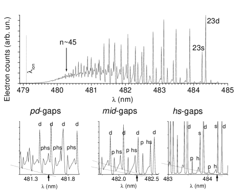
The features of the above type a) develop as follows. As $n$ is increased, the electric field first manifests itself in the appearance of $p$-lines and of triangular-shaped $h$-features (see Fig. 1), caused by electric-field-induced state mixing. Due to the linear Stark effect, the hydrogenic states fan out over an energy range $3n^{2}E$ (atomic units) ([1] and Fig. 2). As $n$ increases further, the $h$-features progressively expand and fill in the spectral gaps of originally zero oscillator strength between the discrete non-hydrogenic $s$-, $p$- and $d$-lines. There are three types of such spectral gaps, which we label $hs$-, $mid$- and $pd$-gaps. The gaps become filled in with significant oscillator strength in exactly that order, at quite well defined critical wavelengths. Those wavelengths can be readily converted into critical effective quantum numbers $n_{\rm hs}$, $n_{\rm mid}$, and $n_{\rm pd}$. The $n_{\rm i}$ are robust indicators for the electric field, because they are solely determined by the general spreading behavior of the quasi-continuous $h$-features. No absolute line strength or line-strength ratio needs to be determined.

Assuming a constant electric field $E_{0}$, the values of $n_{\rm i}$ at which the spectral gaps become filled in can be related to $E_{0}$ using the Stark map of Rb. As shown in Fig. 2, the $hs$-gap below the hydrogenic levels with principal quantum number $n$ disappears when the energy shift of the most red-shifted hydrogenic state, which is approximately $-3n^{2}E_{0}/2$, equals the splitting $0.13n^{-3}$ between the unshifted hydrogenic energy and the next-lower $s$-state. Further, Fig. 2 shows that the $mid$-gaps, i.e. the gaps between the states $(n+3)s$ and $(n+1)d$ and between the field-free hydrogenic states $n-1$ and the states $(n+2)p$, become entirely covered with hydrogenic states at practically identical electric fields. Finally, the $pd$-gaps disappear when neighboring hydrogenic manifolds meet, i.e. when $3n^{2}E_{0}=n^{-3}$. The relations between $E_{0}$ and the critical quantum numbers $n_{\rm i0}$ are obtained as

$$E_{0}= 0.086n_{\rm hs0}^{-5}$$ (1)

$$E_{0}= 0.23n_{\rm mid0}^{-5}$$ (2)

$$E_{0}= 0.33n_{\rm pd0}^{-5}\,{\rm(atomic\,units)}.$$ (3)

The zeros in the subscripts indicate that these relations hold for a constant electric field. Atomic species with quantum defects different from Rb would follow similar relations with different numerical factors. Further, the Eqs. 3 share, as expected, the $n^{-5}$ dependence of the familiar Inglis-Teller relation [11].

 

FIG. 2.: Stark map of Rb in the vicinity of the $n=19$ and $n=20$ hydrogenic manifolds.

To model our experimental spectra, we have calculated the photoabsorption spectra $S(E_{0},\lambda)$ of randomly oriented atoms in constant electric fields $E_{0}$. Since from the $5P$ intermediate state we excite three manifolds of the magnetic quantum number $|m|$, one spectrum $S(E_{0},\lambda)$ is a properly weighted sum of an $m=0$, an $m=1$ and an $m=2$ spectrum. The spectra are obtained as outlined in [12] using a spherical basis set of all states up to $n=90$. To account for the laser linewidth, the spectra are convoluted with Gaussians of a few GHz FWHM. The calculated spectra, one of which is shown in Fig. 3 a), display the same qualitative features as our experimental spectra. This applies, in particular, to the triangular shape of the $h$-features, which is produced by the unresolved excitation of the states in the hydrogenic manifolds.

An investigation of the calculated photoexcitation spectra reveals that the closing of the $pd$-gap appears particularly sudden due to the following peculiarity: for parameters between the $mid$-gap and the $pd$-gap closing, indicated by a double-arrow in Fig. 2, the blue-shifting hydrogenic levels within the $pd$-gap, marked with open circles in Fig. 2, carry much less oscillator strength than all the other nearby hydrogenic levels. As a result, the whole $pd$-gap appears virtually oscillator-strength-free up until the $pd$-gap closing condition $3n^{2}E_{0}\geq n^{-3}$ is satisfied. Once the $pd$-gap closing condition is satisfied, the oscillator strength of the hydrogenic states inside the $pd$-gap increases rather abruptly. This behavior enhances the clarity of the $pd$-gap closing.

 

FIG. 3.: Calculated isotropic excitation spectra of ⁸⁷Rb 5P atoms into Rydberg states. Panel a) is for a homogeneous electric field $E_{0}=6\times 10^{-9}$at. un.$=31$V/cm. Panel b) shows the excitation spectrum - upside down - in a Gaussian cloud of $4\times 10^{5}$ Rb⁺ ions that has a most probable electric field of $E_{\rm max}=31$V/cm. The arrows mark the critical wavelengths where the spectral gaps of low oscillator strength become filled in.

The electric field experienced by the $5P_{3/2}$-atoms is not homogeneous but follows a probability distribution $P(E)$. Assuming identical Gaussian density profiles for the ions and the $5P_{3/2}$-atoms embedded in between them, the distribution $P(E)$ can be calculated by a random placement of ion charges and $5P_{3/2}$-atoms using a radial distribution function $P(r)=4\pi r^{2}(2\pi\sigma^{2})^{-3/2}{\rm exp}(-r^{2}/(2\sigma^{2}))$. The resultant field distributions $P(E)$ have well defined most probable electric fields $E_{\rm max}$, which practically coincide with the singularities of the distributions produced by the corresponding smoothed charge distributions (compare the solid and dotted curves in Fig. 4). The effect of the microfields of the discrete ion charges largely is to smear out the singularities produced by the smoothed charge distributions, adding fields significantly larger than $E_{\rm max}$ to the field distribution. Deviations of the density profiles of the ions and the $5P_{3/2}$-atoms from Gaussians will modify $P(E)$, a dominant peak of $P(E)$. However, a most probable field $E_{\rm max}$ and a microfield-induced tail of fields $E>E_{\rm max}$ will remain.

We have used simulated electric-field distributions $P(E)$ to form averages of the spectra $S(E_{0},\lambda)$ weighted by $P(E)$. As shown in panel b) of Fig. 3, one can still easily obtain critical quantum numbers $n_{\rm hs}$, $n_{\rm mid}$, and $n_{\rm pd}$ at which the respective regions of low oscillator strength disappear. The excitation spectra a) and b) in Fig. 3 are, in fact, quite similar, because the $P(E)$ are clearly dominated by fields near the most probable one. The microfield-induced spread of $P(E)$ from $E_{\rm max}$ towards higher fields causes the spectral gaps with low oscillator strength to become filled in at values of $n$ that are slightly lower than in the case of a homogeneous field $E_{0}=E_{\rm max}$.

 

FIG. 4.: Electric-field distributions $P(E)$ in Gaussian ion clouds with $N=4\times 10^{5}$ and $\sigma=0.2$mm. Solid: Distribution obtained by random placement of discrete ion charges following a Gaussian density distribution. Dotted: Field distribution of the corresponding continuous charge density. Dashed: Holtsmark distribution of the microfields in a neutral plasma with the same ion density as in the center of the above Gaussian ion cloud.

Evaluating a number of spectra as shown in Fig. 3 b), we have determined the relations between the most probable fields $E_{\rm max}$ and the critical effective quantum numbers $n_{\rm hs}$, $n_{\rm mid}$, and $n_{\rm pd}$ for Rydberg atoms excited in Gaussian ion clouds with a FWHM of about 1mm:

$$E_{\rm max}= 0.050n_{\rm hs}^{-5}$$ (4)

$$E_{\rm max}= 0.145n_{\rm mid}^{-5}$$ (5)

$$E_{\rm max}= 0.26n_{\rm pd}^{-5}\,{\rm(atomic\,units)},$$ (6)

We have used Eqs. 6 to experimentally determine the values of $E_{\rm max}$ in ion clouds with diameters of $\sim 1$mm and various ion numbers. The spectra obtained in a few such experiments are displayed in Fig. 5. The critical wavelengths, indicated by arrows, have been determined as shown in Figs. 1 and 3, and have been converted into critical quantum numbers $n_{\rm hs}$, $n_{\rm mid}$ and $n_{\rm pd}$. Using Eq. 6, up to three spectroscopic measurements of $E_{\rm max}$ are obtained for each spectrum. The relative uncertainty of each single electric-field value is $30\%$. Within that uncertainty, the different electric-field values obtained for the individual spectra agree well. The electric field values quoted in Fig. 5 are the averages over all field values obtained for the respective spectra.

The most probable field $E_{\rm max}$ in Gaussian ion clouds can be calculated as $E_{\rm max}=(3.1\times 10^{-10}N_{\rm ion}\sigma^{-2})$Vm, with the RMS cloud size $\sigma$ and ion number $N_{\rm ion}$. We have independently deduced $N_{\rm ion}$ from measurements of the MOT fluorescence. The values of $\sigma$ could be determined from cuts through CCD images of the atom cloud fluorescence, yielding values of $\sigma$ ranging from 0.3mm to 0.5mm. For large atom clouds, we have found that the measured fields exceed the calculated ones by up to a factor of ten. As the atom cloud size is decreased, the discrepancy drops to about a factor of two. The fields deduced from the spectra are, of course, the ones to be trusted. The most likely explanation for the discrepancy and its dependence on the size of the atomic cloud is that the ions were actually not excited in the whole atomic cloud, but were concentrated in a significantly smaller volume determined by the diameters of the excitation laser pulses.

 

FIG. 5.: Experimental excitation spectra of ⁸⁷Rb 5P_3/2 atoms embedded in photo-excited plasmas that contain the indicated numbers $N_{\rm ion}$ of Rb⁺-ions. The $\sigma$-parameters of the utilized Gaussian clouds of laser-cooled atoms are also shown. The most probable electric fields $E_{\rm max}$, shown on the right, are spectroscopically determined and carry an uncertainty of about $20\%$.

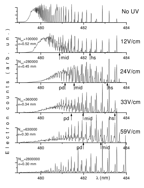
If the number of ions in a Gaussian cloud exceeds $7.8\times 10^{5}{\rm mm}^{-1}\sigma$, the potential depth $U_{0}$ of the ion plasma exceeds $0.9$eV, and a fraction of the UV-excited photoelectrons will be retained [6]. This is clearly the case in the lowest two spectra of Fig. 5, where we exceed the critical ion number by factors $>2.5$ and $>10$, respectively. If the fraction of retained electrons is large, a macroscopically close-to-neutral plasma core is formed, which is surrounded by a positively charged ionic shell. The electric field in the core is close to zero, while the shell carries a large electric field. The distribution $P(E)$ will thus become bi-modal, featuring a peak near $E=0$ and a high-field peak. Rydberg atoms excited in the shell produce the spectroscopic field signatures discussed in this paper, while atoms excited in the core contribute a low-field excitation spectrum with resolved Rydberg resonances up to large $n$. The excitation spectra shown in the two lowest plots of Fig. 5 appear, in fact, as superpositions of a high-field and a low-field spectrum, as expected for bi-modal distributions $P(E)$. In the lowest curve, the high-field component of $P(E)$ apparently is strongly dominated by the low-field one, making it hard to determine the value of the electric field in the shell. The presence of a strong electric field, can, however, be guessed from the appearance of $p$-lines at long wavelengths.

We note that in the case of perfect macroscopic neutrality of the core the microfields in the core would follow a Holtsmark distribution [13], as displayed in Fig. 4. For our charge carrier densities and laser linewidths, the Holtsmark fields are too low to be detectable.

In this work, we have used spectroscopic tools to probe the electric fields in small, laser-excited plasmas. The technique has a large future potential: using crossed and focused Rydberg atom excitation beams, it will be possible to perform spatially resolved measurements of the plasma electric fields. A variation of the time delay between the UV pulse and the blue probe pulse will allow one to study the plasma expansion via the decay of the electric field. The use of a laser with a narrow bandwidth ($\sim 1$MHz) will allow one to detect smaller fields, such as the Holtsmark fields, and to make precise measurements of the detailed electric-field distribution $P(E)$. Measurements of $P(E)$ could reveal inhomogeneities and instabilities in the plasma, which are expected to produce structures in $P(E)$ at excessive fields. Spatial order in the charge carrier arrangement, such as Wigner crystals [14] and the formation of crystalline Rydberg matter [9] may become detectable via measurements of $P(E)$.

Support by NSF is acknowledged. We thank Prof. P. Bucksbaum for inspiring discussions and generous loaning of equipment.

REFERENCES

- [1] T. F. Gallagher, Rydberg Atoms, Cambridge University Press, Cambridge 1994.
- [2] T. W. Ducas, W. P. Spencer, A. G. Vaidyanathan, W. H. Hamilton, D. Kleppner, App. Phys. Lett. 35, 382 (1979), H. Figger, R. Straubinger, H. Walther, G.Leuchs, Opt. Comm. 33, 37 (1980), M. Gross, P. Goy, C. Fabre, S. Haroche, J. M. Raimond, Phys. Rev. Lett. 43, 343 (1979).
- [3] J. Neukammer, H. Rinneberg, K. Vietzke, A. König, H. Hieronymus, M. Kohl, H.-J. Grabka, G. Wunner, Phys. Rev. Lett. 59, 2947 (1987).
- [4] Cavity Quantum Electrodynamics, ed. P. R. Berman (Academic Press, Inc., San Diego 1994).
- [5] B. N. Ganguly, J. Appl. Phys. 6], 571 (1986), J. R. Shoemaker et. al., Appl. Phys. Lett. 52, 2019 (1988), G. A. Hebner et. al., J. Appl. Phys. 76, 4036 (1994).
- [6] T. C. Killian et. al., Phys. Rev. Lett. 83, 4776 (1999).
- [7] Y. Hahn, Phys. Lett. A 231, 82 (1997).
- [8] D. H. E. Dubin, J. P. Schiffer, Phys. Rev. E 53, 5249 (1996).
- [9] E. A. Manykin, M. I. Ozhovan, P. P. Poluektov, Sov. Phys. JETP 57, 256 (1983), L. Homlid, E. A. Manykin, Zh. Eksp. Theor. Fiz. 111, 1601 (1997), R. Svensson, L. Holmlid, Phys. Rev. Lett. 83, 1739 (1999).
- [10] S. Dutta, D. Feldbaum, G. Raithel, submitted and LANL eprint http://xxx.lanl.gov/abs/physics/0003109, (2000).
- [11] D. R. Inglis, E. Teller, J. Astrophys. 90, 439 (1939).
- [12] M. L. Zimmerman, M. G. Littman, M. M. Kash, D. Kleppner, Phys. Rev. A 20, 2551 (1979).
- [13] S. Chandrasekhar, in Selected papers on noise and stochastic processes, ed. N. Wax (Dover, New York 1954).
- [14] S. Ichimaru, Rev. Mod. Phys. 54, 1017 (1982).