Higher Order Force Gradient Symplectic Algorithms

Abstract

We show that a recently discovered fourth order symplectic algorithm, which requires one evaluation of force gradient in addition to three evaluations of the force, when iterated to higher order, yielded algorithms that are far superior to similarly iterated higher order algorithms based on the standard Forest-Ruth algorithm. We gauge the accuracy of each algorithm by comparing the step-size independent error functions associated with energy conservation and the rotation of the Laplace-Runge-Lenz vector when solving a highly eccentric Kepler problem. For orders 6, 8, 10 and 12, the new algorithms are approximately a factor of $10^{3}$, $10^{4}$, $10^{4}$ and $10^{5}$ better.

I Introduction

Symplectic algorithms[1, 2] for solving classical dynamical problems exactly conserve all Poincar$\acute{\rm e}$ invariants. For periodic orbits, the errors in energy conservation are bounded and periodic. This is in sharp contrast to Runge-Kutta type algorithms, whose energy error increases linearly with integration time, even for periodic orbits[3, 4]. Thus, symplectic algorithms are ideal for long time integration of equations of motion in problems of astrophysical interest[5]. For long time integrations, higher order algorithms are desirable because they permit the use of larger time steps. Symplectic algorithms are also advantageous in that higher order algorithms can be systematically generated from any low, even order algorithm[6, 7, 8]. In this work, we will show that higher order algorithms generated by a fourth order force gradient symplectic algorithm[9], have energy errors that are several orders of magnitude smaller than existing symplectic algorithms of the same order. For completeness, we will briefly summarize the operator derivation of symplectic algorithms and their higher order construction in Section II. While the materials in this section are not new, we believe that we have restated Creutz’ and Gockach’s[6] triplet construction of higher order algorithms in its most transparent setting. In sections III and IV we recall force gradient algorithms and discuss two distinct ways of gauging the errors of an algorithm when solving the Kepler problem. We present our results and conclusions in Sections V and VI.

II Operator Factorization and Higher Order Constructions

After a tortuous start[10, 11], symplectic algorithms can be derived most simply on the basis of operator decomposition or factorization. For any dynamical variable $W(q_{i},p_{i})$, its time evolution is given by the Poisson bracket,

$${{d}\over{dt}}W(q_{i},p_{i})=\{W,H\}\equiv\sum_{i}\Bigl{(}{{\partial W}\over{\partial q_{i}}}{{\partial H}\over{\partial p_{i}}}-{{\partial W}\over{\partial p_{i}}}{{\partial H}\over{\partial q_{i}}}\Bigr{)}.$$ (1)

If the Hamiltonian is of the form,

$$H(p,q)={1\over{2}}\sum_{i}p_{i}^{2}+V(\{q_{i}\}),$$ (2)

the evolution equation (1) can be written as an operator equation

$${{dW}\over{dt}}=\sum_{i}\Bigl{(}{p_{i}}{{\partial}\over{\partial q_{i}}}+F_{i}{{\partial}\over{\partial p_{i}}}\Bigr{)}W,$$ (3)

with formal solution

$$W(t)={\rm e}^{t(T+V)}W(0),$$ (4)

where $T$ and $V$ are first order differential operators defined by

$$T\equiv\sum_{i}{p_{i}}{{\partial}\over{\partial q_{i}}},\qquad V\equiv\sum_{i}F_{i}{{\partial}\over{\partial p_{i}}}.$$ (5)

Their exponentiations, ${\rm e}^{\epsilon T}$ and ${\rm e}^{\epsilon V}$, are displacement operators which displace $q_{i}$ and $p_{i}$ forward in time via

$$q_{i}\rightarrow q_{i}+\epsilon{p_{i}}{\hbox{\qquad}}{\rm and}\qquad p_{i}\rightarrow p_{i}+\epsilon F_{i}.$$ (6)

Thus, if ${\rm e}^{\epsilon(T+V)}$ can be factorized into products of the displacement operators ${\rm e}^{\epsilon T}$ and ${\rm e}^{\epsilon V}$, each such factorization gives rise to an algorithm for evolving the system forward in time. For example, the second order factorization

$${\cal T}_{2}(\epsilon)\equiv{\rm e}^{{1\over 2}\epsilon T}{\rm e}^{\epsilon V}{\rm e}^{{1\over 2}\epsilon T}={\rm exp}[\epsilon(T+V)+\epsilon^{3}C++O(\epsilon^{5})\cdots],$$ (7)

corresponds to the second order algorithm

$${\bf q}_{1}= {\bf q}_{0}+{1\over 2}\epsilon{\bf p}_{0},$$ (8)

$${\bf p}_{1}= {\bf p}_{0}+\epsilon{\bf F}({\bf q}_{1}),$$ (9)

$${\bf q}_{2}= {\bf q}_{1}+{1\over 2}\epsilon{\bf p}_{1},$$ (10)

where ${\bf q}_{0}$, ${\bf p}_{0}$ and ${\bf q}_{2}$, ${\bf p}_{1}$ are the initial and final states of the algorithm respectively. This second order symplectic algorithm only requires one evaluation of the force.

The bilaterally symmetric form of ${\cal T}_{2}(\epsilon)$ automatically guarantees that it is time-reversible,

$${\cal T}_{2}(-\epsilon){\cal T}_{2}(\epsilon)=1,$$ (11)

and implies that $\log({\cal T}_{2})$ can only be an odd function of $\epsilon$, as indicated in (7). The explicit form of the operator $C$ is not needed for our present discussion.

Consider now the the symmetric triple product

$${\cal T}_{2}(\delta){\cal T}_{2}(-s\delta){\cal T}_{2}(\delta)={\rm exp}[(2-s)\delta(T+V)+(2-s^{3})\delta^{3}C+O(\delta^{5})+\cdots].$$ (12)

This algorithm evolves the system forward for time $\delta$, backward for time $s\delta$ and forward again for time $\delta$. Since it is manifestly time-reversible, its error terms must be odd powers of $\delta$ only. Morever, its leading first and third order terms can only be the sum of the first and third order terms of each constituent algorithm as indicated. This is because non-additive terms must come from commutators of operators and the lowest order non-vanishing commutator has to have two first order terms and one third order term, which is fifth order. The form of (12) naturally suggests that the third order error term can be made to vanish by choosing

$$s=2\,^{1/3}.$$ (13)

Thus if we now rescale $\delta$ back to the standard step size by setting $\epsilon=(2-s)\delta$, the resulting triplet product would be correct to 4th order,

$${\cal T}_{4}\equiv{\cal T}_{2}\Bigl{(}{\epsilon\over{2-s}}\Bigr{)}{\cal T}_{2}\Bigl{(}{-s\,\epsilon\over{2-s}}\Bigr{)}{\cal T}_{2}\Bigl{(}{\epsilon\over{2-s}}\Bigr{)}={\rm exp}[\,\epsilon(T+V)+O(\epsilon^{5})+\cdots].$$ (14)

Expanding out the ${\cal T}_{2}\,$’s gives the explicit form:

$${\cal T}_{4}\equiv{\rm e}^{a_{1}\epsilon T}{\rm e}^{b_{1}\epsilon V}{\rm e}^{a_{2}\epsilon T}{\rm e}^{b_{2}\epsilon V}{\rm e}^{a_{2}\epsilon T}{\rm e}^{b_{1}\epsilon V}{\rm e}^{a_{1}\epsilon T}$$ (15)

where, by inspection

$$a_{1}={1\over 2}{1\over{2-s}},\quad a_{2}=-{1\over 2}{{s-1}\over{2-s}},\quad b_{1}={1\over{2-s}},\quad{\rm and}\quad b_{2}=-{s\over{2-s}}.$$ (16)

This fourth order symplectic algorithm was apparently obtained by E. Forest in 1987. However, its original derivation was very complicated and was not published with Ruth[11] until 1990. During this period many groups, including Campostrini and Rossi[12] in 1990, Candy and Rozmous[13] in 1991, independently published the same algorithm. Our discussion followed the earliest published derivation of this algorithm by Creutz and Gocksch[6] in 1989. After they were informed of this algorithm by Campostrini, they provided the triplet construction and generalized it to higher order. The triplet construction was also independently published by Suzuki[7] and Yoshida[8] in 1990.

Higher order algorithms can be obtained by repeating this construction. Starting with any $n$th order symmetric algorithm,

$${\cal T}_{n}(\epsilon)={\rm exp}[\,\epsilon(T+V)+\epsilon^{(n+1)}D+\cdots],$$ (17)

the triplet product

$${\cal T}_{n}(\delta){\cal T}_{n}(-s\delta){\cal T}_{n}(\delta)={\rm exp}[(2-s)\delta(T+V)+(2-s^{n+1})\delta^{n+1}D+O(\delta^{n+3})+\cdots],$$ (18)

will be of order $(n+2)$ if we choose

$$s=2\,^{1/(n+1)}$$ (19)

and renormalize $\delta=\epsilon/(2-s)$ as before.

III Force Gradient Algorithms

The method of operator factorization can be applied to many different classes of evolution equations. However, the triplet concatenations with a negative time step are a special construction with more limited applicability. For example, one cannot use it to derive similar Diffusion Monte Carlo or finite temperature path integral algorithms, because one cannot simulate diffusion backward in time nor sample configurations with negative temperatures. The triplet construction is a special example of Suzuki’s[14] general proof that, beyond second order, it is impossible to factorize ${\rm e}^{\epsilon(T+V)}$ only into products of ${\rm e}^{\epsilon T}\,$’s and ${\rm e}^{\epsilon V}\,$’s without introducing negative time steps. For symplectic algorithms this means that one can never develop a purely positive time step fourth order algorithm by evaluating only the force. For many years the Forest-Ruth (FR) algorithm was the only known fourth order symplectic algorithm. Recently, a deeper understanding of the operator factorization process has yielded three new symplectic algorithms[9] all with purely positive time steps. These new algorithms circumvented Suzuki’s no-go theorem by evaluating the force and its gradient. This corresponds to factorizing ${\rm e}^{\epsilon(T+V)}$ in terms of operators $T$, $V$, and the commutator $[V,[T,V]]$. The latter corresponds to

$$[V,[T,V]]=2F_{j}{{\partial F_{i}}\over{\partial q_{j}}}{{\partial}\over{\partial p_{i}}}=\nabla_{i}|{\bf F}|^{2}{{\partial}\over{\partial p_{i}}},$$ (20)

which is the gradient of the squared magnitude of the force. Of the three algorithms derived by Chin[9], algorithm C is particularly outstanding and corresponds to the factorization

$${\rm e}^{\epsilon(T+V)}={\rm e}^{\epsilon{1\over 6}T}{\rm e}^{\epsilon{3\over 8}V}{\rm e}^{\epsilon{1\over 3}T}{\rm e}^{\epsilon{1\over 4}\widetilde{V}}{\rm e}^{\epsilon{1\over 3}T}{\rm e}^{\epsilon{3\over 8}V}{\rm e}^{\epsilon{1\over 6}T}+O(\epsilon^{5}).$$ (21)

where

$$\widetilde{V}=V+{1\over 48}\epsilon^{2}[V,[T,V]].$$ (22)

The algorithm itself can be read off directly as

$${\bf q}_{1} ={\bf q}_{0}+{1\over 6}\epsilon{\bf p}_{0},$$ (23)

$${\bf p}_{1} ={\bf p}_{0}+{3\over 8}\epsilon{\bf F}({\bf q}_{1})$$ (24)

$${\bf q}_{2} ={\bf q}_{1}+{1\over 3}\epsilon{\bf p}_{1}$$ (25)

$${\bf p}_{2} ={\bf p}_{1}+{1\over 4}\epsilon\Bigl{[}{\bf F}({\bf q}_{2})+{1\over{48}}\epsilon^{2}\nabla|{\bf F}({\bf q}_{2})|^{2}\Bigr{]}$$ (26)

$${\bf q}_{3} ={\bf q}_{2}+{1\over 3}\epsilon{\bf p}_{2}$$ (27)

$${\bf p}_{3} ={\bf p}_{2}+{3\over 8}\epsilon{\bf F}({\bf q}_{3})$$ (28)

$${\bf q}_{4} ={\bf q}_{3}+{1\over 6}\epsilon{\bf p}_{3}.$$ (29)

In [9] it was shown that the maximum energy error for this algorithm, when used to solve Kepler’s problem, is smaller than that of the FR algorithm by a factor of 80. At the moment there is no general method for constructing higher order algorithms with only positive time steps. It is not even known whether a positive time step 6th order algorithm exists. Thus, beyond 4th order the triplet contruction is still the only systematic way of generating higher order algorithms. In this work we show that intrinsic error functions associated with higher order algorithms generated from Chin’s algorithm C are far smaller than those generated from the FR algorithm.

IV The Energy and the LRL Vector

We gauge the numerical effectiveness of each algorithm by solving the two dimensional Kepler problem

$${{d^{2}{\bf q}}\over{dt^{2}}}=-{{\bf q}\over{q^{3}}},$$ (30)

with initial conditions ${\bf q}_{0}=(10,0)$ and ${\bf p}_{0}=(0,1/10)$. The resulting highly eccentric (e=0.9) orbit provides a non-trivial testing ground for trajectory integration.

A symmetric $n$th order symplectic algorithm evolves this system forward in time with Hamiltonian

$$H({\bf p},{\bf q})=H_{0}({\bf p},{\bf q})+\epsilon^{n}H_{n}({\bf p},{\bf q})+O(\epsilon^{n+2}),$$ (31)

which deviates from the exact Hamiltonian $H_{0}({\bf p},{\bf q})={1\over 2}{\bf p}^{2}-1/|{\bf q}|$ by an error term $\epsilon^{n}H_{n}({\bf p},{\bf q})$ as indicated. To gauge the intrinsic merit of each algorithm we compare their step-size independent error coefficient $H_{n}({\bf p},{\bf q})$. This can be extracted numerically as follows. Let’s start the system with total energy $E_{0}=H_{0}({\bf p}(0),{\bf q}(0))$. Since the Hamiltonian (31) is conserved by the algorithm, we have

$$E_{0}=H_{0}({\bf p}(t),{\bf q}(t))+\epsilon^{n}H_{n}({\bf p}(t),{\bf q}(t))+O(\epsilon^{n+2})$$ (32)

Denoting $E(t)\equiv H_{0}({\bf p}(t),{\bf q}(t))$ and $H_{n}(t)=H_{n}({\bf p}(t),{\bf q}(t))$, we therefore have

$$H_{n}(t)=-\lim_{\epsilon\rightarrow 0}{1\over{\epsilon^{n}}}\Bigl{[}E(t)-E_{0}\Bigr{]}.$$ (33)

Energy conservation does not directly measure how well the orbit is determined. When the time step is not too small, a very noticeable error is that the orbit precesses. One can, but it is tedious, directly monitor this orbital precession[4]. It is more expedient to follow the rotation of the Laplace-Runge-Lenz (LRL) vector:

$${\bf A}={\bf p}\times{\bf L}-\hat{\bf r}.$$ (34)

When the orbit is exact the LRL vector is constant, pointing along the semi-major axis of the orbit. When the orbit precesses the LRL vector rotates correspondingly.

For an $n$th order algorithm,

$${{d{\bf A}}\over{dt}}=\epsilon^{n}\sum_{i}\Bigl{(}{{\partial{\bf A}}\over{\partial q_{i}}}{{\partial H_{n}}\over{\partial p_{i}}}-{{\partial{\bf A}}\over{\partial p_{i}}}{{\partial H_{n}}\over{\partial q_{i}}}\Bigr{)}.$$ (35)

Thus, the rate of change of each component of the LRL vector is of order $\epsilon^{n}$. The components themselves, which are time integrals of the above modulo a constant term, must also be of order $\epsilon^{n}$. Let the LRL vector initially be of length ${A_{0}}$ and lie along the x-axis, then we have

$$A_{x}(t) =A_{0}+\epsilon^{n}A_{nx}(t)+O(\epsilon^{n+2}),$$ (36)

$$A_{y}(t) =\epsilon^{n}A_{ny}(t)+O(\epsilon^{n+2}).$$ (37)

Since the square of the LRL vector is related to the energy by

$${\bf A}^{2}=2{\bf L}^{2}E+1,$$ (38)

the longitudinal deviation coefficient $A_{nx}(t)$ is related to the energy error coefficient by

$$A_{nx}(t)={1\over{\epsilon^{n}}}{{\bf L}^{2}\over{A_{0}}}(E(t)-E_{0})=-{{\bf L}^{2}\over{A_{0}}}H_{n}(t),$$ (39)

which gives no new information. The perpendicular deviation coefficient $A_{ny}(t)$ is best measured in terms of the rotation angle:

$$\theta(t)=\tan^{-1}\biggl{[}{{A_{y}(t)}\over{A_{x}(t)}}\biggr{]}=\epsilon^{n}\biggl{[}{{A_{ny}(t)}\over{A_{0}}}\biggr{]}+\cdots$$ (40)

To compare algorithms we again extract and compare their rotation error coefficient function $\theta_{n}(t)=A_{ny}(t)/A_{0}$ via

$$\theta_{n}(t)=\lim_{\epsilon\rightarrow 0}{1\over{\epsilon^{n}}}\theta(t).$$ (41)

Since this rotational angle is related to some integral of the energy error function, it is a better measure of the overall error of the algorithm.

V Results of Comparing Higher Order Algorithms

By use of the triplet construction, we generated 6th, 8th, 10th, and 12th order algorithms from both the Forest-Ruth and Chin’s C algorithm. We computed the fractional energy deviation, which is just the negative of the energy error coefficient normalized by the initial energy,

$$\lim_{\epsilon\rightarrow 0}{1\over{\epsilon^{n}}}\Bigl{[}{{E(t)}\over{E_{0}}}-1\Bigr{]}=-{{H_{n}(t)}\over{E_{0}}}.$$ (42)

Smaller and smaller time steps $\epsilon$ are used until the extracted coefficient function is stablized independent of the time step size. This typically occurs in the neighborhood of $\epsilon=P/5000$, where P is the period of the orbit.

Fig.1 compares the (negative) normalized error coefficient functions for the 4th order Runge-Kutta, Forest-Ruth and Chin’s C algorithms over one period of the orbit. The error function for the two symplectic algorithms are substantial only near mid period when the particle is at its closest approach to the attractive center. For symplectic algorithms energy is conserved over one period, or its non-conservation is periodic. Its average energy error is bounded and constant as a function of time. In contrast, the 4th order Runge-Kutta energy error function is an irreversible, step-like function over one period. Each successive period will increase the error by the same amount resulting in a linearly rising, staircase-like error function in time. As noted earlier, the maximum error in Chin’s algorithm C is smaller than that of the FR algorithm by a factor of 80. However, this error height comparison at one point is not meaningful. It is better to compare the energy error averaged over one period. This would require the integral of the energy error function. On this basis algorithm C will be better still. While the energy error integral can be done, the same goal can be achieved by monitoring the rotation of the LRL vector.

Fig.2 shows the corresponding error coefficient functions of the rotational angle of the LRL vector. After each period, the algorithms rotate the LRL vector by a definite amount. The error coefficient provides an intrinsic, step-size independent way of comparing this rotation. In Fig.2 the rotated angle produced by algorithm C is too small to be visible when plotted on the same scale as the other algorithms. The insert gives an enlargement of the details. The rotational angle of the LRL vector appears to be related to some integral of energy error function. Although we have not been able to demonstrate this analytically, numerical integration of the energy error function does give a function similiar in shape to the angle coefficient function, having the same numbers of maxima and minima. For the Runge-Kutta, Forest-Ruth and Chin’s C 4th order algorithms, the magnitudes of this rotation cofficient after one period are 2.666, 10.860, and 0.004 respectively. On this basis, algorithm C is better than FR by a factor of $\approx 3000$. When the orbit is integrated over many periods the rotational angle from symplectic algorithms increases linearly in a staircase-like manner with time. In contrast, the rotational angle of the Runge-Kutta algorithm shows a quadratic increase over long times, such as a few thousand periods. This result is easy to understand if the rotational angle is related to some integral of the energy error. This quadratic increase in the rotation angle of the LRL vector clearly mirrors the quadratic increase in phase error of the Runge-Kutta algorithm, as discussed by Gladman, Duncan and Candy[4].

Fig.3 and Fig.4 show the results when both the Forest-Ruth and Chin’s C algorithms are iterated to 6th order by the triplet product construction. Inserts in both detail algorithm C’s intricate structure. As an added comparison we also included results for Yoshida’s[8] 6th order algorithm A, which is a product of 7 second order algorithms (10), some with negative time steps. For Yoshida’s algorithm, Forest-Ruth and Chin’s C algorithm in 6th order, the magnitudes of the rotation cofficients after one period are 11.44, 335.1, and 0.1156 respectively. Yoshida’s algorithm is a factor of 30 better than FR, but algorithm C is a factor of 3000 better. Note that if the energy error function is related to the differential of the the angle error function, the zeros of the former would correspond to the extrema of the latter. The four zero crossings of algorithm C’s energy error function are clearly reflected in the two maxima and two minima of the corresponding angle error function.

Fig.5 and Fig.6 give results for the 8th order iterated algorithms based on the Forest-Ruth and Chin’s C algorithm. The magnitudes of the angle error coefficients are $1.386\times 10^{4}$ and 0.4532 respectively, giving a ratio of approximately $3\times 10^{4}$. Algorithm C retains its characteristic shape in both the energy and the angle error function. Fig.7 and Fig.8 give the corresponding results for the iterated 10th order algorithms. Here the intricate structure in the C algorithm is beginning to be washed out. At this high order, quadruple numeric precision is necessary to extract these coefficient functions smoothly. The magnitudes of the angle error coefficients are now $7.141\times 10^{5}$ and $17.89$ respectively, giving a ratio of $4\times 10^{4}$. Fig.9 and Fig.10 give similar results for the 12th order algorithms. At this point all structures in the C algorithm are gone. The magnitudes of the angle error coefficients are now $4.473\times 10^{7}$ and $427.5$ respectively, giving a ratio of $1.05\times 10^{5}$.

The iteration of algorithms A and B of Chin[9] also produced results that are better than FR based algorithms. However, we do not detail their results here because they are at least one or two orders of magnitude inferior to algorithm C.

VI Conculsions

In this work we have shown that higher order force gradient symplectic algorithms appear to be superior to non-gradient symplectic alogorithms as measured by eneregy conservation and the rotation of the LRL vector. While it has been shown earlier that 4th order force gradient algorithms have smaller energy error coefficients[9], it was not known that this advantage would mulitply dramatically when algorithms are iterated to higher orders. The conclusion that one should draw may not be that force gradient algorithms are better, but that higher order non-gradient algorithms are far from optimal. Secondly, we suggested that the rotation of the LRL vector gives an intergrated measure of an algorithm’s merit when tested on the Kepler problem.

The high accuracy of this class of algorithms seemed ideal for long time integration of few-body problems, such as that of the solar system[5]. For such few-body problems, the evaluation of the force gradient is not excessively difficult. It would be useful to examine the merit of this class of algorithms in more physical applications. The distinct advantage uncovered in this work, that it is better to iterate a 4th order algorithm with all positive time steps, gives further impetus to search for an all positive time step 6th order symplectic algorithm.

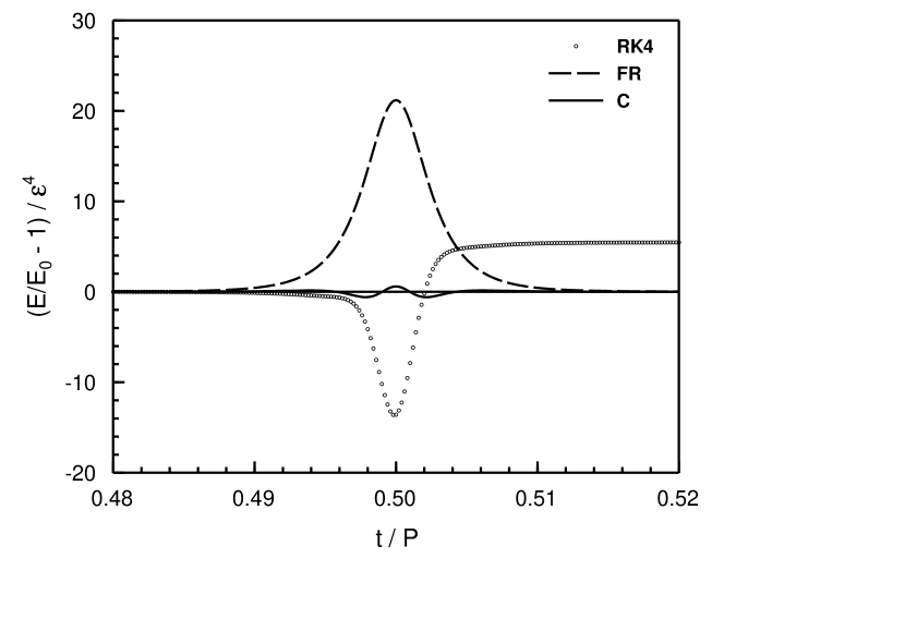
FIG. 1.: The normalized energy deviation of a particle in a Keplerian orbit, which measures the step-size independent energy error coefficient $-H_{4}({\bf p}(t),{\bf q}(t))/E_{0}$. P is the period of the elliptical orbit and $\epsilon$ is the time step size. RK4, FR, and C denote results for the 4th order Runge-Kutta, Forest-Ruth, and Chin’s C algorithm respectively. The maximum deviations for algorithm FR and C are 21 and 0.27 respectively.

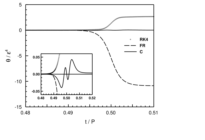
FIG. 2.: The step-size independent error coefficient of the rotation angle of the Laplace-Runge-Lenz vector for 4th order algorithms. The LRL vector rotates substantial only when the particle is near mid period, closest to the attractive center. The insert make visible the fine structure produced by algorithm C.

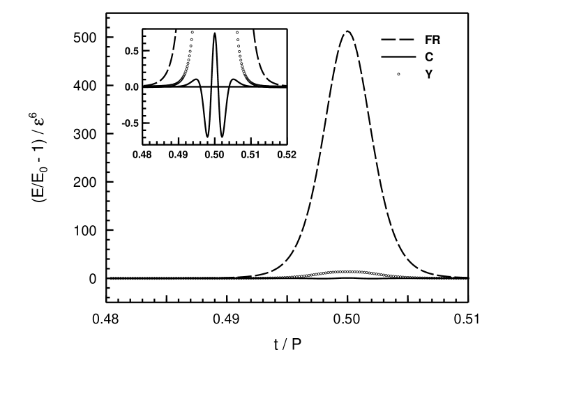
FIG. 3.: The normalized energy deviation for 6th order algorithms. RF and C denote 6th order algorithms generated by a triplet product of corresponding 4th algorithms in Fig.1. The insert makes visible the energy devivation of algorithm C, which is not visible in the bigger graph. The maximum deviations for algorithms FR, Y and C are 513, 13.6, and 0.74 respectively.

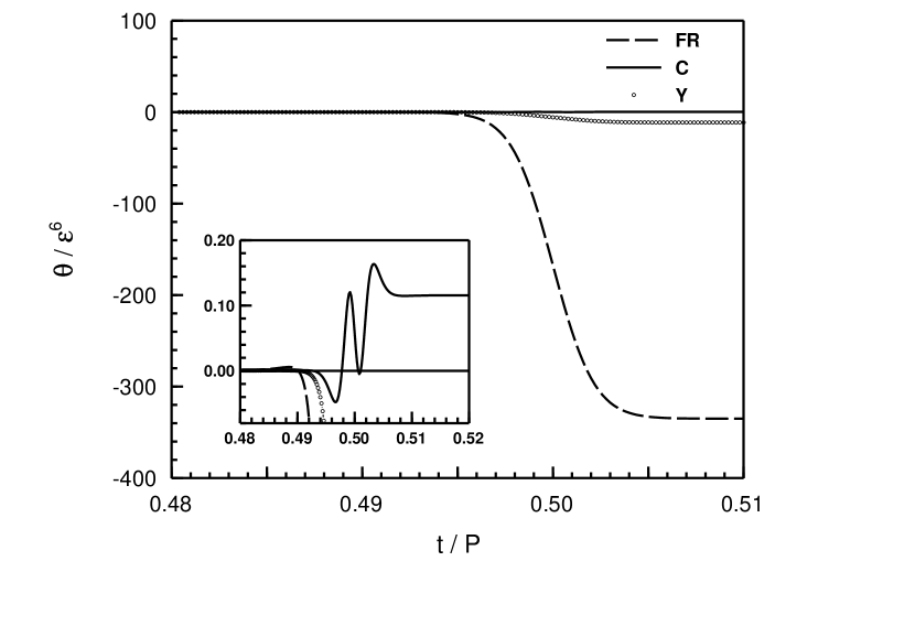
FIG. 4.: The step-size independent error coefficient of the rotation angle of the LRL vector for 6th order algorithms as described in Fig.3. The insert makes visible the minute rotation coefficient produced by algorithm C.

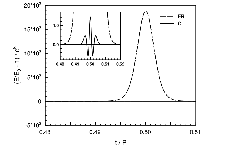
FIG. 5.: The normalized energy deviations for 8th order algorithms, as generated by a triplet product of 6th order algorithm described in Fig.3. The insert makes visible the minute energy deviation of algorithm C.

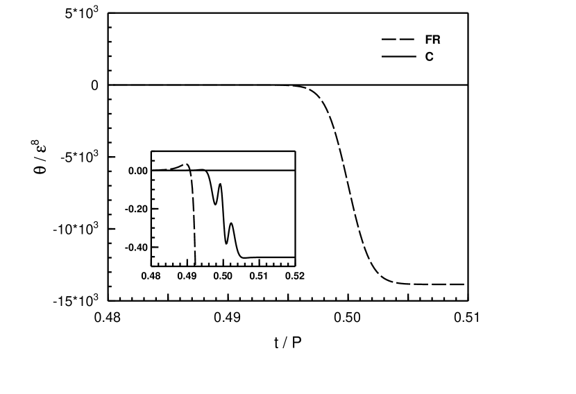
FIG. 6.: The step-size independent error coefficient of the rotation angle of the LRL vector for 8th order algorithms as described in Fig.5. In this order, the algorithm C based algorithm begins to rotate in the same sense as the FR base algorithm.

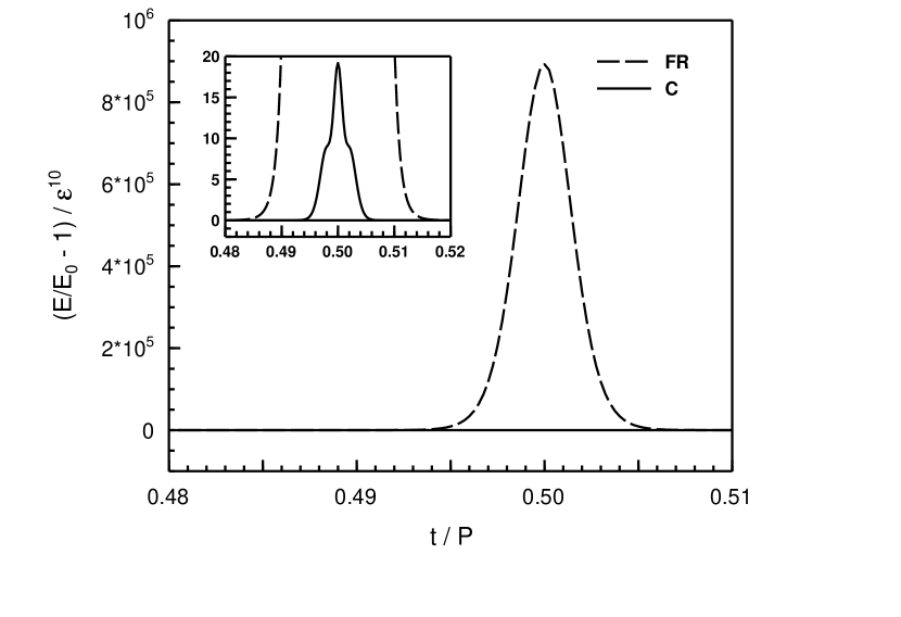
FIG. 7.: The normalized energy deviations for 10th order algorithms, as generated by a triplet product of 8th order algorithm described in Fig.5. The insert shows that the characteristic oscillations of algorithm C are beginning to disappear.

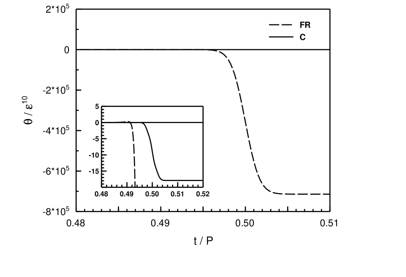
FIG. 8.: The step-size independent error coefficient of the rotation angle of the LRL vector for 10th order algorithms as described in Fig.7. The insert shows that the error coefficient of algorithm C begins to look like that of the FR algorithm.

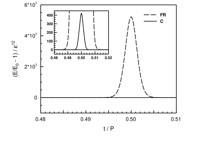
FIG. 9.: The normalized energy deviations for 12th order algorithms, as generated by a triplet product of 10th order algorithm described in Fig.7. The insert shows that there is no longer any distinctive structure produced by algorithm C.

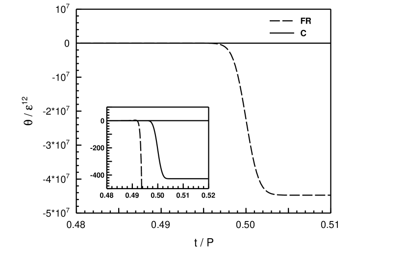
FIG. 10.: The step-size independent error coefficient of the rotation angle of the LRL vector for 12th order algorithms as described in Fig.9. The insert shows that both algorithms have converged to a similar step-like error function.

- [1] Numerical Hamiltonian Problems by J. Sanz-Serna and M. Calvo, Chapman & Hall London, 1994.
- [2] H. Yoshida, Celest. Mech. 56 (1993) 27.
- [3] H. Kinoshita, H. Yoshida, an dH. Nakai, Celest. Mech. 50(1991)59-71.
- [4] B. Gladman, M. Duncan and J. Candy, Celest. Mech. 52(1991)221.
- [5] J. Wisdom and M. Holman, Astrophys. J., 102(1991)1528.
- [6] M. Creutz and A. Gocksch, Phys. Rev. Letts. 63(1989) 9.
- [7] M. Suzuki, Phys. Lett. A146 (1990)319.
- [8] H. Yoshida, Phys. Lett. A150 (1990)262.
- [9] S. A. Chin, Phys. Lett. A226 (1997) 344.
- [10] R. D. Ruth, IEEE Trans. Nucl. Sci, NS-30(1983)2669.
- [11] E. Forest and R. D. Ruth, Physica D 43(1990) 105.
- [12] M. Campostrini and P. Rossi, Nucl. Phys. B329(1990) 753.
- [13] J. Candy and W. Rozmus, J. Comp. Phys. 92(1991) 230.
- [14] M. Suzuki, J. Math. Phys. 32 (1991)400.