Theory of coherent photoassociation of a Bose-Einstein condensate

Abstract

We study coherent photoassociation, phenomena analogous to coherent optical transients in few-level systems, which may take place in photoassociation of an atomic Bose-Einstein condensate but not in a nondegenerate gas. We develop a second-quantized Hamiltonian to describe photoassociation, and apply the Hamiltonian both in the momentum representation and in the position representation (field theory). Solution of the two-mode problem including only one mode each for the atomic and molecular condensates displays analogs of Rabi oscillations and rapid adiabatic passage. A classical version of the field theory for atoms and molecules is used to demonstrate that, in the presence of photoassociating light, a joint-atom molecule is unstable against growth of density fluctuations. Experimental complications, including spontaneous emission and unwanted “rogue” photodissociation from a photoassociated molecule are analyzed. A two-color Raman scheme is studied as a method to set up an effective two-mode scheme with reduced spontaneous emission losses. We discuss photoassociation rates and photoassociation Rabi frequencies for high-lying vibrational states in alkalis both on the basis of molecular-structure calculations, and by comparing with an experiment [Wynar et al., Science 287, 1016 (2000)].

I Introduction

Laser cooling and its spin-offs now routinely produce gaseous samples in which thermal energies, when expressed as frequencies, are smaller than the typical linewidth of an optical dipole transition. Photoassociating transitions, in which two thermal atoms combine in the presence of light to make a molecule, may therefore exhibit linewidths every bit as narrow as the transitions one encounters in nonlinear laser spectroscopy. As a result, photoassociation spectroscopy PATHEO has become the source of the most accurate molecular structure data available. Bose-Einstein condensation BEC is another recent triumph in the quest toward low temperatures in atomic physics. The connection between photoassociation and Bose-Einstein condensation has long been close, though somewhat incidental; photoassociation spectroscopy has provided key numerical data for condensation experiments SCALEN .

There have been early discussions of photoassociation of a condensate itself BUR97 ; JUL98 . However, to us, the true scope of the connection between photoassociation and condensation was only revealed by our explicit observation JAV98 that in a thermal gas it is the same phase space density that governs both the onset of Bose-Einstein condensation and the efficiency of photoassociation.

At the heart of our photoassociation work lies the quasicontinuum (QC) approach JAV98 ; MAC99 . The idea is to enclose two colliding atoms in a box, which has the effect of discretizing the dissociation continuum of the corresponding diatomic molecule. At the end of the calculations, the quantization volume is taken to infinity. Aside from resolving certain mathematical difficulties, this method turns out to have the unexpected benefit that analysis of photoassociation is reverted to analysis of few-level systems, as in quantum optics or laser spectroscopy. For instance, studies of two-color photoassociation schemes may draw from decades of experience in quantum optics and laser spectroscopy MAC99 .

However, in its initial form our QC approach does not apply to a quantum degenerate sample. We sought to rectify this shortcoming by introducing a phenomenological second-quantized Hamiltonian for photoassociation JAV99 . This idea was developed at the same time independently by Drummond et al. DRU98 , and mathematically closely related approaches to the Feshbach resonance are also under active study TIM98 ; TIM99 ; ABE99 . Comparison with the QC approach gives the transition matrix elements to insert into our Hamiltonian.

We first considered a two-mode model that only takes into account one C.M. wave function for atoms and one for molecules, the modes containing the atomic and molecular condensates JAV99 . The main finding was coherent photoassociation analogous to coherent transients in few-level systems. For instance, the system may exhibit a form of Rabi flopping between atoms and molecules. Moreover, by properly sweeping the frequency of the photoassociating laser, in a process akin to rapid adiabatic passage the atomic condensate may be turned into a molecular condensate JAV99 . In another development in this direction, we have argued that two-color free-bound-bound stimulated Raman adiabatic passage, STIRAP, is feasible starting from an atomic condensate MAC00 . We have also gone beyond the two- and three-mode approximations, allowing for an arbitrary position dependence of the atomic and molecular condensates, albeit in a classical approximation similar to the one underlying the Gross-Pitaevskii equation JAV99a . It then turns out that an equilibrium with both atomic and molecular condensates present together with the photoassociating light is unstable. The sample tends to collapse spontaneously into clumps whose densities increase with time JAV99a .

The primary purposes of the present paper are to document the numerous technical and physical details of our second-quantized approach to photoassociation that could not be accommodated by the letter format of Refs. JAV99 , MAC00 , and JAV99a , and to extend our discussion in several directions that support those references. To offer a comprehensive account of the field theory version of our approach to coherent photoassociation, we have found it necessary to analyze the dipole matrix element for photoassociation in detail. This endeavor in effect constitutes an alternative derivation (c.f. Ref. MAC99 ) of our entire QC methodology. Second, we add an analysis of two-color photoassociation of a quantum-degenerate sample in a three-mode approximation that is to some extent complementary to the one in Ref. MAC00 . Much as expected, the two-color scheme provides a reprieve from spontaneous-emission losses from the primary photoassociated state. Third, we present a quantitative analysis of “rogue” photodissociation from a molecular condensate to atomic modes outside the condensate. Our suggestion JAV99 that with increasing light intensity the unwanted photodissociation may overtake coherent condensate-condensate transitions is corroborated. We find a minimum usable time scale proportional to the the inverse of the recoil frequency of laser cooling.

Probably the most prominent qualitative finding emerging from our work is the observation that it is Bose enhancement that ultimately facilitates coherent transients such as Rabi flopping, adiabatic following, and STIRAP in photoassociation of a condensate MAC00 ; MAC00a . Throughout this paper, we continue to demonstrate how coherent optical transients come about in a condensate, and argue why they should be absent in a nondegenerate gas.

There has recently been a remarkable experiment on two-color photoassociation of a condensate WYN00 . Accordingly, we include a detailed discussions on the values of experimental parameters in alkalis in general, and the parameters of Ref.  WYN00 in particular. The analysis of the actual experiment demonstrates that there is still some way to go before genuinely coherent photoassociation is reached.

In Sec. II we give a walk-through of our second-quantized Hamiltonian, including a detailed discussion of the dipole moment matrix element and both the momentum and position representation of the Hamiltonian. The special case with only one spatial mode for both atoms and molecules is the subject of Sec. III. The classical version of the field theory, but including all spatial modes, is the subject of Sec. IV. The numerous complications to our one color scheme that one is liable to encounter in real experiments, as well as the experimental parameter values, are the subject of Sec. V. The brief remarks in Sec. VI conclude the paper. There are also two appendices, A on the details of the relation of the dipole matrix element between second-quantized and quasicontinuum approaches, and B on the role of atom-atom collisions in our development.

II Field theory for atoms and molecules

The task of the present section is to develop in detail the second-quantized approach governing photoassociation of atoms into molecules in the prototype case of one laser color only. Simple heuristic arguments based on Refs. JAV98 ; MAC99 could, and did, achieve most of our aims in Ref. JAV99 where we dealt primarily with the momentum representation, but the field theory of Ref. JAV99a calls for a few additional angles. To support them, we present here a partially new ab-initio discussion of our QC method.

We take the photoassociating atoms to be in precisely one internal state, and similarly we assume that photoassociation leads to molecules with precisely one internal state. These assumptions could be relaxed, but then one has to follow the fate of the internal states as well. We do not go into this, but in essence assume that (i) the atoms are polarized and that (ii) the photoassociation resonance in itself selects a unique final state for the molecule.

II.1 Two atoms

We begin with a pair of atoms, assumedly in the dissociation continuum of a given potential energy curve of a diatomic molecule. As the atoms interact, their relative momentum need not be a constant of the motion. Nonetheless, given a finite range for atom-atom interactions, in free space the wave functions of the relative motion $\phi_{\bf k}({\bf r})$ could still be characterized by the asymptotic ($r\rightarrow\infty$) wave vector ${\bf k}$.

On the other hand, in the spirit of the QC method JAV98 ; MAC99 , we assume that the relative motion of the atoms is confined to a finite volume $V$. There are two basic questions in our two-atom analysis that must be considered. First, our phenomenological many-particle Hamiltonian (Ref. JAV99 and Eq. (12) below) is written down in terms of plane waves, yet it is more common to analyze photoassociation in terms of angular-momentum partial waves. How do we make the connection? Second, in our quasicontinuum method we resort to a finite quantization volume $V$, which tends to infinity only at the end of the calculations. How should we handle the finite quantization volume?

We quantize the relative motion of the two atoms in a spherical box of radius $R$ and volume $V={4\over 3}\pi R^{3}$ using reflecting boundary conditions. While angular momentum is still a constant of the motion, the usual eigenstates MAC99 of the relative motion cannot be characterized by a momentum vector, even asymptotically. Nonetheless, it is evidently possible to construct orthonormal superpositions $\bar{\phi}_{\bf k}({\bf r})$ of the eigenstates of the spherical box that in the limit of a large box turn into the states $\phi_{\bf k}({\bf r})$, i.e., states that behave like plane waves at large distances.

Let us first take the inner product of a true plane wave, normalized to the volume $V$, with a spherically symmetric (real) test function $f(r)$ with a finite range $\ll R$. In the limit ${\bf k}\rightarrow 0$ we have

$$I_{1}=\lim_{{\bf k}\rightarrow 0}\,{1\over\sqrt{V}}\int_{0}^{R}d^{3}r\,e^{i{\bf k}\cdot{\bf r}}f(r)\simeq{1\over\sqrt{V}}\int_{0}^{\infty}4\pi r^{2}\,dr\,f(r)\,.$$ (1)

Next we take the same inner product for the $l=0$ partial wave of the plane wave $e^{i{\bf k}\cdot{\bf r}}$, basically the spherical Bessel function $j_{0}(kr)\propto\sin kr/r$. We normalize this partial wave also in the spherical box, or equivalently, in the radial coordinate $r$ with respect to the measure $4\pi r^{2}\,dr$. In the limit of small $k$ we have the integral for the inner product

$$I_{2} = {1\over\sqrt{2\pi R}}\int_{0}^{R}4\pi r^{2}\,dr\,{\sin kr\over r}f(r)$$ (2)

$$\simeq {k\over\sqrt{2\pi R}}\int_{0}^{\infty}4\pi r^{2}\,dr\,f(r)\,.$$

Obviously, the ratio of the two,

$$\alpha(k)={I_{1}\over I_{2}}={1\over k}{\sqrt{2\pi R\over V}}\,,$$ (3)

is the expansion coefficient of the $s$-wave in the plane wave, given that both the plane wave and the $s$-wave are normalized to the volume $V$. Actually, the $k$ values of the spherical eigenmodes are quantized, and the smallest value is $k=\pi/R$. We therefore have to be careful with the limit $k\rightarrow 0$ when applying Eq. (3).

When atom-atom interactions are taken into account, the radial eigenstates for a given angular momentum are not just spherical Bessel functions, but also reflect the scattering phase shifts. Henceforth we assume that only $s$-wave scattering needs to be considered, as is usually the case for bosons at sufficiently low temperatures. Obviously, even though the partial waves have phase shifts, by tweaking the phases of the partial waves it is still possible to make an asymptotic near-plane wave $\bar{\phi}_{k}({\bf r})$ out of the eigenstates of the relative motion of the atoms in the sphere. The adjustment of phases has no effect on the weight of the $s$-wave component in $\bar{\phi}_{k}({\bf r})$, which may still be inferred from Eq. (3).

Let us denote the wave function of the particular molecular state we are aiming for by $\bar{\psi}({\bf r})$, and make the standard (albeit crude) approximation that the relevant electronic dipole matrix element ${\bf d}$ is a constant independent of the relative coordinate ${\bf r}$ of the atoms comprising the molecule. Then the QC dipole matrix element for photoassociation and photodissociation characterizing a process in which the relative momentum of the colliding atoms is $\hbar{\bf k}$ reads simply

$${\bf d}({\bf k})={\bf d}\int d^{3}r\,\bar{\psi}^{*}({\bf r})\bar{\phi}_{\bf k}({\bf r})\,.$$ (4)

We only consider $s$-wave collisions, and correspondingly set $\bar{\psi}({\bf r})=\bar{\psi}(r)$ as appropriate for a nonrotating $J=0$ molecule. Of course, only the $l=0$ component of the wave function $\bar{\phi}_{\bf k}({\bf r})$ counts. Taking into account the weight from Eq. (3), we have

$${\bf d}({\bf k})={\bf d}\,{1\over k}{\sqrt{2\pi R\over V}}\int_{0}^{R}4\pi r^{2}\,dr\,\bar{\psi}^{*}(r)\bar{\phi}_{k}^{0}(r)\,.$$ (5)

The notation $\bar{\phi}^{0}_{k}(r)$ stands for the radial $l=0$ wave function of the relative motion of the two atoms corresponding to the wave number $k$, and normalized to volume $V$ as usual.

A convenient qualitative model is provided by the limiting form

$$\bar{\phi}^{0}_{k}(r)={1\over\sqrt{2\pi R}}\,{\sin\,k(r-a)\over r}\,,$$ (6)

where $a$ is the $s$-wave scattering length. Combination of (5) and (6) gives

$${\bf d}({\bf k})={\bf d}\,{4\pi\over k\sqrt{V}}\int_{0}^{R}r\,dr\,\sin\,k(r-a)\bar{\psi}^{*}(r)\,.$$ (7)

The form (6) is only valid outside the range of the atom-atom interaction potential, and for small enough $k$ so that the scattering phase shift may be written as $ka$. Equation (7) is therefore quantitatively reliable only if the vibrational bound-state wave function of the molecule $\bar{\psi}(r)$ happens to reside outside the range of the atom-atom interactions of the photoassociating atoms. In fact, this is the case in some of the current photoassociation experiments COT95 ; COT95a .

The matrix element (7) is explicitly proportional to $V^{-1/2}$. In fact, the $V^{-1/2}$ scaling of ${\bf d}({\bf k})$ is a generic property of our QC approach, and does not depend on the specific assumptions of Eq. (7). First, the almost-plane wave $\bar{\phi}_{\bf k}({\bf r})$ is normalized to the volume $V$. No matter what kind of (square integrable) structure occurs around ${\bf r}\sim 0$, the plane-wave form at large distances makes the normalization constant proportional to $V^{-1/2}$. Second, because of the finite range of the bounded molecular wave function $\bar{\psi}(r)$, its normalization coefficient does not depend on $V$. Third, thanks to the same finite range, the integral (4) effectively extends only over a finite, fixed volume. The net result is that the matrix element indeed is proportional to the normalization constant of $\bar{\phi}_{\bf k}({\bf r})$, $\propto V^{-1/2}$.

Another important property of the matrix element (7), that it tends to a constant as $k\rightarrow 0$, is also a generic feature of the physics. Namely, for small enough $k$, the form of the $s$-wave $\bar{\phi}^{0}_{k}(r)$ indeed is $\sin k(r-a)/r$, except within the range of atom-atom interactions. But within this range, the shape of $\bar{\phi}^{0}_{k}(r)$ is independent of $k$ at small enough $k$. In order that the inner and the outer forms join smoothly, the amplitude of the inner wave function must be $\propto k$ for small $k$, just as is the amplitude of the outer wave function. So, for small enough $k$, the wave function $\bar{\phi}^{0}_{k}(r)$ is $\propto k$ for all of those $r$ for which the bound-state wave function $\bar{\psi}(r)$ is effectively nonzero. The matrix elements (4), (5) and (7) therefore all tend to a constant as $k\rightarrow 0$.

In order to prepare for the comparison between photoassociation and photodissociation, let us assume that a laser field with the amplitude

$${\bf E}(t)=\hbox{$1\over 2$}{\bf E}e^{-i\omega t}+{\rm c.c.}$$ (8)

is incident on a molecule. We denote the detuning of the light above the photodissociation threshold by $\delta$. Given the reduced mass of the colliding atoms $\mu$, the corresponding resonant wave number $k_{0}$ and velocity $v_{0}$ are such that $\hbar k_{0}^{2}/2\mu=\delta$ and $v_{0}=\hbar k_{0}/\mu$. Using the standard dipole and rotating-wave approximations as well as Fermi’s golden rule, we have the photodissociation rate

$$\Gamma_{0} = {2\pi\over\hbar^{2}}\int dk\,D(k)\left|{{\bf d}({\bf k})\cdot{\bf E}\over 2}\right|^{2}\delta\left({\hbar k^{2}\over 2\mu}-\delta\right)$$ (9)

$$= {\mu^{2}v_{0}V\over\pi\hbar^{2}}\left|{{\bf d}(k_{0})\cdot{\bf E}\over 2\hbar}\right|^{2}\,,$$

where

$$D(k)={k^{2}V\over 2\pi^{2}}\,$$ (10)

is the density of $k$ states, whether in a cubic or in a spherical box MAC99 ; VOLREF . Equation (9) is fully compatible with the development in Refs. JAV98 and MAC99 , as it should.

Since the dipole matrix element tends to a constant in the limit $k\rightarrow 0$, it is easy to see from (9) that the Wigner threshold law holds; namely, that $\lim_{v_{0}\rightarrow 0}\Gamma_{0}/v_{0}$ is finite, and nonzero except for an unlikely accident. As a matter of fact, our argument about the $k\rightarrow 0$ limit of the dipole matrix element was nothing but a recital of a standard argument for the Wigner threshold law. Nonetheless, it will furnish a relevant piece of the puzzle when we are to discuss atom-molecule field theory below. To this end, we note from Eqs. (5) and (9) the equality

$$\lim_{v_{0}\rightarrow 0}{\Gamma_{0}\over v_{0}}$$

$$= {\mu^{2}\over\pi\hbar^{2}}\left|{{\bf d}\cdot{\bf E}\over\hbar}\,\lim_{k_{0}\rightarrow 0}{\sqrt{2\pi R}\over k_{0}}\,\int 4\pi r^{2}\,dr\,\bar{\psi}^{*}(r)\bar{\phi}^{0}_{k_{0}}(r)\right|^{2}\,.$$

II.2 Many atoms in momentum representation

II.2.1 Basic Hamiltonian

In Ref. JAV99 we introduced a phenomenological second-quantized Hamiltonian for photoassociation of bosonic atoms to (obviously) bosonic molecules,

$${H\over\hbar} = \sum_{\bf k}\left[{\hbar{\bf k}^{2}\over 4m}b^{\dagger}_{\bf k}b_{\bf k}+\left(-{\delta_{0}\over 2}+{\hbar{\bf k}^{2}\over 2m}\right)a^{\dagger}_{\bf k}a_{\bf k}\right]$$ (12)

$$-\sum_{{\bf k}{\bf k}^{\prime}{\bf q}}\left[{{\bf d}_{{\bf k}{\bf k}^{\prime}}\cdot{\bf E}_{\bf q}\over 4\hbar}b^{\dagger}_{{\bf k}+\ k^{\prime}+{\bf q}}a_{\bf k}a_{{\bf k}^{\prime}}+{\rm H.c.}\right]\,.$$

Here $m$ stands for the mass of the atom, $m=2\mu$. The operators $a_{\bf k}$ and $b_{\bf k}$ are boson annihilation operators for atoms and molecules in the plane wave mode ${\bf k}$. The Hamiltonian trivially includes the kinetic energy of the atoms and molecules. Here photoassociation takes place with an absorption (as opposed to induced emission) of a photon. By momentum conservation, atoms with wave vectors ${\bf k}$ and ${\bf k}^{\prime}$ plus a photon with wave vector ${\bf q}$ must then make a molecule with wave vector ${\bf k}+{\bf k}^{\prime}+{\bf q}$. This explains the form of the cubic operator product; annihilate the atoms and a photon, create the molecule.

As is usual in quantum optics, we use a classical field to represent the photons. Specifically, the positive-frequency part of the electric field reads

$${\bf E}^{+}({\bf r})=\hbox{$1\over 2$}\sum_{\bf q}{\bf E}_{\bf q}\,e^{i{\bf q}\cdot{\bf r}}\,.$$ (13)

Both ${\bf E}^{+}({\bf r})$ and the coefficients ${\bf E}_{\bf q}$ may in principle be slowly varying functions of time, but the leading time dependence of the electric field $\propto e^{-i\omega t}$ has been absorbed into the detuning $\delta_{0}$ in a transformation to a rotating frame. The seemingly unexpected factor $1\over 2$ in the detuning term correspond to the fact that upon photodissociation one molecule produces two atoms, both of which generally take away kinetic energy with them. The sign of the detuning is chosen in such a way that $\delta_{0}>0$ corresponds to tuning of the laser by the energy $\hbar\delta_{0}$ above the photodissociation threshold. A quick way to verify this is to consider the potential resonance when the (quasi) energy (in the rotating frame) for a system of one molecule and zero atoms would be the same as the energy for a system with zero molecules and two atoms, much like in the Appendix A. The total energy of the atoms must equal the energy of the molecule plus $\hbar\delta_{0}$, which is compatible with Eq. (12).

We assume that the optical transition responsible for photoassociation is a dipole transition. In the dipole approximation, the electronic photodissociation and photoassociation transitions in a molecule do not (cannot!) depend on the propagation direction of light, hence the dipole matrix elements ${\bf d}_{{\bf k}{\bf k}^{\prime}}$ do not depend on photon momenta. Besides, by translational invariance, the dipole matrix elements must be functions of the difference ${\bf k}-{\bf k}^{\prime}$ only. Because of the exchange symmetry of the boson operators, the matrix element ${\bf d}_{{\bf k}{\bf k}^{\prime}}$ may be chosen to be symmetric in the exchange of the momentum indices, hence, an even function of ${\bf k}-{\bf k}^{\prime}$. And finally, since we consider $s$-wave photoassociation only, the matrix element is a function of $|{\bf k}-{\bf k}^{\prime}|$.

To pin down the matrix elements ${\bf d}_{{\bf k}{\bf k}^{\prime}}$, in Ref. JAV99 we took the limit of a dilute thermal gas. The known QC results are recovered if one expresses the thus far undefined coefficients ${\bf d}_{{\bf k}{\bf k}^{\prime}}$ in terms of the matrix elements (4) as

$${\bf d}_{{\bf k}{\bf k}^{\prime}}\equiv\sqrt{2}\,{\bf d}\left(\hbox{$1\over 2$}({\bf k}-{\bf k}^{\prime})\right)\,.$$ (14)

The $\sqrt{2}$ is a consequence of the Bose-Einstein statistics, and the factor $1\over 2$ follows from the way that the relative momentum must be defined to make it the conjugate of the conventional relative position. We have recently noticed that there is a subtlety associated with this identification having to do with the the statistics of the atoms. We elaborate in Appendix A, but meanwhile continue according to Eq. (14).

In sum, if one may treat the atoms and the molecules as bosons in their own right, then both the form of, and even the numerical coefficients in, the photoassociation Hamiltonian are unambiguously determined by simple physical considerations. Admittedly, we do not know of any conclusive ab initio argument for the bosonic nature of atoms and molecules in photoassociation. But neither do we know of any for alkali atoms, which nonetheless seem to behave like good bosons in current BEC experiments.

II.2.2 Two-mode approximation

We now revisit the situation that was the focus of Ref. JAV99 : an infinite, homogeneous condensate and one plane wave of light with photon momentum $\hbar{\bf q}$. By conservation of momentum, the molecules one may create by photoassociation all have the wave vector equal to ${\bf q}$. On the other hand, as far as momentum conservation is concerned, a molecule with the wave vector ${\bf q}$ may photodissociate into two atoms, neither of which has zero momentum. We will discuss such “rogue photodissociation” in more detail below, Sec. V.1, and so far ignore it.

All told, we only retain the two modes of the model with the annihilation operators $a\equiv a_{0}$ and $b\equiv b_{\bf q}$. The Hamiltonian reads

$${H\over\hbar} = {\hbar{\bf q}^{2}\over 4m}\,b^{\dagger}b-\hbox{$1\over 2$}\delta_{0}\,a^{\dagger}a-\hbox{$1\over 2$}\kappa(b^{\dagger}aa+ba^{\dagger}a^{\dagger})$$ (15)

$$\simeq {\hbar{\bf q}^{2}\over 4m}\,b^{\dagger}b-\hbox{$1\over 2$}\delta_{0}\,a^{\dagger}a-\hbox{$1\over 2$}\kappa(b^{\dagger}aa+ba^{\dagger}a^{\dagger})$$

$$-{\hbar{\bf q}^{2}\over 8m}(2b^{\dagger}b+a^{\dagger}a)$$

$$\equiv -\hbox{$1\over 2$}\delta\,a^{\dagger}a-\hbox{$1\over 2$}\kappa(b^{\dagger}aa+ba^{\dagger}a^{\dagger})\,.$$

In the “approximate” equality we have added a constant of the motion to the Hamiltonian, a step that has no effect on the ensuing dynamics. The QC Rabi frequency reads

$$\kappa = {\sqrt{2}\over 2\hbar}\,{\bf E}\cdot[\lim_{{\bf k}\rightarrow 0}{\bf d}({\bf k})]$$ (16)

$$= \lim_{v_{0}\rightarrow 0}\sqrt{2\pi\hbar^{2}\Gamma_{0}\over\mu^{2}Vv_{0}}\,,$$

where we have used Eq. (9). Without any loss of generality, we have chosen $\kappa$ to be real and nonnegative. Seemingly alarmingly, the Rabi frequency still depends on the quantization volume. We will return to this point in Sec. III. At present, our aim is just to set up the second-quantized Hamiltonian in the two-mode approximation. The task is completed by noting that

$$\delta=\delta_{0}+{\hbar{\bf q}^{2}\over 4m}$$ (17)

is the detuning corrected for the photon recoil energy of the molecule. From now on we will keep track of this distinction, so that $\delta$ always includes the appropriate recoil. In fact, that was already implicitly the case in Eq. (9).

II.3 Many-atom field theory

Our phenomenological Hamiltonian (12) was written down originally in momentum representation. Nevertheless, as in Refs. JAV99 and JAV99a , it is fairly straightforward to convert it into position representation, i.e., into a quantum field theory.

Let us introduce atomic and molecular fields in a quantization volume $V$. A priori, this volume does not have to be the cavity of radius $R$, as in Sec. II.1. Often it is actually more convenient to use a cubic box with periodic boundary conditions. On the other hand, when one deals with two atomic fields, it is often expedient to write the integrals in the theory in terms of center-of-mass and relative coordinates. If the integral over the relative coordinates cuts off because the integrand tends to zero at large distances, it is immaterial what volume is used, as long as it is large enough. Thus, when convenient, in such relative-coordinate integrals we may still imagine the spherical potential well. The short of the story is that the quantization volume $V$ refers to the geometry that is expedient in the particular context.

We write the atomic and molecular fields in terms of plane wave states as

$$\phi({\bf r})={1\over\sqrt{V}}\sum_{\bf k}e^{i{\bf k}\cdot{\bf r}}a_{k},\qquad\psi({\bf r})={1\over\sqrt{V}}\sum_{\bf k}e^{i{\bf k}\cdot{\bf r}}b_{k}\,.$$ (18)

The Hamiltonian (12) may be cast as a Hamiltonian density of a field theory for these fields. Using the standard continuum limit

$$\sum_{\bf k}f({\bf k})\simeq{V\over(2\pi)^{3}}\int d^{3}k\,f({\bf k})\,,$$ (19)

Eq. (13), and the properties of Fourier integrals, the part of the Hamiltonian density depending on the dipole interaction becomes

$${{\cal H}({\bf r})\over\hbar}=\!-\!{{\bf E}^{+}({\bf r})\over 2\hbar}\cdot\psi^{\dagger}({\bf r})\!\int\!\!d^{3}r^{\prime}\,\phi({\bf r}\!+\!\hbox{$1\over 2$}{\bf r}^{\prime}){\bf d}({\bf r}^{\prime})\phi({\bf r}\!-\!\hbox{$1\over 2$}{\bf r}^{\prime})+\ldots.$$ (20)

The dipole kernel of photoassociation ${\bf d}({\bf r})$ is given in terms of the dipole matrix element of Eq. (4) as

$${\bf d}({\bf r})={\sqrt{2V}\over(2\pi)^{3}}\int d^{3}k\,e^{-i{\bf k}\cdot{\bf r}}\,{\bf d}({\bf k})\,.$$ (21)

It should be noted that our argument contains a subtle trick, which is exposed in Appendix B.

To make further progress, we study the kernel using the qualitative model for the dipole matrix element (7). Some more juggling with Fourier transforms gives

$${\bf d}({\bf r})$$

$$= \sqrt{2}\,{\bf d}{\theta(a\!+\!r)(a\!+\!r)\bar{\psi}^{*}(a\!+\!r)\!-\!\theta(a\!-\!r)(a\!-\!r)\bar{\psi}^{*}(\!a-\!r)\over r}\,,$$

where $\theta$ is the Heaviside unit step function. This result is only as good as the assumptions of Eq. (7). In particular, as Eq. (7) is not valid for large $k$, Eq. (LABEL:DR1) is dubious at short distances. Also, as we already pointed out with Eq. (7), even for small $k$ the model is quantitatively accurate only if the vibrational wave function $\bar{\psi}(r)$ resides outside the range of the atom-atom interactions. In spite of these caveats, Eq. (LABEL:DR1) gives an exceedingly plausible idea of the range $\Delta r$ of the dipole interaction kernel; $\Delta r$ is of the order of the larger of the spatial extent of the vibrational state $\bar{\psi}(r)$ and the absolute value of the scattering length $a$.

The relevant length scale for the atomic field is larger than $\Delta r$ if the energies of all of the atoms relevant for the time evolution are smaller than $\sim\hbar^{2}/m(\Delta r)^{2}$. Henceforth we assume this to be the case. Then we may simplify the field-theory form of the integral as follows,

$${{\cal H}({\bf r})\over\hbar} = -{{\bf E}^{+}({\bf r})\over 2\hbar}\cdot\psi^{\dagger}({\bf r})\int d^{3}r^{\prime}\,\phi({\bf r}+\hbox{$1\over 2$}{\bf r}^{\prime}){\bf d}({\bf r}^{\prime})\phi({\bf r}-\hbox{$1\over 2$}{\bf r}^{\prime})+\ldots\simeq-{{\bf E}^{+}({\bf r})\over 2\hbar}\cdot\psi^{\dagger}({\bf r})\,\phi({\bf r})\phi({\bf r})\int d^{3}r^{\prime}{\bf d}({\bf r}^{\prime})+\ldots$$ (23)

$$= -\left[{{\bf E}^{+}({\bf r})\over 2\hbar}\cdot\sqrt{2V}\,\lim_{{\bf k}\rightarrow 0}{\bf d}({\bf k})\right]\psi^{\dagger}({\bf r})\,\phi({\bf r})\phi({\bf r})+\ldots$$

$$= \left[\sqrt{2}\,{{\bf d}\cdot{\bf E}^{+}({\bf r})\over 2\hbar}\lim_{k\rightarrow 0}{\sqrt{2\pi R}\over k}\int 4\pi r^{2}\,dr\,\bar{\psi}^{*}(r)\bar{\phi}_{k}^{0}(r)\right]\psi^{\dagger}({\bf r})\,\phi({\bf r})\phi({\bf r})+\ldots\,.$$

The second equality follows from the assumedly slow dependence of the atomic field $\phi({\bf r})$ on position ${\bf r}$ compared to ${\bf d}({\bf r})$, the third from Eq. (21) and the properties of Fourier transformations, and in the last equality we have substituted Eq. (5). Comparison with Eq. (LABEL:GC) then gives the contact interaction form of the photoassociation dipole interaction,

$${{\cal H}({\bf r})\over\hbar}=-{\cal D}({\bf r})\psi^{\dagger}({\bf r})\,\phi({\bf r})\phi({\bf r})+\ldots\,,$$ (24)

with

$${\cal D}({\bf r})=e^{i\,\arg[{\bf d}\cdot{\bf E}^{+}({\bf r})]}\,\lim_{v_{0}\rightarrow 0}\sqrt{2\pi\hbar^{2}\Gamma_{0}({\bf r})\over v_{0}\mu^{2}}\,.$$ (25)

Here $\Gamma_{0}({\bf r})$ is the photodissociation rate as per the prevailing light intensity at position ${\bf r}$, and the exponential records the phase of the dipole interaction term.

For reference, we summarize the contact-interaction version of the Hamiltonian for photoassociation in terms of atomic and molecular fields. While at that, by adding a suitable multiple of the conserved particle number completely analogously to the operation that we did in the chain of equations (15), we move the detuning term to the molecules. The result is

$$H = \int d^{3}r\,{\cal H}({\bf r});$$

$${{\cal H}({\bf r})\over\hbar} = \phi^{\dagger}({\bf r})\left(-{\hbar\nabla^{2}\over 2m}\right)\phi({\bf r})+\psi^{\dagger}({\bf r})\left(-{\hbar\nabla^{2}\over 4m}+\delta_{0}\right)\!\psi({\bf r})$$ (26)

$$-\left[{\cal D}({\bf r})\psi^{\dagger}({\bf r})\,\phi({\bf r})\phi({\bf r})+{\rm H.c.}\right]\,.$$

III Coherence in two-mode model

We consider the two-mode model, whose Hamiltonian we reproduce here from Eq. (15),

$${H\over\hbar}=-\hbox{$1\over 2$}\delta\,a^{\dagger}a-\hbox{$1\over 2$}\kappa(b^{\dagger}aa+ba^{\dagger}a^{\dagger})\,.$$

This is the age-old Hamiltonian for second-harmonic generation, with atoms replacing the fundamental-frequency light and molecules the second harmonic. Needless to say, the literature on the model is extensive. We will cite a few relevant examples below.

Let us take the conserved particle number $a^{\dagger}a+2b^{\dagger}b$ to have the value $N$. The Hamiltonian (15) may then be restricted to the space spanned by the states $|n\rangle\equiv|n\rangle_{M}|N-2n\rangle_{A}$ with $n=0,\ldots,N/2$ molecules and $N-2n$ atoms, and is tridiagonal in that basis. It is easy to find both the eigenstates of the Hamiltonian and the time evolution of any specified initial state numerically. We have done so using inverse iteration, and a variation of the Crank-Nicholson method. While the problem considered in Ref. JAV99b is different, the numerical methods described therein work equally well here.

In this way we have firstly JAV99 ; WAL72 found the fraction of atoms converted into molecules, given that the system starts out at time $t=0$ with everything in atoms and is driven by a resonant laser, $\delta=0$. We found a nonlinear analog of Rabi flopping, the system oscillating between atoms and molecules. Given that we have a quantum system where the spacing between the successive energy eigenstates is not constant, it is not a surprise that the oscillations collapse, and even revive DRO92 .

Interesting as these features are as a matter of principle, the drawback remains that Rabi oscillations of occupation probabilities are generally not robust, not even in quantum optics or laser spectroscopy. We foresee little experimental utility for nonlinear Rabi oscillations. Our main message of the analysis of Rabi oscillations in Ref. JAV99 rather is that, for $N\gg 1$, the characteristic frequency scale of the system is not the QC Rabi frequency $\kappa$ but

$$\Omega=\sqrt{N}\,\kappa=\lim_{v_{0}\rightarrow 0}\sqrt{2N\pi\hbar^{2}\Gamma_{0}\over\mu^{2}Vv_{0}}=\lim_{v_{0}\rightarrow 0}\sqrt{2\pi\hbar^{2}\Gamma_{0}\rho\over\mu^{2}v_{0}}\,.$$ (27)

The $\sqrt{N}$ is evidently a Bose enhancement factor. The implicit quantization volume has disappeared from the result. Instead we have the density of atoms if all molecules were dissociated,

$$\rho={N\over V}\,,$$ (28)

which is a true physical parameter for the system.

Bose enhancement highlights the role of statistics in our analysis. Suppose we were to deal with a nondegenerate gas. Then the occupation probability of each QC state is much less than unity by definition, and there is no Bose enhancement. The frequency of Rabi flopping between a given QC state and a bound molecular states would just be $\propto\kappa\propto V^{-1/2}$, and vanishes in the limit of large volume. It is not possible to have Rabi flopping in photoassociation of an infinite and homogeneous nondegenerate gas, even in principle MAC00a .

The photoassociation rate for a pair of atoms starting in a given QC state is $\propto\kappa^{2}\propto 1/V$, and also vanishes in the limit of a large volume. The saving grace JAV98 ; MAC99 is that, to keep the density constant, the atom number $N$ and at the same time the number of candidate atoms to photoassociate with any given atom tends to infinity. Adding the probabilities for photoassociation due to all colliders, the total rate of photoassociation for any given atom is $\propto N\kappa^{2}\propto\rho$. This remains a constant in the continuum limit, which leads to a finite photoassociation rate $\propto\rho$.

In contrast, in a BEC the atom number already ends up in the transition matrix element, giving the effective Rabi frequency $\Omega=\sqrt{N}\kappa\propto\sqrt{\rho}$. One does not add rates $\propto\kappa^{2}$ due to different atoms, but all the condensate atoms act as a single state that has a finite matrix element for photoassociation even in the limit of infinite quantization volume. This ultimately facilitates coherence effects like Rabi flopping.

The Hamiltonian (15) acts in a rotating frame, and there is no manifest physical significance to its eigenvalues. Nonetheless, let us call them energies, and the state with the lowest energy the ground state. Qualitatively, when the laser is tuned far below the photodissociation threshold, $\delta\ll-\Omega$, the $a^{\dagger}a$ term in the Hamiltonian becomes costly in energy. The ground state of the Hamiltonian should then tend to have the system mostly in molecules. Conversely, for $\delta\gg\Omega$, the ground state favors atoms. We confirm these surmises explicitly in Fig. 1 by plotting the fraction of atoms converted into molecules, the expectation value

$$f={2\langle b^{\dagger}b\rangle\over N}\,,$$ (29)

for the numerically obtained ground state. The difference between the dashed curves is the atom number, $N=10$ and $N=100$.

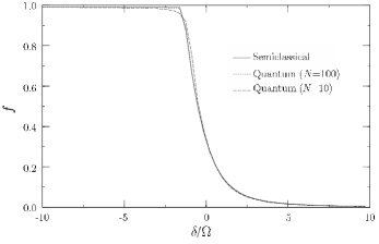
Figure 1: Fraction of atoms forming molecules, $f$, in the ground state of the atom-molecule condensate as a function of the detuning of the laser from photoassociation threshold, $\delta$. The long-dashed and short-dashed lines are from the two-mode quantum treatment for the respective atom numbers $N=10$ and $N=100$, the solid line is from the semiclassical approach embodied in the Gross-Pitaevskii equations.

The idea is near that, when the laser is swept from a large above-threshold detuning to a large (in absolute value) below-threshold value, the system will follow adiabatically, and an atomic condensate is converted to a molecular condensates JAV99 . Moreover, if $\Omega$ were the relevant frequency scale, adiabaticity means that the detuning must change by $\Omega$ in a time of the order or longer than $\Omega^{-1}$. In our model we assume that the detuning is swept as

$$\delta(t)=-\xi\Omega^{2}t\,.$$ (30)

We expect adiabatic following when $\xi\stackrel{{\scriptstyle<}}{{\scriptstyle\sim}}1$.

This piece of intuition is correct. In Fig. 2 we reproduce the relevant figure from Ref. JAV99 . We fix $N=100$. At an initial time giving $\delta=-20\,\Omega$, we start the system in its ground state, almost purely atoms, and integrate the time dependent Schrödinger equation numerically while sweeping the detuning at two rates $\xi=1$ and $\xi=0.1$. The plot gives the fraction of atoms converted to molecules as a function of the instantaneous detuning. For $\xi=1$ we expect to be somewhere at the borderline of adiabaticity, and actually find a conversion efficiency of 0.8. When the laser tuning is swept ten times more slowly, $\xi=0.1$, the conversion efficiency has reached 0.97.

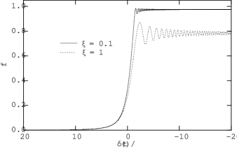
Figure 2: Fraction of atoms converted to molecules, $f=2\langle b^{\dagger}b\rangle$, as a function of instantaneous detuning, $\delta(t)$, when the detuning is swept linearly as a function of time according to $\delta(t)=-\xi\Omega^{2}t$. The figure is for the atom number $N=100$, for the two sweep rates $\xi=0.1$ and $\xi=1$.

We believe that we have discovered a feasible method for preparing a molecular condensate: start with an atomic condensate and a photoassociating laser, then sweep the frequency of the laser in a proper way, and obtain a molecular BEC. In the general manner of adiabatic methods, this “rapid adiabatic passage” should be robust.

Besides its potential utility, rapid adiabatic passage is another example of coherent phenomena that occur in a condensate but not in a nondegenerate gas. Once more, in a nondegenerate gas the frequency scale for adiabaticity is $\kappa$, and the time scale is proportional to $\kappa^{-1}\propto V^{1/2}$. Even if nothing else went wrong, in the limit of a large sample the time scale for adiabatic atom-molecule conversion would tend to infinity. Once more, Bose enhancement saves the day by turning the volume dependence of the relevant frequency scale into a density dependence MAC00a .

IV Field theory for all modes

If only one spatial mode has to be considered for both the atomic and the molecular condensate, the two-mode Hamiltonian (15) is all there is to it. Nonetheless, even if somehow the infinite homogeneous condensate could be approximated in practice, for whatever reason there would always be atoms and molecules present with momenta that are not included in the two-mode picture. As the full Hamiltonian (12) mixes momenta nonlinearly, the possibility of instability arises and should be investigated.

We will study deviations from the two-mode picture, or the possibility that the (infinite) atomic and molecular condensates are not spatially homogeneous. Here we use the quantum field version of our photoassociation theory. But solving nonlinear quantum field theories is generally not a simple matter, and one must approximate. We will resort to classical field theory, the same way one proceeds when an alkali condensate is analyzed using the Gross-Pitaevskii equation.

IV.1 Gross-Pitaevskii equations

To derive the Gross-Pitaevskii equations (GPE) for this problem, in the usual way we first amend the Hamiltonian by adding to it a multiple of the conserved particle number

$$N=\sum_{\bf k}(a^{\dagger}_{\bf k}a_{\bf k}+2b^{\dagger}_{\bf k}b_{\bf k})=\int d^{3}r\,[\phi^{\dagger}({\bf r})\phi({\bf r})+2\psi^{\dagger}({\bf r})\psi({\bf r})]\,.$$ (31)

Instead of the Hamiltonian density, we then use the “Kamiltonian” density

$${\cal K}({\bf r})={\cal H}({\bf r})-\mu[\phi^{\dagger}({\bf r})\phi({\bf r})+2\psi^{\dagger}({\bf r})\psi({\bf r})]\,$$ (32)

in our calculations. This substitution has no effect on the dynamics. At this point the real scalar $\mu$ is arbitrary. Though this piece of knowledge has no bearing on our analysis, in the end the constant $\mu$ will be analogous to chemical potential in thermodynamics. Hence, $\mu$ is called the chemical potential.

Using the standard commutators for boson fields, the Heisenberg equation of motion for the molecular field becomes

$$i\dot{\psi}({\bf r}) = [\psi({\bf r}),\int d^{3}r^{\prime}\,{{\cal K({\bf r}^{\prime})}\over\hbar}\,]$$

$$= \left[-{\hbar\nabla^{2}\over 4m}+\delta_{0}-2{\mu\over\hbar}\right]\psi({\bf r})-\hbox{$1\over 2$}{\cal D}({\bf r})\phi({\bf r})\phi({\bf r})\,.$$

The transformation to the classical field theory is effected by positing that the fields in the equations of motion are no longer boson fields, but commuting $c$-number fields. The interpretation is that $\phi({\bf r})$ and $\psi({\bf r})$ are the macroscopic wave functions for atomic and molecular condensates.

From this point onward we again take the driving field to be a simple plane wave with the positive frequency part $\hbox{$1\over 2$}{\bf E}e^{i{\bf q}\cdot{\bf r}}$. Second, we scale the atomic and molecular fields with the square root of density, $\sqrt{N/V}$. Third, we incorporate the spatial variation of the electric field into the definition of the molecular field. Altogether, we define new atomic and molecular fields $\Phi$ and $\Psi$ as

$$\phi=\sqrt{N\over V}\,\Phi,\qquad\psi=\sqrt{N\over V}\,e^{i{\bf q}\cdot{\bf r}}\Psi\,.$$ (34)

The net results are four. First, the normalization of the fields now reads

$${1\over V}\int d^{3}r\,(|\Phi|^{2}+2|\Psi|^{2})=1\,.$$ (35)

Second, the coefficient $\cal D$ gets multiplied by the square root of the atom density that would prevail if all molecules were to dissociate. Third, all explicit position dependence disappears from the equations of motion. The GPE for the rescaled atomic and molecular wave functions are

$$i\dot{\Phi}({\bf r}) = \left[-{\hbar\nabla^{2}\over 2m}-\mu\right]\Phi({\bf r})-e^{-i\varphi}\Omega\,\Phi^{*}({\bf r})\Psi({\bf r}),$$ (36)

$$i\dot{\Psi}({\bf r}) = \left[-{\hbar\over 4m}\nabla^{2}+i{\hbar\over 2m}{\bf q}\cdot\nabla+\delta-2{\mu\over\hbar}\right]\Psi({\bf r})$$ (37)

$$-\hbox{$1\over 2$}e^{i\varphi}\Omega\,[\Phi({\bf r})]^{2}\,.$$

None other than our characteristic frequency scale for photoassociation, $\Omega$ of Eq. (27), is now explicitly the frequency scale in the field equations as well. The phase factor $e^{i\varphi}$ accounts for the phases of the electric field and dipole moment, and will soon prove inconsequential. Fourth, a photon recoil term got added to the kinetic energy of the molecules.

While still using full dimensional units, we pause to discuss the mathematical symmetries of the GPE. First, a trivial phase change of one of the fields, e.g., $\Phi\rightarrow e^{-i\varphi/2}\Phi$, converts Eqs. (IV.1) to the same equations, except that the phase factors vanish from atom-molecule interaction terms. Therefore, we drop the phase in the interaction term. Second, the GPE have a global gauge invariance. If the fields $\Phi$, $\Psi$ are a solution, then so are the fields $\Phi e^{i\varphi}$, $\Psi e^{2i\varphi}$ for an arbitrary fixed phase $\varphi$. In particular, putting $\varphi=2\pi$, one may see that the equations are invariant under the change of the sign of the field $\Phi$. Third, as a time dependent generalization of the gauge invariance, the GPE is invariant under the replacement

$$\Phi \rightarrow \Phi e^{i\Delta\mu t},$$ (38)

$$\Psi \rightarrow \Psi e^{2i\Delta\mu t},$$ (39)

$$\mu \rightarrow \mu+\Delta\mu\,.$$ (40)

Fourth, the GPE is Galilei invariant, in that the replacements

$$\Phi({\bf r},t) \rightarrow e^{i{\bf k}\cdot{\bf r}}\Phi\left({\bf r}-{\hbar{\bf k}\over m}t,t\right),$$ (41)

$$\Psi({\bf r},t) \rightarrow e^{2i{\bf k}\cdot{\bf r}}\Psi\left({\bf r}-{\hbar{\bf k}\over m}t,t\right),$$ (42)

$$\mu \rightarrow \mu+{\hbar^{2}{\bf k}^{2}\over 2m}\,,$$ (43)

$$\delta \rightarrow \delta-{\displaystyle\hbar{\bf k}\over\displaystyle m}\cdot{\bf q}$$ (44)

convert a solution into another solution that corresponds to an added momentum $\hbar{\bf k}$ per atom. The nontrivial part of the transformation, Eq. (44) is that, due to the Doppler shift, the effective detuning changes depending on the overall motion of the atom-molecule system.

Finally, we express the GPE (IV.1) in a specific system of units,

$$t_{0}={1\over\Omega},\quad r_{0}=\sqrt{\hbar\over m\Omega},\quad m_{0}=m\,,$$ (45)

for time, length and mass respectively. Technically, we should rename the scaled variables and parameter; say, $t=\bar{t}\,t_{0}$, $\delta=\bar{\delta}/t_{0}$. However, we eschew such a heavy notation, and continue to use, e.g., the symbol $\delta$ for what now stands for a dimensionless number and should be properly denoted by $\bar{\delta}=\delta/\Omega$. The result is

$$i\dot{\Phi} = \left[-\hbox{$1\over 2$}\nabla^{2}-\mu\right]\Phi-\Phi^{*}\Psi,$$ (46)

$$i\dot{\Psi} = \left[-\hbox{$1\over 4$}\nabla^{2}+\hbox{$1\over 2$}i{\bf q}\cdot\nabla+\delta-2\mu\right]\Psi-\hbox{$1\over 2$}\Phi^{2}\,.$$ (47)

The GPE equations are as stated in Ref. JAV99a . The plan now is to analyze them. Of course, equations of the type (IV.1) are standard fare in studies of second-harmonic generation. The literature once more is extensive, and we will only give a few specific pointers as we go along.

IV.2 Steady state of GPE

Atomic and molecular fields $\Phi$ and $\Psi$ represent a stationary state, one in which the physics does not change with time, if and only if their time evolution is solely in global (position independent) phase factors, possibly different ones for $\Phi$ and $\Psi$. Now consider fields of the form $\Phi({\bf r},t)=\Phi({\bf r})e^{-i\omega t}$ and $\Psi({\bf r},t)=\Psi({\bf r})e^{-2i\omega t}$ for any real $\omega$. One sees right away that for this type of evolution, at least the exponential time dependence properly matches on both sides of Eqs. (IV.1). Although we have not been able to prove it mathematically, we conjecture that, assuming time independent parameters in Eqs. (IV.1), this type of time dependence is also the only possible case in which the physics is independent of time.

But then, by virtue of the transformation (IV.1), by readjusting the chemical potential one can always remove the time dependence of the fields entirely in any stationary state. The chemical potential started its life as an arbitrary parameter. From now on we make use of the arbitrariness and choose the value in such a way that in steady state the atomic and molecular fields are literally constants in time.

We shall see shortly that, for any time independent detuning $\delta$, one may pick a suitable value for the chemical potential $\mu$ so that the GPE (IV.1) have solutions $\Phi_{0}$, $\Psi_{0}$ that are constants in both space and time. But by virtue of the Galilean transformation (IV.1), we may then construct from $\Phi_{0}$, $\Psi_{0}$ a stationary solution corresponding to an arbitrary overall flow of atoms and molecules, solutions of the form $\Phi\propto e^{i{\bf k}\cdot{\bf r}}$ and $\Psi\propto e^{2i{\bf k}\cdot{\bf r}}$. Conversely, we believe that all spatially homogeneous stationary solutions are such Galilean boosts of the once-and-for-all constant solutions $\Phi_{0}$, $\Psi_{0}$. As far as it comes to spatially homogeneous steady states, we therefore may, and will, without any restriction on generality consider fields that are constants in space and time.

In the context of second-harmonic generation it is well known that the GPE may have spatially inhomogeneous solitary-wave type stationary solutions HE96 . By applying the Galilean transformation, one may find traveling solitary waves as well. Here we will make no effort to find, let alone classify, solitary-wave solutions to our GPE, but proceed as if the homogeneous steady states were all there is to it.

Within the scope of the present paper, the stationary solutions thus satisfy

$$0 = -\mu\Phi_{0}-\Phi^{*}_{0}\Psi_{0},$$ (48)

$$0 = (\delta-2\mu)\Psi_{0}-\hbox{$1\over 2$}\Phi_{0}^{2}$$ (49)

$$1 = |\Phi_{0}|^{2}+2|\Psi_{0}|^{2}\,,$$ (50)

where the final equation originates from the normalization (35). Moreover, by virtue of the global gauge invariance, one may choose $\Phi_{0}$ real. Next, because of the invariance of the GPE with respect to the sign change of $\Phi$, we may always choose $\Phi_{0}$ to be nonnegative. Furthermore, if $\Phi_{0}>0$, then (48) shows that $\Psi$ (like $\mu$) must be real. On the other hand, if $\Phi_{0}=0$, $\Psi_{0}$ comes with an arbitrary phase, and may be chosen real. All told, we only need to find the real solutions $\Phi_{0}$, $\Psi_{0}$, $\mu$ to Eqs. (IV.2), and besides only solutions with $\Phi_{0}\geq 0$ need be retained.

There are three distinct solutions. The trivial one reads

$$\Phi_{0}^{0}=0,\quad\Psi_{0}^{0}=\hbox{$1\over\sqrt{2}$},\quad\mu^{0}=\hbox{$1\over 2$}\delta\,;$$ (51)

for $\delta\leq\sqrt{2}$ we have

$$\Phi_{0}^{+} = {\sqrt{6-\delta^{2}-\delta\sqrt{6+\delta^{2}}}\over 3},$$

$$\Psi_{0}^{+} = {-\delta-\sqrt{6+\delta^{2}}\over 6},$$

$$\mu^{+} = -\Psi_{0}^{+}\,;$$ (52)

and for $\delta\geq-\sqrt{2}$ we find

$$\Phi_{0}^{-} = {\sqrt{6-\delta^{2}+\delta\sqrt{6+\delta^{2}}}\over 3},$$

$$\Psi_{0}^{-} = {-\delta+\sqrt{6+\delta^{2}}\over 6},$$

$$\mu^{-} = -\Psi_{0}^{-}\,.$$ (53)

At least two steady states are found for each $\delta$, and three in the interval $-\sqrt{2}<\delta<\sqrt{2}$. The question is, which one represents the desired physical steady state. Here we attempt to mimic the ground state of the quantum-mechanical two-mode model (15), and choose the stationary solution so that JAV99a

$$\delta<-\sqrt{2} : \Phi_{0}=\Phi_{0}^{0},\Psi_{0}=\psi_{0}^{0},\mu=\mu^{0},$$

$$\delta\geq-\sqrt{2} : \Phi_{0}=\Phi_{0}^{-},\Psi_{0}=\psi_{0}^{-},\mu=\mu^{-}\,.$$ (54)

The success is evident in Fig. 1, where we plot side by side the fraction of atoms converted to molecules from the quantum-mechanical two-mode model and the corresponding GPE approximation $f=2\Psi_{0}^{2}$ (solid line) as a function of detuning. By comparing with the $N=10$ and $N=100$ quantum results, it may be seen that the agreement between the GPE and the quantum approach gets better as the number of atoms is increased. Even for an atom number as small as 100 and around the nonanalytic point $\delta=-\sqrt{2}$ of the GPE approximation (54), the difference is only on the order of one per cent.

We conclude by noting that Eqs. (51) and (52) together give a stationary solution that is the exact mirror image of our choice (54) with the substitution $\delta\rightarrow-\delta$. This corresponds to the state with maximum energy for the two-mode quantum system. It is a stationary state just as is the minimum, and may be used for atom-molecule conversion. The difference is that, in the case of the maximum, the detuning would be swept in the opposite direction, from below to above the dissociation threshold. Otherwise rapid adiabatic passage should work essentially as before.

IV.3 Small excitations of the system

So far, while analyzing the GPE, we have achieved nothing more than in our studies of the two-mode model; rather less, because in our classical field theory we lose quantum fluctuations. Nevertheless, we now have the tools to analyze the stability of the steady state, and see how spatial inhomogeneities evolve in time.

As in Ref. JAV99a , we linearize the GPE around a stationary solution, and then attempt to find eigenmodes for small deviations from the stationary case. Both of these steps are achieved at once by inserting the Ansatz

$$\Phi({\bf r},t)=\Phi_{0}+u_{\Phi}\,e^{i({\bf p}\cdot{\bf r}-\omega t)}+v^{*}_{\Phi}\,e^{-i({\bf p}\cdot{\bf r}-\omega^{*}t)}$$ (55)

into the GPE, and only retaining the first-order terms in the “small” coefficients $u_{\Phi}$, $v_{\Phi}$. Of course, the field $\Psi$ is treated similarly. We need to mix plane waves ${\bf p}$ and $-{\bf p}$ because the GPE mixes fields and their complex conjugates. With our Ansatz we also retain the possibility that the evolution frequency of an eigenmode could be complex.

The Ansatz succeeds if the as of yet unknown evolution frequency $\omega$ satisfies the eigenvalue equations

$${\left[-\hbox{$1\over 2$}{{\bf p}}^{2}+\mu+\omega\right]{u}_{\Phi}+\psi_{0}{v}_{\Phi}+\Phi_{0}{u}_{\Psi}=0,\quad}$$ (56)

$${\left[-\hbox{$1\over 2$}{{\bf p}}^{2}+\mu-\omega\right]{v}_{\Phi}+\psi_{0}{u}_{\Phi}+\Phi_{0}{v}_{\Psi}=0,\quad}$$ (57)

$${\left[-\hbox{$1\over 4$}({\bf p}^{2}+2{\bf p}\cdot{\bf q})+2\mu-{\bar{\delta}}+\omega\right]{u}_{\Psi}+\Phi_{0}{u}_{\Phi}=0,\quad}$$ (58)

$${\left[-\hbox{$1\over 4$}({\bf p}^{2}-2{\bf p}\cdot{\bf q})+2\mu-{\bar{\delta}}-\omega\right]{v}_{\Psi}+\Phi_{0}{v}_{\Phi}=0.\quad}$$ (59)

The characteristic equation is fourth order in $\omega$, so in principle the solutions can always be written down analytically. However, here we use Mathematica MATHEMATICA to produce results directly numerically, and occasionally to extract analytical forms for special and limiting cases.

The dispersion relations of the excitation modes, $\omega=\omega({\bf p})$, depend on the relative propagation directions of the excitation and of light, and also on the size of the photon recoil kick. We encompass these dependences into a dimensionless parameter, which in terms of the original dimensional parameters reads

$$\eta=\sqrt{\hbar({\bf q}\cdot{\bf p})^{2}\over m\Omega\,{\bf p}\cdot{\bf p}}\,.$$ (60)

Given the parameter $\eta$ and the absolute value $p$ of the (dimensionless) propagation vector ${\bf p}$, the terms that depend on photon recoil in Eqs. (IV.3) are replaced as follows,

$$\hbox{$1\over 4$}({\bf p}^{2}\pm 2{\bf p}\cdot{\bf q})\rightarrow\hbox{$1\over 4$}(p^{2}\pm 2\eta p)\,.$$ (61)

For fixed values of the parameters $\delta$, $\eta$ and $p$, there are four excitation modes with four (in general) different evolution frequencies $\omega$. If a positive imaginary part is encountered in any one of the four frequencies, the corresponding mode grows exponentially and the steady state is unstable.

Let us take the wave vector characterizing the small-excitation mode to be perpendicular to the propagation direction of light, $\eta=0$. We begin with $p=0$ and assume $|\Psi_{0}|^{2}<\hbox{$1\over 2$}$, a nontrivial mix of atoms and molecules. We find the solutions to the characteristic equation for the eigenvalue problem (IV.3)

$$\omega_{1}^{2}(0) = 0.$$ (62)

$$\omega_{2}^{2}(0) = \left(3+{1\over 2|\Psi_{0}|^{2}}\right)\left({1\over 2}-|\Psi_{0}|^{2}\right)\,.$$ (63)

When the wave number of the excitation moves away from $p=0$, of the four frequencies the two evolving continuously from $\pm\omega_{2}(0)$ remain real. Their dispersion relations for small $p$ are of the type $\omega_{2}(p)\simeq\omega_{2}(0)+{1\over 2m^{*}}p^{2}$, with $m^{*}\geq 0$, so that these excitations are akin to optical phonons. On the other hand, the remaining two excitation frequencies are either purely real or purely imaginary, and for small enough $p$ they are always imaginary. Such modes do not propagate at all, but grow or shrink in place exponentially.

In fact, in Fig. 3, which is transcribed from Ref. JAV99a , we plot the largest imaginary part among the four frequencies $\omega$, $|\Im[\omega_{1}]|$, as a function of the detuning $\delta$ and the wave number $p$ of the excitation mode. As above, we set $\eta=0$. It may be seen that, for any detuning $\delta>-\sqrt{2}$, an unstable excitation mode is always found. The largest imaginary part of an evolution frequency, i.e, the largest growth rate of an instability, is encountered at $\delta=-0.154496$ and $p=\pm 0.771324$, and equals $\Im(\omega)=0.24256$.

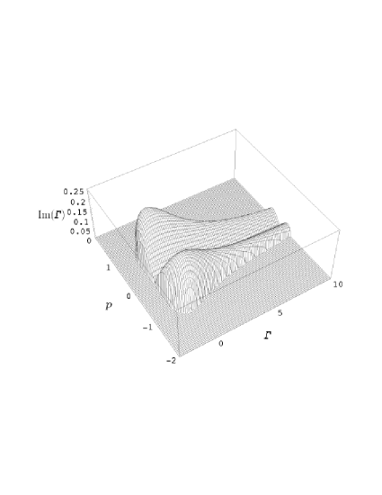
Figure 3: Largest imaginary part among the four evolution frequencies of small perturbations of the joint atom-molecule condensate is plotted as a function of the laser detuning $\delta$ and the wave number of the plane-wave like perturbation $p$. In this figure the excitation mode propagates perpendicularly to the propagation direction of light, so that $\xi=0$.

The analogous instability is naturally known in second-harmonic generation, and goes under the rubric “modulational instability” TRI95 ; HE96a .

We next come to the effect of the direction of the wave vector of the mode on instability. In Fig. 4 we plot the largest positive imaginary part of a mode frequency found for any $p$ as a function of the parameter $\eta$. The curves are labeled with their corresponding fixed detunings $\delta$. In our studies of this kind, the largest growth rate of the instability was always found for $\eta=0$. For a given detuning, the small excitations whose momentum direction is perpendicular to light propagation always present the most unstable scenario.

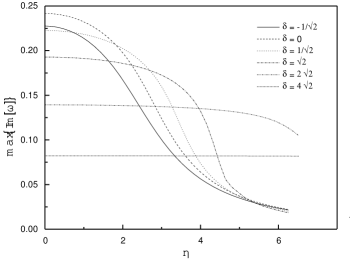
Figure 4: Largest imaginary part in a small-excitation evolution frequency encountered for any value of the wave number of the excitation $p$ is plotted against the parameter $\xi$ that characterizes the component of the photon recoil momentum in the direction of the propagation vector of the small excitation ${\bf p}$. The explicit definition of $\xi$ is given in Eq. (60). Different curves are for different fixed detunings $\delta$, as identified in the legend.

Finally consider the largest growth rate of the instability (among all ${\bf p}$) as a function of the detuning. As may be inferred from Fig. 3, with increasing detuning $\delta\stackrel{{\scriptstyle>}}{{\scriptstyle\sim}}1$ it decreases and occurs at smaller momenta, i.e., at larger size scales. In fact, for $\delta\gg 1$, the maximum growth rate of an instability $R(\delta)=\max\{\Im[\omega(p,\delta)]\}_{p}$ behaves as

$$R(\delta)\sim\left[{1\over 2\,\delta}-{5\over 4\,\delta^{3}}+{\cal O}({1\over\delta^{5}})\right],$$ (64)

and the corresponding position of the maximum $p_{M}(\delta)$, the value of the momentum such that $\Im[\omega(p,\delta)]\leq\Im[\omega(p_{M},\delta)]$ for all $p$, goes like

$$p_{M}(\delta)\sim\sqrt{1\over\delta}\,\left[1-{1\over\delta^{2}}+{47\over 16\,\delta^{4}}+{\cal O}({1\over\delta^{6}})\right]\,.$$ (65)

Of course, as the largest growth rate of the instability seems to occur for $\eta=0$, this was our choice in Eqs. (64) and (65).

In sum, we have found that for $\delta\leq-\sqrt{2}$ the steady state of the atom-molecule system is stable, and for any $\delta>-\sqrt{2}$ it is unstable. Although we have reported only on a specific stationary solution (54), possibly one out of three, the modes we have not considered explicitly are all unstable. But $\delta=-\sqrt{2}$ is also the watershed, in that below $\delta=-\sqrt{2}$ the steady state is all molecules ($\Phi_{0}=0$), and above $\delta=-\sqrt{2}$ some atoms are involved. All told, the steady state with everything in molecules is stable for $\delta\leq-\sqrt{2}$, but any steady state involving atoms is always unstable. The most unstable situation occurs around $\delta\simeq 0$, with about an equal mixture of atoms and molecules. For $\delta\gg 1$ atoms take over, and the time scale for the instability grows longer.

IV.4 Fate of unstable system

Linearized stability analysis has shown that a joint atom-molecule condensate is unstable in the presence of photoassociating light, i.e., there are small-excitation modes that grow exponentially. But when a small deviation from steady state grows exponentially, eventually it is not a small deviation anymore and the linearized analysis breaks down. To investigate the fate of the system once the instability has set in, we integrate the full GPE numerically as in Ref. JAV99a . Our aim is a qualitative demonstration, so we proceed in $1+1$ dimensions, one spatial coordinate $x$ and time $t$. However, there is nothing in our method that would not immediately work in higher spatial dimensions. The restriction is merely a matter of computer time.

Specifically, in our algorithm we discretize a stretch $L$ of the line into equidistant points $x_{i}$, and seek to represent the fields at these discrete points only. For convenience, we use periodic boundary conditions, so that the value of all functions repeats over $L$. The GPE is integrated over a time step $h$ in two moves. First we ignore the position derivatives in the GPE altogether. This implies that the stripped-down version of the GPE is local; for each $x_{i}$, $\Phi(x_{i})$ and $\Psi(x_{i})$ only couple to $\Phi(x_{i})$ and $\Psi(x_{i})$. We integrate the local version of the GPE over the time $h$ separately for each $x_{i}$ as two coupled differential equations using a second-order Runge-Kutta step. To prevent a numerical drift of the norm, we complete the initial step of the algorithm by normalizing the fields analogously to Eq. (35). Second, we ignore anything but the position derivatives in the GPE. The resulting partial version of the GPE is nonlocal, but in exchange it is linear and does not mix the fields $\Phi$ and $\Psi$. To integrate over the same (sic!) time step as in the initial part of the algorithm, we first take the Fourier transform of the result from the first part using the Fast Fourier Transformation (FFT). In Fourier space position derivatives become local, so, to propagate the fields over the step $h$, we simply multiply their Fourier transforms by what is now the local, exact (within FFT), linear time evolution operator. Finally, in preparation for the next step, we transform back to real space.

This split-step algorithm is an obvious variation of the time honored split-operator methods for linear partial differential equations SPLITSTEP , and has been described before at least by the group of Firth SKR98 . Nonetheless, it comes with a fair dose of heuristics. It is therefore gratifying that we have been able to verify a good rate of convergence by using successively smaller time steps to integrate over a fixed interval of time.

We present an example of our simulations in Fig. 5, showing the absolute square of the atomic field $|\Phi|^{2}$ as a function of position $x$ and time $t$. We use 128 points $x_{i}$. Because of the periodic boundary conditions, the left and right edges of $x$ wrap around and are actually the same. The plot is for the parameters $\delta=0$, $\eta=0$, the range of position $x$ is 24.6282 (in units of $r_{0}$) corresponding to three wavelengths of the most unstable excitation mode for these parameters, and time $t$ runs from 0 to 127 (in units of $t_{0}$). The unit of $|\Phi|^{2}$, atom density, is such that for a homogeneous gas with everything in atoms, the density would be $|\Phi|^{2}\equiv 1$. The system starts at time $t=0$ in the steady state appropriate for $\delta=0$, $\eta=0$, except that we add a small amount of Gaussian noise to each of the points specifying the initial state. Figure 5 is otherwise the same as Fig. 2 in Ref. JAV99a , except that a different seed was used for the random number generator that added the noise. As befits an instability, this innocuous change has lead to a totally different quantitative result at long times.

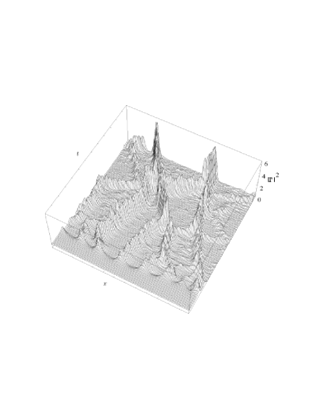
Figure 5: An example to demonstrate the modulational instability of the joint atom-molecule condensate. Atom density $|\Phi|^{2}$ is plotted as a function of the spatial coordinate $x$ and time $t$, given that the system starts out at time $t=0$ in the steady state plus a small amount of random noise.

From the numerical simulations we see that the nature of the instability is such that the atoms and the molecules together combine into dense clumps. These clumps move around, and tend to join when they collide. As far as we can tell, within the present model only one big, dense clump will remain in the end.

One might wonder what is the mechanism behind the clumping. We present a heuristic guess. We are not talking about a thermodynamic system, so minimization of energy is a dubious principle to begin with; and besides, we are dealing with quasienergies in a rotating frame, not real energies. With these warnings out of the way, let us surmise that the system nevertheless attempts to minimize its energy. The atomic and molecular condensates make something akin to the two-level system in quantum optics. When light is added, one gets a dressed two-level system. The energy of the lower one of the two dressed states decreases with increasing Rabi frequency, which is the product of the electric field strength of the laser and the dipole moment. But the analog of Rabi frequency for the two-level system of atomic and molecular condensates, $\Omega$, is also proportional to the square root of density, so the present system may also decrease its energy by increasing the density. Maybe this is what the instability is about.

V Experimental considerations

The models we have discussed until now have been rather rudimentary. We next take up two types of complications that may come up in experiments. First, in Sec. V.1 enters an angle that is in principle included in our many-body Hamiltonian, although we have not yet considered it expressly: photodissociation of condensate molecules to states outside of the atomic condensate. It turns out to limit the rate at which one can achieve coherent atom-molecule conversion in adiabatic passage. Second, in Sec. V.2 we discuss a number of aspects that have so far been missing from our models: spontaneous emission from the photoassociated state, atom-atom interactions, trapping of atoms and molecules, and various level shifts. Spontaneous emission can be ameliorated by resorting to a two-color photoassociation scheme. Provided that photoassociation is speedy enough, which we believe is technically possible, the rest of these complications may be minor nuisances rather than dominant features of an experiment. What it takes to make photoassociation speedy enough is the subject of Sec. V.3, where we discuss the characteristic Rabi frequency for photoassociation $\Omega$ for various alkalis. Finally, in Sec. V.4, we analyze the published experiment of Ref. WYN00 from our viewpoint of coherent photoassociation.

V.1 Rogue photodissociation

As we noted already, in the case of photoassociation of an infinite homogeneous condensate, momentum conservation uniquely determines the state of the ensuing molecule. The converse, however, does not hold. When a molecule photodissociates into two atoms, momentum conservation does not force the atoms to return to the atomic condensate. Bose enhancement favors recombination of atoms with the condensate; the characteristic frequency is $\Omega$ for both photoassociation and photodissociation between atomic and molecular condensates. Nonetheless, atoms winding up elsewhere are lost for coherent photoassociation. We have coined the term “rogue photodissociation” for photodissociation processes that send atoms outside the atomic condensate.

One might think that energy conservation in the cycle of photoassociation and photodissociation is the additional constraint that guarantees that the atoms return to the condensate. But this need not be a compelling argument. Any time dependence in the system interferes with energy conservation. For instance, suppose that photodissociation proceeds to the noncondensate states at the same rate $\Gamma_{0}$ (per atom) as it would in the case of a nondegenerate gas of molecules, so that after a time $\sim\Gamma_{0}^{-1}$ coherent photoassociation ceases. The photodissociation rate $\Gamma_{0}$ in itself furnishes a time scale such that energy has to be conserved only to within $\hbar\Gamma_{0}$. The time evolution involved in nonlinear Rabi flopping would also interfere with energy conservation.

We present here a rudimentary model for rogue photodissociation for the special case when the detuning is swept in order to convert an atomic condensate to a molecular condensate. The key assumption is that we may employ the standard Markov approximation in the analysis of photodissociation. This entails that rogue photodissociation has no memory, but is characterized at each instant of time by a rate of exponential decay. Such an assumption seems dubious in particular when the laser is tuned to the close vicinity of the photodissociation threshold RZA82 . However, we know of no near-threshold case of this kind in which the breakdown of the Markov approximation has proven relevant in an experiment.

Evidently, only the condensate mode, one of very many atomic modes, is strongly affected by Bose enhancement. We take rogue photodissociation to proceed at the rate that would be appropriate for a nondegenerate gas at the given detuning. Second, we model the dependence of the photodissociation rate on detuning using the Wigner threshold law, so that we write

$$\Gamma(\delta)=\theta(\delta)\,\sqrt{\delta\over\Omega}\,\Gamma_{0}\,.$$ (66)

For convenience we have chosen the photoassociation frequency scale $\Omega$ as the reference detuning for photodissociation rate; $\Gamma_{0}$ is the photodissociation rate for the detuning $\delta=\Omega$. As the third quantitative element of the model, we take the probability that a given atom is in the molecular condensate to be twice the square of the molecular field amplitude as solved from the classical field theory, and normalized as in (50). Explicitly, in dimensional units and for $\delta\geq 0$, this probability is found from Eq. (53) as

$$P_{M}(\delta)={1\over 18}\left[-\left({\delta\over\Omega}\right)+\sqrt{6+\left({\delta\over\Omega}\right)^{2}}\right]^{2}$$ (67)

Suppose now that the detuning is swept as $\delta=-\xi\Omega^{2}t$, as in our rapid adiabatic passage example. Ignoring the depletion of the condensates due to the very same rogue photodissociation, we find the total probability for rogue photodissociation

$$P = \int_{\delta(t)\geq 0}dt\,P_{M}[\delta(t)]{\,\Gamma_{0}\sqrt{\delta(t)\over\Omega}}$$ (68)

$$= {\Gamma_{0}\over\xi\Omega}\left[{2^{3/4}\over 3^{1/4}}\int_{0}^{\infty}d\tau\,\sqrt{\tau}\left(\sqrt{1+\tau^{2}}-\tau\right)^{2}\right]$$

$$= \alpha\,{\Gamma_{0}\over\xi\Omega}\,,$$

where the numerical constant has the value $\alpha=4.03197$. Except for the numerical factor, this is the same expression we already used in a qualitative estimate in Ref. JAV99 .

Since the photodissociation rate grows linearly with light intensity, $\propto I$, and the photoassociation characteristic frequency $\Omega$ is proportional to the field strength of the laser, $\propto\sqrt{I}$, in the end rogue photodissociation wins out as the light intensity is increased. Qualitatively, when $P=1$, rogue photodissociation has overtaken coherent conversion of atoms to molecules. To study this borderline case, we first set $P=1$ in Eq. (68) and solve $\Gamma_{0}$ as a function of $\Omega$. We then insert the result into Eq. (27), thus eliminating $\Gamma_{0}$. Moreover, the velocity $v_{0}$ in Eq. (27) is then the relative velocity of the dissociated atoms corresponding to the detuning of the laser that gave the photoassociation rate $\Gamma_{0}$, in this case $\delta=\Omega$. Therefore we have $v_{0}^{2}/2\mu=\hbar\Omega$, and $v_{0}$ may be eliminated as well. We finally solve for the borderline value $\Omega$ as a function of the problem parameters. After simple manipulations the ensuing characteristic frequency scale for photoassociation may be written

$$\hat{\Omega}=\left({8\sqrt{2}\pi\xi\over\alpha}\right)^{2/3}\,(\rho\lambdabar^{3})^{2/3}\,\epsilon_{R}\,.$$ (69)

Here we have introduced $\lambdabar$, wavelength of the light divided by $2\pi$, and the familiar recoil frequency for laser cooling

$$\epsilon_{R}={\hbar\over 2m\lambdabar^{2}}\,.$$ (70)

The main finding is that rogue photodissociation restricts the light intensity that one may profitably use for adiabatic atom-molecule conversion. This means that there is also a maximum usable photoassociation frequency, or a minimum possible time scale for adiabatic atom-molecule conversion. The way we have written our estimate (69), the frequency scale is provided by the photon recoil frequency, and the corresponding time scale is in the ballpark of $\epsilon_{R}^{-1}$. The density dependence of photoassociation is encapsulated in the parameter $\rho\lambdabar^{3}$, the usual dimensionless parameter that governs the coupling of light with matter in a dense medium. For present-day condensates $\rho\lambdabar^{3}\sim~{}1$ is a reasonable rule of thumb. Finally, we have a numerical constant that depends on the rate of sweeping of the detuning, but which may also be set equal to one in a rough estimate. Altogether, when in need of a qualitative number for the photoassociation frequency $\Omega$, we resort to $\Omega\sim\epsilon_{R}$.

Although our estimate of the minimum time scale for coherent photoassociation was developed for rapid adiabatic passage, we believe that (with $\xi\simeq 1$) it also applies to Rabi flopping. This is because the dimensional parameters of the problem are the same in both cases. In fact, as it comes to dimensional quantities, the minimum time scale for coherent photoassociation is equivalently written FOOT

$$\tau\sim{m\over\hbar\rho^{2/3}}\,.$$ (71)

This is the essentially unique quantity with the dimension of time that can be put together using the quantities characterizing a homogeneous, noninteracting, quantum mechanical, zero-temperature BEC; density, atom mass, and $\hbar$.

V.2 Physics missing from model

V.2.1 Spontaneous emission

We have discussed a one-color model for photoassociation. The physical drawback is that, where there is a strong dipole matrix element for photoassociation/dissociation driven by external light, there is also a strong dipole matrix element for spontaneous emission. For instance, if a photon is absorbed in photoassociation, then there is also a reverse spontaneous decay of the molecule. The molecule may end up in bound vibrational states, either in the same electronic manifold where the atoms started from, or in some other electronic manifold. Alternatively, the photoassociated molecule may decay back to a dissociation continuum in a process known as radiative escape. Either way, usually the probability is small that the system returns to the same two-atom state in which is started. After each process of spontaneous emission, two atoms are typically lost for any profitable use.

The analogous problem of an unstable excited state is standard fare in quantum optics, and so is the solution: add another laser-driven transition from the spontaneously decaying state to a stable state. In the same way, two-color Raman photoassociation, a free-bound transition followed by a bound-bound transition of the molecule, may take place between (nearly) non-decaying atomic and molecular states BOH96 ; MAC99 ; BOH99 . Here we study Raman photoassociation as a means of achieving an effective two-mode scheme; genuine three-mode phenomena such as STIRAP are discussed elsewhere MAC00

Our present notation for this scheme is sketched in Fig. 6. Suppose the first step of photoassociation takes place with absorption of a photon, then one sets up another laser to force, say, induced emission from the primary photoassociated state to a (more) stable bound molecular state. We call the Rabi frequency in the second step $\chi$, the detuning of the laser from resonance in the second transition $\Delta$, and the spontaneous decay rate of the primary photoassociation state $\Gamma_{\rm s}$. In this context $\delta$ stands for the two-photon detuning, the total energy mismatch for light-induced transition from the initial atoms to the final stable molecular state, including appropriate photon recoil corrections.

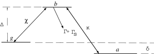
Figure 6: Schematic three-level scheme for photoassociation. The levels $a$, $b$ and $g$ stand for atoms, primary photoassociated molecules, and final stable molecules, respectively. The figure is drawn in the rotating frame, so that the Rabi frequencies $\kappa$ and $\chi$ representing the laser fields are independent of time, and the intermediate and two-photon detunings $\Delta$ and $\delta$ are drawn as appropriate level energies.

Let us model our three-level $\Lambda$ scheme using a variation of the two-mode model (15) as

$${H\over\hbar}=\delta\,g^{\dagger}g+(\Delta\!+\!\delta)b^{\dagger}b-\chi(b^{\dagger}g\!+\!g^{\dagger}b)-\hbox{$1\over 2$}\kappa(b^{\dagger}aa\!+\!ba^{\dagger}a^{\dagger})\,,$$ (72)

where $g$, for “ground”, is the annihilation operator for the stable molecular state. Once more, we have added a multiple of the conserved particle number, this time in such a way that the atoms have zero energy. The term $\propto\chi$ describes transitions between the bound molecular states. Spontaneous losses from the intermediate state are ignored for the time being.

The Heisenberg equations of motion from Hamiltonian (72) are

$$\dot{g} = -i\delta g+i\chi b,$$ (73)

$$\dot{b} = -i(\Delta+\delta)b+i\chi g+\hbox{$1\over 2$}i\kappa aa,$$ (74)

$$\dot{a} = i\kappa a^{\dagger}b\,.$$ (75)

We next eliminate the intermediate state adiabatically with the assumption that $\Delta$ is the largest evolution frequency in the system. We thus formally set $\dot{b}=0$, and obtain

$$b\simeq{\chi g+\hbox{$1\over 2$}\kappa aa\over\Delta}\,.$$ (76)

Inserting this into Eqs. (73) and (75), we have

$$\dot{g} = -i\left(\delta-{\chi^{2}\over\Delta}\right)g+\hbox{$1\over 2$}i\,{\kappa\chi\over\Delta}\,aa,$$ (77)

$$\dot{a} = i\,{\kappa\chi\over\Delta}a^{\dagger}g+\hbox{$1\over 2$}i{\kappa^{2}\over\Delta}a^{\dagger}aa\,.$$ (78)

These are Heisenberg equations of motion for the effective Hamiltonian

$${H_{\rm eff}\over\hbar}=\left(\delta-{\chi^{2}\over\Delta}\right)g^{\dagger}g-\hbox{$1\over 4$}{\kappa^{2}\over\Delta}a^{\dagger}a^{\dagger}aa-\hbox{$1\over 2$}{\kappa\chi\over\Delta}(a^{\dagger}a^{\dagger}g+g^{\dagger}aa)\,.$$ (79)

The effective Hamiltonian describes a two-level system with the two-photon detuning $\delta$ and two-photon Rabi frequency $\kappa\chi/\Delta$ in lieu of the usual detuning and Rabi frequency. There are two additional twists to the story. First, the two-photon resonance experiences a light shift $-\chi^{2}/\Delta$, an old acquaintance from quantum optics. Second, we have an effective atom-atom interaction proportional to $\kappa^{2}/\Delta$. An analogous interaction in a nondegenerate gas was discussed earlier in Ref. SHL96 . Other than these tweaks, everything we have said about the two-mode model applies as before.

The adiabatic elimination (76) has a dark side hidden by a notational trick, namely, that it does not preserve boson commutators. Had we written the right-hand side in Eq. (75) as $ba^{\dagger}$ instead of $a^{\dagger}b$ and substituted (76), the atom-atom interaction term in the effective Hamiltonian would have displayed the operator ordering $aaa^{\dagger}a^{\dagger}$ instead of $a^{\dagger}a^{\dagger}aa$. The difference is immaterial for a large atom number, the limit we are studying anyway, but a more careful investigation of the adiabatic elimination would be in order if the atom number were not large.

As excessive care with operator products is not warranted, we write from the adiabatic assumption the number of atoms in the intermediate state $b$ qualitatively as

$$b^{\dagger}b\sim\left({\chi\over\Delta}\right)^{2}g^{\dagger}g+\left({\kappa\over 2\Delta}\right)^{2}(a^{\dagger}a)^{2}\,.$$ (80)

Let us scale the operators by $\sqrt{N}$, i.e., write $b=\sqrt{N}\beta$, and so forth. Then, within a factor of two, the quantum expectation value $\langle\beta^{\dagger}\beta\rangle$ is the probability that an atom is in the intermediate state, and so on. Equation (80) becomes

$$\beta^{\dagger}\beta\sim\left({\chi\over\Delta}\right)^{2}\gamma^{\dagger}\gamma+\left({\Omega\over 2\Delta}\right)^{2}(\alpha^{\dagger}\alpha)^{2}\,.$$ (81)

The fraction of atoms lost per unit time to spontaneous emission from the intermediate state equals $2\Gamma_{\rm s}\langle\beta^{\dagger}\beta\rangle$.The intermediate detuning $\Delta$ suppresses losses by a factor $\propto 1/\Delta^{2}$, whereas the effective Rabi frequency scales as $1/\Delta$. In principle, and at the present level of the physical model, it is possible to get rid of the harmful spontaneous emission to any desired degree by increasing the intermediate detuning.

V.2.2 Interactions between atoms and molecules

Atoms interact among themselves, molecules interact with molecules, and atoms even interact with molecules. For a dilute gas, the atom-atom interaction is often described by the effective two-body potential

$$U({\bf r}_{1},{\bf r}_{2})={4\pi\hbar^{2}a\over m}\,\delta({\bf r}_{1}-{\bf r}_{2})\,,$$ (82)

where $a$ is the $s$-wave scattering length for the atoms as before. One may write analogous models for atom-molecule and molecule-molecule interactions. If atom-atom interactions were suspected to be a factor, one could add to the field theory the usual two-body atom-atom interactions as

$${\cal H}_{AA}={2\pi\hbar^{2}a\over m}\,\phi^{\dagger}({\bf r})\phi^{\dagger}({\bf r})\phi({\bf r})\phi({\bf r})\,,$$ (83)

and so on. Inelastic collisions, such as quenching of the molecules by collisions, may also prove important. At a phenomenological level, they could be described by using a complex scattering length for atom-molecule collisions.

Nonetheless, we have considered neither elastic nor inelastic collisions explicitly in this paper. The motivation is mainly pragmatic. Photoassociation is the novelty of this work anyway. Second, at this point in time virtually nothing is known about the scattering lengths for cases other than atom-atom interactions. Third, as pointed out in Sec. V.1, we anticipate a characteristic frequency scale for photoassociation, $\Omega$, to be of the order of photon recoil frequency $\epsilon_{R}$ of laser cooling, say, ten kilohertz. This is larger than a typical frequency scale associated with collisions, $4\pi\hbar a\rho/m$, in many of the present alkali experiments. Photoassociation should dominate the action at least over short time scales.

More formally, we see from Eqs. (69) and (71) that the maximum usable photoassociation frequency scales with atom density as $\rho^{2/3}$, while the rate of binary collisions scales as $\rho$. In principle and at this level of modeling, it is always possible to make photoassociation win out by decreasing the density.

Of course, not all of our discussions are for short times only. Notably, in the case of the instability of a joint atom-molecule condensate, it may well happen that collisional interactions eventually play a role in the clumping. We plan to return to collisional effects in a future publication, inasmuch as something worthwhile emerges from this front.

V.2.3 Trapping of atoms

In the current alkali vapor experiments one does not see infinite homogeneous condensates, but the condensate is ordinarily confined to a magnetic trap with a (practically quadratic) potential $V({\bf r})$. This may be taken into account in the field theory by adding a term in the Hamiltonian density,

$${\cal H}_{\rm VA}({\bf r})=\phi^{\dagger}({\bf r})V({\bf r})\phi({\bf r})\,.$$ (84)

A similar additional term would describe trapping of molecules.

In fact, the beauty of the field theoretical formulation is that it does not depend on any given one-particle basis to describe the motion of the atoms and molecules. The photoassociation term was originally discussed using plane-wave states, which makes the derivation easy, but at the level of field theory there is no manifest vestige of plane waves anymore. Even if we add trapping potentials, there is no need to tamper with the photoassociation term. This should be contrasted with the more delicate situation that emerges if one tries to consider photoassociation directly using the eigenstates of the trap, or indeed some states that would take into account both trapping and atom-atom interactions.

Once more, if the photoassociation frequency scale is of the order $\epsilon_{R}$, it is still vastly larger than the typical frequency scales associated with magnetic trapping of atoms, and the corresponding length scale for photoassociation, $\lambdabar$, is far smaller than the size of a typical condensate. Over short times the condensates behave locally as if they were homogeneous. One just applies the theory of an infinite condensates at each local density, and averages the results over the trap.

On the other hand, there are cases in our formulation where the trapping will matter. For $\Omega~{}\sim\epsilon_{R}$ the modulational instability may well set in as in a homogeneous condensate, but the motion of the atoms and molecules due to the trapping forces will certainly have a long-term effect on the atom-molecule clumps. We do not discuss this issue here, but plan to return to trapping in a future publication.

V.2.4 Level shifts

We have already mentioned a few mechanisms that can change the position of the photoassociation resonance. Atom-atom and molecule-molecule interactions alter the energy per atom or per molecule, and thereby modify the resonance condition for photoassociation. Since the atom-molecule ratio conversely depends on the detuning, the makings of bistability and hysteresis are in principle there. We have also discussed the light shift and the many-body shift in a two-color, three-mode configuration.

One more shift we have brought up before JAV98 ; MAC99 , but not yet in this paper, arises because the dissociation continuum is not flat. Given the initial state, the dipole matrix element (or more precisely, the square of the dipole matrix element per unit energy) depends on the final continuum state. The result is that the photodissociation rate picks up an imaginary part. That, of course, amounts to a shift of the photodissociating state with respect to the continuum. The shift is proportional to light intensity, and in a qualitative estimate is comparable to the photodissociation rate; see, e.g., Refs. jav .

Moreover, there are additional shifts due to the presence of each and every discrete state dipole-coupled to the initial state. The sum of all light shifts is actually finite only because the dipole coupling eventually tends to zero when one goes high enough in the energy of the coupled states. The implication is that, a priori, all dipole coupled states, even those off resonance by perhaps several photon energies, have to be considered explicitly. If one finds a significant contribution to the light shift from one far-off resonance state, chances are that one has to consider all of them.

We will not attempt to address continuum and non-resonant light shifts explicitly. Nonetheless, on the basis of the atomic case discussed in Refs. jav , we believe that, at least above the photodissociation threshold, the light shift should be reasonably independent of where exactly the laser is tuned. This would mean that, in the rapid adiabatic passage type atom-molecule conversion, the light shift merely gives a constant bias to the detuning, and is virtually inconsequential.

V.3 Numerical examples

V.3.1 From rate to Rabi frequency

One-color photoassociation has been analyzed by various groups PA-groups , in particular for alkalis at finite temperature. A typical outcome is the photoassociation rate ${\cal R}_{v^{\prime}}$ (in s^-1) or the photoabsorption rate coefficient $\alpha^{PA}_{v^{\prime}}$ (in cm⁵) for a given bound level $v^{\prime}$ of the excited electronic state. The latter quantity is independent of two experimental parameters, namely atom density $\rho$ and laser intensity $I$. The rate of photoassociation ${\cal R}_{v^{\prime}}$ is obtained via

$${\cal R}_{v^{\prime}}=\rho\varphi\alpha^{PA}_{v^{\prime}}\;,$$ (85)

where the photon flux (photons/s cm²) is given by $\varphi=I/\hbar\omega_{L}$, $\omega_{L}$ being the photon frequency.

But we also know from our earlier work JAV98 ; MAC99 that the photoassociation rate in a thermal sample is given in terms of our detuning $\delta$, temperature $T$, and photoassociation rate $\Gamma$ as

$${\cal R}_{v^{\prime}}=e^{-{\hbar\delta\over k_{B}T}}\,\rho\lambda_{D}^{3}\,\Gamma\,,$$ (86)

where

$$\lambda_{D}=\left({2\pi\hbar^{2}\over\mu k_{B}T}\right)^{1/2}$$ (87)

is the usual thermal de Broglie wavelength, albeit calculated using the reduced mass of the colliding atoms. In what follows, we write the detuning parameter for photoassociation as $\delta=\omega_{\infty}-\omega_{L}-\Delta_{v^{\prime}}$, where $\hbar\omega_{\infty}$ is the asymptotic energy difference between the electronic curves and $\Delta_{v^{\prime}}$ is the red-detuning of level $v^{\prime}$ from its asymptote. The binding energy of the molecular state is thus equal to $\hbar\Delta_{v^{\prime}}$. Combining Eqs. (85) and (86) with Eq. (27), we have an expression for the characteristic frequency of coherent photoassociation to the level $v^{\prime}$,

$$\Omega_{v^{\prime}}=e^{{\hbar\delta\over 2k_{B}T}}\sqrt{2\pi\hbar^{2}\alpha^{PA}_{v^{\prime}}\varphi\rho\over v\mu^{2}\lambda_{D}^{3}}\,.$$ (88)

In all of our discussion below we choose the detuning in such a way that $\hbar\delta=\hbox{$1\over 2$}k_{B}T$, which gives the corresponding resonance velocity $v=\sqrt{k_{B}T/\mu}$. Strictly speaking, Eq. (27) requires the limit $v\rightarrow 0$, or equivalently, $\delta\rightarrow 0$. However, we always assume, without explicitly checking this assumption, that the temperature is already low enough to bring the system into the region of validity of the Wigner threshold law. The quotient $\Gamma/v$ in Eq. (27) has then supposedly reached the $v\rightarrow 0$ limit.

We have already introduced the usual density parameter for light-matter coupling $\lambdabar^{3}\rho$ to characterize atom density, and the recoil frequency $\epsilon_{R}$ as the frequency scale. In the same vein, we write the Rabi frequency for photoassociation as

$${\Omega_{v^{\prime}}\over\epsilon_{R}}=\sqrt{\left({I\over I_{v^{\prime}}}\right)}\,\sqrt{(\lambdabar^{3}\rho)}\,,$$ (89)

where $I_{v^{\prime}}$ is the characteristic light intensity for coherent photoassociation. In explicit numbers, we find from Eq. (88)

$$I_{v^{\prime}}={1.46245\times 10^{-26}\over\left[{\displaystyle m\over\displaystyle{\rm u}}\right]^{2}\left[{\displaystyle T\over\displaystyle{\rm K}}\right]\left[{\displaystyle\lambda\over\displaystyle{\rm nm}}\right]^{2}\left[{\displaystyle\alpha^{PA}_{v^{\prime}}\over\displaystyle{\rm cm^{5}}}\right]}\,{\rm W\over\rm cm^{2}}\,,$$ (90)

which also displays the units used to express atomic mass $m$, temperature $T$, wavelength of light $\lambda$, and photoabsorption coefficient $\alpha^{PA}_{v^{\prime}}$.

V.3.2 Calculated photoassociation rates

One can estimate the photoabsorption rate coefficient for a pair of atoms. At low temperatures, only $s$-wave scattering contributes to the process, and one finds COT95 ; cote-pra

$$\alpha^{PA}_{v^{\prime}}(\omega,T)\simeq\frac{4\pi^{2}\omega}{3c}\lambda_{D}^{3}e^{-{\hbar\delta\over k_{B}T}}|D_{v^{\prime}}(\hbar\delta)|^{2}\;,$$ (91)

In the low-temperature limit, the dipole matrix element $|D_{v^{\prime}}(\hbar\delta)|^{2}$ can be approximated by

$$|D_{v^{\prime}}(E)|^{2} \equiv |\langle v^{\prime},J=1|D|\hbar\delta,J=0\rangle\;,$$ (92)

$$\simeq \left(\frac{2\mu k}{\pi\hbar^{2}}\right)|D_{0}|^{2}(a-R_{v^{\prime}})^{2}S_{v^{\prime}}^{2}$$

with $E=\hbar^{2}k^{2}/2\mu=\hbar\delta$, where $D_{0}=|{\bf d}|$ is the asymptotic dipole moment, $a$ is the scattering length, $R_{v^{\prime}}$ is the classical outer turning point of the excited level $v^{\prime}$, and $S_{v^{\prime}}$ is a dimensionless parameter representing the fraction of the bound wave function contained in the last node COT95 ; cote-pra ; cote-jms .

For example, given ⁷Li atoms in a triplet state at 1 mK, a detailed calculation cote-jms showed that the excited level $v^{\prime}=58$ has the best Franck-Condon factor with the continuum and the highest-lying bound level $v^{\prime\prime}=10$ of the lower triplet electronic state, with $\alpha^{PA}_{v^{\prime}=58}=2.0\times 10^{-32}$ cm⁵ note-rate . The corresponding characteristic intensity is $I_{v^{\prime}=58}=33\,{\rm W\,cm^{-2}}$.

Beyond this, in Fig. 7 we give the calculated rate coefficients for high-lying vibrational states for both stable isotopes of Li, for both the singlet and the triplet excited states. Correspondingly, Table 1 presents a few numerical examples of the rate coefficients and characteristic intensities.

Table 1: Photoabsorption rate coefficients $\alpha^{PA}_{v^{\prime}}$ (in cm⁵) and characteristic intensities $I_{v^{\prime}}$ (in W cm^-2) for levels $v^{\prime}$ with the best simultaneous Franck-Condon factors with the continuum and the highest-lying level of the lower electronic state, and for levels corresponding to detunings near 1 cm^-1. The vibrational number $v^{\prime}$ as well as the corresponding binding energy $\Delta_{v^{\prime}}$ (in cm^-1) are also given. Calculations were performed for T=1 mK.

	singlet		triplet
	6Li	7Li	6Li	7Li
$v^{\prime}$	70	69	51	58
$\Delta_{v^{\prime}}$	36.4	86.7	164	122
$\alpha^{PA}_{v^{\prime}}$	$2.8\times 10^{-32}$	$2.4\times 10^{-32}$	$2.3\times 10^{-31}$	$2.0\times 10^{-32}$
$I_{v^{\prime}}$	$32$	$27$	$3.9$	$33$
$v^{\prime}$	87	94	79	86
$\Delta_{v^{\prime}}$	0.99	0.99	1.05	0.87
$\alpha^{PA}_{v^{\prime}}$	$6.7\times 10^{-30}$	$7.8\times 10^{-30}$	$9.2\times 10^{-29}$	$2.1\times 10^{-29}$
$I_{v^{\prime}}$	$0.13$	$0.085$	$0.0098$	$0.032$

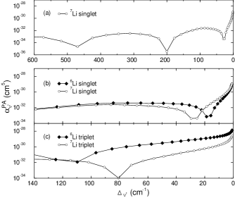
Figure 7: Variation of photoassociation rate coefficient $\alpha^{PA}_{v^{\prime}}$ for high-lying vibrational states. In (a), the ⁷Li singlet transitions over a range of 600 cm^-1 exhibit oscillations mapping the nodal structure of the continuum wave function, with values varying over five orders of magnitude. Plots (b) and (c) show a shorter range of detunings for singlet and triplet transitions, respectively. The singlet scattering lengths of both isotopes are positive and $\alpha^{PA}_{v^{\prime}}$ decays rapidly from its large values near $\Delta\sim 0$ cm^-1, by nearly three orders of magnitude. The triplet scattering lengths are both negative, and $\alpha^{PA}_{v^{\prime}}$ decreases slowly for small detunings, until the first nodes of the continuum wave functions are reached.

Much larger photoassociation rates and correspondingly smaller characteristic intensities can be obtained if the excited levels $v^{\prime}$ are closer to the dissociation limit (i.e., have smaller binding energies). In fact, the $v^{\prime}=58$ level is deeply bound, with a binding energy of $\hbar\Delta_{v^{\prime}=58}=5.5\times 10^{-4}$ hartree (or 122.22 cm^-1 note-hulet ). For example, $v^{\prime}=86$ with a binding energy of $0.87\,{\rm cm}^{-1}$ has a rate coefficient 1050 times larger, namely $\alpha^{PA}_{v^{\prime}=86}=2.1\times 10^{-29}$ cm⁵, which gives the characteristic intensity $I_{v^{\prime}=86}=0.032\,{\rm W\,cm^{-2}}$. The high-lying excited levels $v^{\prime}$ have larger rate coefficients because the overlap of the excited bound wave function and the continuum ground wave function is larger. For high $v^{\prime}$, the overlap scales like $\Delta_{v^{\prime}}^{-1/2}$.

Similar results for sodium and cesium are available. For small binding energies, the rate coefficient $\alpha^{PA}_{v^{\prime}}$ at 1 mK is of the order of $10^{-28}$ cm⁵ for Na, and $10^{-27}$ cm⁵ for Cs more-rates . These translate to characteristic intensities as small as $\rm\mu W\,cm^{-2}$. Notice that for lithium, the rate coefficients for singlet transitions are smaller than for triplet transitions, reflecting the sign of the scattering length: this is especially significant for ⁶Li, where the triplet scattering length is negative and enormous COT95a .

Other expressions based on semi-classical treatment have been developed pillet ; more-rates . For example, in pillet , the rate for $s$-wave contribution is

$${\cal R}_{v^{\prime}}\simeq\rho\lambda_{D}^{3}e^{-{\hbar\delta\over k_{B}T}}\sqrt{\frac{\pi^{2}}{{3\delta\Delta_{v^{\prime}}}}}\sin^{2}[k(R_{v^{\prime}}-A(k))]\kappa^{2};$$ (93)

where $\kappa={\bf d}\cdot{\bf E}/2\hbar$ is the Rabi frequency of the laser of intensity $I$, $A(k)$ represents a shift from the free solution, and $\Delta_{v^{\prime}}$ (again) is the detuning of the level $v^{\prime}$ from the dissociation limit. This expression is valid for $s$-wave scattering and at low detunings. In the limit $k\rightarrow 0$, $A(k_{R})\rightarrow a$, and the maximum of ${\cal R}_{v^{\prime}}$ is found to be at $\hbar\delta\simeq k_{B}T/2$, so that

$${\cal R}_{v^{\prime}}\simeq\rho\lambda_{D}^{3}e^{-1/2}\kappa^{2}\sqrt{\frac{2\pi^{2}\mu^{2}}{3\hbar^{3}\Delta_{v^{\prime}}}}\sqrt{k_{B}T}(R_{v^{\prime}}-a)^{2}\;.$$ (94)

This equation is similar to Eqs.(85)-(92). Notice that since $\lambda_{D}\propto 1/\sqrt{T}$, the rate scales as $1/T$ and $\Delta_{v^{\prime}}^{-1/2}$ for small detuning. For lithium at 0.140 mK (corresponding to the Doppler temperature), assuming a laser intensity of 1000 W/cm² (so that $\kappa=0.8\times 10^{10}$ s^-1: see pillet for details), and a detuning $\Delta_{v^{\prime}}\sim 1$ cm${}^{-1}\simeq 30$ GHz (or $4.5\times 10^{-6}$ hartree), we have $R_{v^{\prime}}=135\,a_{0}$ and $\lambda_{D}=1489\,a_{0}=7.875\times 10^{-6}$ cm. For a density $\rho=10^{11}$ cm^-3, this gives $\rho\lambda_{D}^{3}=4.88\times 10^{-5}$ and, neglecting the scattering length $a$, one gets ${\cal R}_{v^{\prime}}\sim 9.6\times 10^{4}$ s^-1. If we scale the rate to $T=1$ mK, we get $1.3\times 10^{4}$ s^-1, less than twice the value 7140 $s^{-1}$ obtained from Eq. (85) using the calculated value of $\alpha^{PA}_{v^{\prime}=86}$ given above. Notice that many assumptions are made in these estimates: nonetheless, expression (94) gives good order of magnitude for the photoassociation rate for small detuning and low temperatures.

Using the Doppler temperature as a typical temperature, and averaging the rate using a linewidth corresponding to 5 MHz pillet , one finds typical rates for small detunings by scaling the numbers of Table 2 with the appropriate temperature, density, laser intensity, and detunings, according to

$${{\cal R}_{v^{\prime}}}\simeq\frac{I}{I_{0}}\frac{\rho}{\rho_{0}}\frac{T_{0}}{T}\sqrt{\frac{\Delta_{0}}{\Delta_{v^{\prime}}}}\;\overline{\cal R}\;.$$ (95)

Here, $I_{0}=1000$ W/cm², $\rho_{0}=10^{11}$ cm^-3, $\Delta_{0}=1$ cm^-1, and $T_{0}$ and $\bar{\cal R}$ are listed in Table 2. Correspondingly, $\alpha^{PA}$ scales as

$$\alpha_{v^{\prime}}^{PA}\simeq\frac{T_{0}}{T}\sqrt{\frac{\Delta_{0}}{\Delta_{v^{\prime}}}}\;\overline{\alpha}^{PA}\;.$$ (96)

The characteristic intensities should then scale with the square root of the detuning $\Delta_{v^{\prime}}$, so that we have

$$I_{v^{\prime}}=\sqrt{\frac{\Delta_{v^{\prime}}}{\Delta_{0}}}\,I_{0}\,.$$ (97)

Table 2: Approximate scaled photoabsorption rates $\overline{\cal R}$ and rate coefficients $\overline{\alpha}^{PA}$ for weakly bound molecular states. The values of $\overline{\cal R}$, and $T_{0}$ are from Pillet et al. pillet , $I_{0}=1000$ W cm^-2, $\rho_{0}=10^{11}$ cm ^-3, and $\Delta_{0}=1$ cm^-1.

Atom	$T_{0}$	$\overline{\cal R}$	$\lambda$	$\varphi$	$\overline{\alpha}^{PA}$
	mK	$10^{4}$ s-1	nm	$10^{21}$ cm-2	cm5
Li	0.140	45	671	3.4	$1.3\times 10^{-27}$
Na	0.240	22	589	3.0	$7.3\times 10^{-28}$
K	0.140	25	766	3.9	$6.6\times 10^{-28}$
Rb	0.140	13	780	3.9	$3.3\times 10^{-28}$
Cs	0.125	10	852	4.3	$2.3\times 10^{-28}$

The values of $\lambda$, $\varphi$ and $\overline{\alpha}^{PA}$ are listed in Table 2. To compare the rates for the various alkali metals, it is convenient to express them for the same parameters. Assuming $I_{0}=1000$ W/cm², $\rho=10^{11}$ cm^-3, $T=100$ $\mu$K, and $\Delta_{0}=1$ cm^-1, we obtain the values listed in Table 3. The photoassociation rates vary between $1.2\times 10^{5}$ s^-1 (or $\alpha^{PA}\sim 2.9\times 10^{-28}$ cm⁵) for Cs and $6.3\times 10^{5}$ s^-1 (or $\alpha^{PA}\sim 1.8\times 10^{-27}$ cm⁵) for Li. From the expressions for ${\cal R}_{v^{\prime}}$, one expects the rates to scale like $1/2\mu$. If we were to multiply the rates by $M$, the mass number, we notice that, except for Li, the scaled rates indeed are similar. The variations left are due to slightly different Rabi frequencies pillet .

Table 3: Approximate photoassociation rates $\cal R$, rate coefficients $\alpha^{PA}$, and characteristic intensities $I_{v^{\prime}}$ for the alkalis. The fixed parameters are $I_{0}=1000$ W/cm², $\rho_{0}=10^{11}$ cm^-3, $\Delta_{0}=1$ cm^-1, and T=100 $\mu$K,. Also listed are the reference densities $\lambdabar^{-3}$ (in cm^-3) and frequencies $\epsilon_{R}$ (in $2\pi\,{\rm kHz}$).

Atom	${\cal R}_{v^{\prime}}$	$\alpha^{PA}_{v^{\prime}}$	$I_{v^{\prime}}$	$\lambdabar^{-3}$	$\epsilon_{R}$
	$10^{4}$s-1	cm5	${\rm mW\,cm}$-2	cm-3	$2\pi\,{\rm kHz}$
7Li	63	$1.8\times 10^{-27}$	3.7	$8.21\times 10^{14}$	63.3
23Na	53	$1.7\times 10^{-27}$	0.47	$1.21\times 10^{15}$	25.0
39K	35	$9.2\times 10^{-28}$	0.18	$5.52\times 10^{14}$	8.72
87Rb	18	$4.6\times 10^{-28}$	0.069	$5.23\times 10^{14}$	3.77
133Cs	12	$2.9\times 10^{-28}$	0.039	$4.01\times 10^{14}$	2.07

Finally, one has to be careful when using the values of Table 3, in which the effect of scattering lengths are not taken into account. These effects can be significant, like in the case of ⁶Li, ⁸⁵Rb or ¹³³Cs, where large negative scattering lengths induce larger rates. Also, at larger detunings, one probes deeper region of the excited electronic state, and shorter distances of the lower state continuum wave function, where the exact nodal structure will play an important role (see COT95 ; cote-pra ; cote-jms and Fig. 7).

As already noted, the values for the saturation intensity in Table 3 are to be construed as estimates only. Also, as they are, they apply to a very weakly bound molecular state ($\Delta_{v^{\prime}}=1~{}{\rm cm}^{-1}$). Such high-lying states are likely to be easily perturbed by atom-molecule collisions, so that in practice one might resort to more bound molecular states. Nonetheless, these saturation intensities are remarkably low, occasionally much lower than our initial generic estimate of $10\,{\rm Wcm}^{-2}$ JAV99 ; JAV99a . From the experimental viewpoint this is encouraging, as the requirements on laser intensity are greatly moderated. The flip side is that the usable intensity appears to be limited by rogue photoassociation; for densities such that $\lambdabar^{3}\rho\sim 1$, the maximum photoassociation Rabi frequency is of the order of the recoil frequency $\epsilon_{R}$ . For heavier alkalis the saturation intensities may indeed be low, but small recoil frequency and slow coherent photoassociation are the prices to pay.

V.4 Discussion of an experiment

In the experiment of Wynar et al., Ref. WYN00 , the authors studied photoassociation of a ⁸⁷Rb condensate in a two-color Raman configuration. From our standpoint, the reported data fall into two categories. First, the width and shift of the two-photon resonance line was studied as a function of the intensities of the two lasers. We are going to use these measurements to estimate the bound-bound Rabi frequency. Second, the authors measured the width and the shift of the same resonance line as a function of the density of the condensate. At low intensities, elastic atom-atom and atom-molecule collisions turn out to have a major effect on the resonance parameters. However, these effects were modeled quantitatively in Ref. WYN00 , and one may then get at the quantities pertaining to photoassociation. We use this type of data to determine the characteristic frequency of coherent photoassociation.

V.4.1 Adapting the theory

We first cast our theoretical approach in a form that allows for direct juxtapositions with the analysis of experimental data in Ref. WYN00 . We ignore elastic collisions because a comparison with Ref. WYN00 turns out to be possible even without considering them explicitly, and inelastic collisions because their presence was not conclusively established in Ref. WYN00 .

We begin by adding the spontaneous decay of the intermediate state at the rate $\Gamma_{s}$ as a nonhermitian term in the Hamiltonian for the $\Lambda$ system, Eq. (72). This gives

$${H\over\hbar}=\delta\,g^{\dagger}g+(\Delta+\delta)b^{\dagger}b+\ldots-i{\Gamma_{s}\over 2}\,b^{\dagger}b\,.$$ (98)

It is known in quantum optics that introducing an imaginary part to the energy of the decaying state gives correct results as long as the unstable state decays irreversibly only to states that are outside of the state space included in the model.

We then repeat much of the analysis of Sec. V.2.1 for the Hamiltonian (98), with a number of tricks and approximations. First, we take the limit of large intermediate detuning, $|\Delta|\gg\Gamma_{s},|\delta|$. Second, we assume that the bound-bound Rabi frequency $\chi$ is much larger than the free-bound Rabi frequency $\Omega$. This implies that in the estimates of the line widths and decay rates, such as those following from Eq. (81), only the $\chi^{2}$ terms need be kept. Third, we ignore light-induced atom-atom interactions. Fourth, we scale the the operators as before, $a=\sqrt{N}\alpha$, etc., which brings out the photoassociation frequency $\Omega$ explicitly. Fifth, after deriving the equations of motion for the atomic operator $\alpha$ and final-state molecule operator $\gamma$ by adiabatic elimination of the intermediate-state operate $\beta$, in the spirit of semiclassical approximation we replace the operators $\alpha$, $\beta$, and $\gamma$ with $c$ numbers. At this stage we have, in analogy with Eqs. (77) and (78), the equations

$$\dot{\gamma} = -i\left(\delta-{\chi^{2}\over\Delta}\right)\gamma-{\Gamma_{s}\chi^{2}\over 2\Delta^{2}}\,\gamma+\hbox{$1\over 2$}i\,{\Omega\chi\over\Delta}\,\alpha^{2},$$ (99)

$$\dot{\alpha} = i\,{\Omega\chi\over\Delta}\alpha^{*}\gamma\,.$$ (100)

To develop the rate approximation, we first note that the probability that an atom belongs to the stable state $g$, $P_{g}=2|\gamma|^{2}$, satisfies the equation of motion

$$\dot{P}_{g}=-{\Gamma_{s}\chi^{2}\over\Delta^{2}}\,P_{g}+i{\Omega\chi\over\Delta}(C-C^{*})\,.$$ (101)

The “coherence” $C=\alpha^{2}\gamma^{*}$ has the equation of motion

$$\dot{C}=i{\Omega\chi\over\Delta}[P_{g}P_{a}-\hbox{$1\over 2$}P_{a}^{2}]+\left[i\left(\delta-{\chi^{2}\over\Delta}\right)-{\Gamma_{s}\chi^{2}\over 2\Delta^{2}}\right]C\,,$$ (102)

where, in turn $P_{a}=|\alpha|^{2}$ is the probability that an atom remains in the system unassociated.

We could go on and derive a corresponding equation of motion for $P_{a}$. However, here we assume that $P_{a}\sim 1$, and that correspondingly $P_{g}\ll 1$. We solve for the coherence $C$ adiabatically by setting $\dot{C}=0$, and insert the result into Eq. (101) to obtain a rate equation for the population of the stable molecular state $g$,

$$\dot{P}_{g}=-{\Gamma_{s}\chi^{2}\over\Delta^{2}}\,P_{g}+{\left[{\Omega\chi\over\Delta}\right]^{2}\left[{\Gamma_{s}\chi^{2}\over 2\Delta^{2}}\right]\over\left[\delta-{{\chi^{2}\over\Delta}}\right]^{2}+\left[{\Gamma_{s}\chi^{2}\over 2\Delta^{2}}\right]^{2}}\,P_{a}^{2}\,.$$ (103)

This displays a shift of the ground state by

$$\Delta\varepsilon_{L}={\chi^{2}\over\Delta}\,,$$ (104)

a linewidth

$${\gamma_{L}\over 2}={\Gamma_{s}\chi^{2}\over 2\Delta^{2}}\,,$$ (105)

and a corresponding direct decay of bound molecules at the rate $\gamma_{L}$.

With the assumption $P_{g}\ll 1$ we have made the rate equation (103) essentially one way, i.e., ignored transitions from molecules back to the atoms. The semiclassical approximation in general requires that there are many molecules in a quantum state, so that the molecules make a condensate. However, we believe that, by ignoring transitions from molecules back to atoms, we have divorced the rate equation (103) from any coherence requirement for the molecules. As the experiments do not claim a molecular condensate, this is essential for the analysis that follows.

V.4.2 Comparison with experiments

Wynar et al., Ref. WYN00 , discuss the light shift of the resonance line. In their case the frequencies of the two lasers are quite close so that both of them cause line shifts and broadenings, but this is included in their analysis. Translating back to our case with only one laser frequency on the bound-bound transition, the comparison between our formulation and Ref. WYN00 reads

$${\chi^{2}\over\Delta}={\beta I_{2}\over\Delta_{1}}\,,$$ (106)

where $I_{2}$ is the intensity (in W cm^-2) of the bound-bound light, $\Delta_{1}\equiv\Delta=2\pi\times 150\,{\rm MHz}$ is the intermediate detuning, and $\beta=3.5\times 10^{9}\,{\rm m^{2}W^{-1}s^{-2}}$ is a parameter that we deduce from their Fig. 3a. This gives the approximate formula

$$\chi\simeq 0.94\,\sqrt{I_{2}\over{\rm Wcm^{-2}}}\times 2\pi\,{\rm MHz}\,.$$ (107)

Wynar et al., Ref. WYN00 , also present an analysis of line shapes at low intensity. The rate coefficient for two-photon photoassociation on resonance, $K_{0}=9\times 10^{-14}\,{\rm cm^{3}\,s^{-1}}$, is one of the fitted parameters. The resonance photoassociation rate from our Eq. (103) and the corresponding expression in Ref. WYN00 , ignoring inelastic processes and with $n\equiv\rho$, boil down to

$${\Omega^{2}\over\Gamma_{s}}={nK_{0}}\,.$$ (108)

Given the spontaneous decay rate of this molecular level, $\Gamma_{s}=12\times 2\pi\,{\rm MHz}$ WYN00 , and noting that their cited value of $K_{0}$ was for the intensity of the photoassociation laser $I_{1}=0.51\,{\rm W\,cm^{-2}}$, we find the scaling formula

$$\Omega\simeq 5.8\,\sqrt{{\rho\over 10^{14}{\rm cm^{-3}}}\,{I_{1}\over{\rm Wcm^{-2}}}}\,\times 2\pi\,{\rm kHz}\,,$$ (109)

which gives the characteristic intensity $I_{v^{\prime}}=0.08\,{\rm Wcm^{-2}}$.

In the experiment, the binding energy of the primary photoassociated state was 23 cm^-1. In contrast, for $\Delta_{v^{\prime}}=1\,{\rm cm}^{-1}$, Table 3 gives the characteristic intensity $0.07\,{\rm mWcm^{-2}}$. The theoretical and experimental characteristic intensities differ by three orders of magnitude, but they are also for different binding energies. The difference in characteristics intensities is no cause for concern, as we do not know at all how the detuning 23 cm^-1 for Rb is related to the minima of the photoassociation rates like those shown in Fig. 7 for Li.

V.4.3 Reaching coherence

Suppose that the density of the ⁸⁷Rb gas equals $\rho=\lambdabar^{-3}$, a factor of two larger than quoted in Ref. WYN00 , the laser intensities are $I_{1}=I_{2}=10\,{\rm W\,cm^{-2}}$, typical values in photoassociation experiments, and the intermediate detuning is as in Ref. WYN00 . Then the two-photon Rabi frequency becomes $\Omega\chi/\Delta=1\,\times 2\pi\,{\rm kHz}$, while the effective linewidth is $\chi^{2}\Gamma_{s}/2\Delta^{2}=2\times 2\pi\,{\rm kHz}$. For coherent phenomena we need a Rabi frequency at least comparable to the linewidth, a condition that is not quite satisfied. But if one were simply to take the intensities $I_{1}=100\,{\rm W\,cm^{-2}}$ for the photoassociating light and $I_{2}=1\,{\rm W\,cm^{-2}}$ for the bound-bound light, Rabi frequency remains unchanged and linewidth goes down by a factor of 100. One is then in principle deep in the regime of coherent photoassociation. Also, the effective Rabi frequency would be smaller than the recoil frequency, so that rogue photoassociation need not yet be a fatal problem.

On the other hand, eyeballing from Fig. 2 of Ref WYN00 , the linewidth due to elastic atom-atom collisions would be of the order of $5\times 2\pi\,{\rm kHz}$, so elastic collisions would interfere with coherent photoassociation. Rabi oscillations would be seriously impeded, rapid adiabatic passage maybe less. One could compensate by lowering the density by two orders of magnitude and at the same time increasing the intensity of the photoassociating laser by another two orders of magnitude to keep the effective Rabi frequency constant, but with lowering of the density one would wind up in trouble with rogue photoassociation.

Experimentally, one can think of varying the intensity of the two lasers, the intermediate state, the intermediate detuning, and the density of the sample. The conditions one must watch out for are that effective Rabi frequency be larger than the effective damping rate and line broadening due to elastic (and inelastic) collisions, yet not so large as to cause excessive rogue photoassociation. If the parameters could be varied freely, within our physical model a solution is always possible. Unfortunately, one must live with some practical limitations on, say, laser intensities. The present experiment of Ref. WYN00 is tantalizingly close to coherent photoassociation, but to really get there may require a careful optimization of the experimental parameters and a solid understanding of what is technically feasible in a given experiment. We will not attempt to enter such discussions.

VI Concluding remarks

We have developed theory for coherent photoassociation of a Bose-Einstein condensate of atoms, which typically leads to a Bose-Einstein condensate of molecules. Phenomena analogous to coherent optical transients in few-level systems, such as Rabi flopping and rapid adiabatic passage between atomic and molecular condensates are expected. Coherent phenomena depend on the Bose enhancement of the dipole moment matrix element, and cannot occur in a nondegenerate gas, at least not in the thermodynamic limit. Bose-Einstein condensation and photoassociation are both currently front-line research and the marriage thereof might still be a technological challenge, but coherent optical transients in photoassociation should eventually be feasible in experiments.

Appendix A Dipole matrix element

In our bare-bones example we consider the situation in which we either have one molecule at rest and no atoms, or no molecule and two atoms in states ${\bf k}$ and $-{\bf k}$. Then the relative momentum becomes $\hbar{\bf k}$. This peculiarity, and also the reason for the factor $1\over 2$ in Eq. (14), is because the relative momentum for two entities with momenta ${\bf p}_{1}$ and ${\bf p}_{2}$ should be defined as $\hbox{$1\over 2$}({\bf p}_{1}-{\bf p}_{2})$ to make it the conjugate of the usual relative position ${\bf r}_{1}-{\bf r}_{2}$. We thus have the possible state vectors

$$|\psi\rangle=\left(\beta\,b^{\dagger}+\sum_{\bf k}\alpha_{\bf k}a^{\dagger}_{\bf k}a^{\dagger}_{-{\bf k}}\right)|0\rangle\,,$$ (110)

where $\beta$ and $\alpha_{k}$ are complex amplitudes to be determined, and $|0\rangle$ stands for the vacuum of atoms and molecules. The states for $\alpha_{\bf k}$ and $\alpha_{-{\bf k}}$ are the same, so the sum over ${\bf k}$ runs only over half of the possible ${\bf k}$ values; say, those with $k_{x}>0$.

Following Ref. JAV99 , we write the time dependent Schrödinger equation from the Hamiltonian (12) in terms of the coefficients $\beta$ and $\alpha_{k}$, assuming a plane wave of light. In order to avoid an inessential complication, we ignore photon recoil and simply set ${\bf q}=0$. The result is

$$\dot{\alpha}_{\bf k} = -i\left({\hbar{\bf k}^{2}\over 2\mu}-\delta_{0}\right)\alpha_{\bf k}+i{{\bf d}^{*}\cdot{\bf E}^{*}\over 2\hbar}\,\beta,$$ (111)

$$\dot{\beta} = i\sum_{\bf k}{{\bf d}\cdot{\bf E}\over 2\hbar}\,\alpha_{\bf k}\,.$$ (112)

The QC approach discussed in Refs. JAV98 and MAC99 displays precisely the same structure, evidently identifying ${\bf d}\cdot{\bf E}/2\hbar$ as the QC Rabi frequency $\kappa$ of those papers.

There is a catch, however. Because of the Bose-Einstein statistics, states with the relative momenta for two atoms ${\bf k}$ and $-{\bf k}$ are the same, so the density of states for the relative motion is half of what it was for Maxwell-Boltzmann atoms. To obtain the same photodissociation rate, we therefore have to make the matrix element a factor of $\sqrt{2}$ larger than in the case of distinguishable atoms. This is the $\sqrt{2}$ in Eq. (14). The rate of photodissociation is proportional to the square of the matrix element and picks up a factor of two, which compensates for the missing half of phase space density.

The second-quantized Hamiltonian is chosen so that it gives the right photodissociation rate. What we did not fully realize in Ref. JAV99 is that the same factor of $\sqrt{2}$ also leads to twice the photoassociation rate that one would obtain for Maxwell-Boltzmann atoms, given the Franck-Condon factor from the standard calculations or as deduced from the photodissociation rate. It appears that in the literature the rate for $s$-wave photoassociation is usually calculated low by a factor of two. Besides, by a simple extension of the statistics arguments, $p$-wave photoassociation should vanish for bosons. Are these problems?

We think not. In photoassociation experiments no particular care is usually taken to polarize the atoms. They are not all in the same internal state, and therefore not all photoassociation events are between indistinguishable atoms. This should reduce the factor-of-two boson enhancement of the photoassociation rate for even partial waves, and call forth odd partial waves. The remaining discrepancies with the conventional calculations may well be within experimental and theoretical uncertainties.

It would be of some interest to investigate photoassociation of a polarized low-temperature gas experimentally. We believe that the statistics effects are real, and should be observable. After all, few colleagues seem to have a problem with the assertion that there are no $s$-wave collisions for polarized fermions. Photoassociation experiments in a polarized gas should make an interesting test of our phenomenological Hamiltonian.

Appendix B Kernel for photoassociation in field theory

The process we followed in the main text in deriving the integral kernel ${\bf d}({\bf r})$ [as in, e.g., Eq. (23)] was a phenomenological mix between formally pure field theory and collisional physics.

In fact, to obtain the dipole matrix elements ${\bf d}_{{\bf k}{\bf k}^{\prime}}$ in Eq. (12), we carry out an integral of the form

$${\bf d}_{{\bf k}{\bf k}^{\prime}}\equiv{\bf d}({\bf k}-{\bf k}^{\prime})={\bf d}\int d^{3}r\,\bar{\psi}^{*}({\bf r})\bar{\phi}_{{\bf k}-{\bf k}^{\prime}}({\bf r})\,,$$ (113)

where $\bar{\psi}$ is the bound-state molecular wave function and $\bar{\phi}_{{\bf k}-{\bf k}^{\prime}}$ describes the state of two atoms with the relative momentum $\hbar({\bf k}-{\bf k}^{\prime})$. Now, in the transformation to field theory (18) we used plane waves as the wave functions for states with a given wave vector. In the matrix element (113) we should correspondingly use plane waves to describe the relative motion, as in

$$\bar{\phi}_{{\bf k}-{\bf k}^{\prime}}({\bf r})={1\over\sqrt{V}}\,e^{i({\bf k}-{\bf k}^{\prime})\cdot{\bf r}}\,.$$ (114)

However, in our derivation we did not not use plane waves, but distorted plane waves that take into account atom-atom interactions, and only asymptotically (at large distances) corresponds to the relative momentum ${\bf k}-{\bf k}^{\prime}$.

This makes a difference. For instance, if the matrix element (113) is computed using pure plane waves, the final photoassociation kernel reads

$${\bf d}({\bf r})=\sqrt{2}\,{\bf d}\,\bar{\psi}^{*}(r)\,,$$ (115)

instead of something akin to (LABEL:DR1). Depending on the value of the scattering length, there could be a substantial difference in the overall numerical factor also in the contact-interaction form for atom-molecule coupling, Eq. (24). The question is, which method is “correct”; pure or distorted plane waves?

First of all, atoms do interact, which in general will have an effect on photoassociation. One who wishes to analyze photoassociation quantitatively will have to take atom-atom interactions into account. A field theorist pursuing pure plane waves would have to consider atom-atom interactions explicitly, and work out the consequences in photoassociation ab initio. This is probably a major chore. Our hope is that, with our distorted-plane wave trickery, we have phenomenologically captured most of the effect of atom-atom interactions on photoassociation.

On the other hand, if we use the distorted plane waves to calculate the photoassociation matrix element and in addition introduce a contact interaction model for atoms as in (83), the suspicion arises that we are double-counting atom-atom interactions. Further approximations, such as the contact-interaction form for photoassociation or classical field theory, could either exacerbate or ameliorate the double-counting.

Disentangling atom-atom interactions and photoassociation might make an interesting theoretical exercise, but we do not attempt it in this paper. Instead, we proceed with a model that allows for both distorted-plane wave matrix elements for photoassociation, and an explicit atom-atom interaction. In this way, we at least get the limiting cases of photoassociation in a dilute gas and atom-atom interactions in the absence of photoassociation basically right with little effor

References

- (1) H. R. Thorsheim, J. Weiner, and P. S. Julienne, Phys. Rev. Lett. 58, 2420 (1987); R. Napolitano, J. Weiner, C. J. Williams, and P. S. Julienne, Phys. Rev. Lett. 73, 1352 (1994); P. D. Lett, P. S. Julienne, and W. D. Phillips, Annu. Rev. Phys. Chem. 46, 423 (1995).
- (2) M. H. Anderson, J. R. Ensher, M. R. Matthews, C. E. Wieman, and E. A. Cornell, Science 269, 198 (1995); K. B. Davis, M. -O. Mewes, M. R. Andrews, N. J. van Druten, D. S. Durfee, D. M. Kurn, and W. Ketterle, Phys. Rev. Lett. 75, 3969 (1995); C. C. Bradley, C. A. Sackett, and R. G. Hulet, Phys. Rev. Lett. 78, 985 (1997).
- (3) E. R. I. Abraham, W. I. McAlexander, C. A. Sacket, and R. G. Hulet, Phys. Rev. Lett. 74, 1315 (1995); E. Tiesinga, C. J. Williams, P. S. Julienne, K. M. Jones, P. D. Lett, and W. D. Phillips, J. Res. Natl. Inst. Stand. Technol. 101, 505 (1996); C. C. Tsai, R. S. Freeland, J. M. Vogels, H. M. J. M. Boestan, B. J. Verhaar, and D. J. Heinzen, Phys. Rev. Lett. 79, 1245 (1997).
- (4) K. Burnett, P. S. Julienne, and K.-A. Suominen, Phys. Rev. Lett. 77, 1416 (1997).
- (5) P. S. Julienne, K. Burnett, Y. B. Band, and W. C. Stwalley, Phys. Rev. A 58, R797 (1998).
- (6) J. Javanainen and M. Mackie, Phys. Rev. A 58, R789 (1998).
- (7) M. Mackie and J. Javanainen, Phys. Rev. A 60, 3174 (1999).
- (8) J. Javanainen and M. Mackie, Phys. Rev. A 59, R3186 (1999).
- (9) P. D. Drummond, K. V. Kheruntsyan, and H. He, Phys. Rev. Lett. 81, 3055 (1998).
- (10) P. Tommasini, E. Timmermans, M. Hussein, and A. Kerman; LANL preprint archive cond-mat/9804015.
- (11) E. Timmermans, P. Tommasini, R. Côté, M. Hussein, and A. Kerman, Phys. Rev. Lett. 83, 2691 (1999).
- (12) F. A. van Abeelen and B. J. Verhaar, Phys. Rev. Lett. 83, 1550 (1999).
- (13) M. Mackie, R. Kowalski, and J. Javanainen, Phys. Rev. Lett. 84, 3803 (2000).
- (14) J. Javanainen and M. Kos̆trun, Optics Express 5, 188 (1999).
- (15) M. Mackie and J. Javanainen, J. Mod. Opt. xx, yyyy (2000).
- (16) R. Wynar, R. S. Freeland, D. J. Han, C. Ryu, and D. J. Heinzen, Science 287, 1016 (2000).
- (17) R. Côté, A. Dalgarno, Y. Sun, and R. G. Hulet, Phys. Rev. Lett. 74, 3581 (1995)
- (18) E. R. I. Abraham, W. I. McAlexander, J. M. Gerton, R. G. Hulet, R. Côté, and A. Dalgarno, Phys. Rev. A 53, R3173 (1996).
- (19) The “well-known” universality of the mode density, independently of the shape of the quantization volume, goes back at least to the work of Hermann Weyl in the beginning of the 20th century. See Selecta Hermann Weyl (Birkhäuser, Basel, 1956), pp. 59–110.
- (20) J. Javanainen and M. Ivanov, Phys. Rev. A 60, 2351 (1999).
- (21) D. F. Walls and C. T. Tindle, J. Phys. A 5, 534 (1972).
- (22) G. Drobny and I. Jex, Phys. Rev. A 45, 1816 (1992).
- (23) H. He, M. J. Werner, and P. D. Drummond, Phys. Rev. E 54, 896 (1996).
- (24) S. Wolfram, The Mathematica Book, 3rd Ed. (Cambridge University Press, New York, 1996).
- (25) S. Trillo and P. Ferro, Optics Lett. 20, 438 (1995).
- (26) H. He, P. D. Drummond, and B. A. Malomed, Optics. Comm. 123 (1996).
- (27) M. D. Fleck and J. A. Feit, J. Chem. Phys. 78, 2578 (1984); A. D. Bandrauk and H. Shen, Can. J. Chem. 70, 555 (1992).
- (28) D. V. Skryabin and W. J. Firth, Optics Comm. 148, 79 (1998).
- (29) K. Rzazewski, M. Lewenstein, and J. H. Eberly, J. Phys. B 15, L661 (1982).
- (30) D. Heinzen and W. Ketterle (unpublished) have developed the estimate (71) from completely different arguments.
- (31) P. O. Fedichev, Yu. Kagan, G. V. Shlyapnikov, and J. T. M. Walraven, Phys. Rev. Lett. 77, 2913 (1996).
- (32) J. L. Bohn and P. S. Julienne, Phys. Rev. A 54, R4637 (1996).
- (33) J. L. Bohn and P. S. Julienne, Phys. Rev. A 60, 414 (1999).
- (34) J. Javanainen, J. Phys. B 16, 1343 (1983); Optics Commun. 46, 175 (1983); Physica Scripta 31, 57 (1985).
- (35) See J. Weiner, V.S. Bagnato, S. Zilio, and P.S. Julienne, Rev. Mod. Phys. 71, 1 (1999), and references therein.
- (36) R. Côté and A. Dalgarno, Phys. Rev. A 58, 498 (1998).
- (37) R. Côté and A. Dalgarno, J. Mol. Spect. 195, 236 (1999).
- (38) The rate coefficients listed in Refs. cote-pra ; cote-jms must be multiplied by , and we do not assume any hyperfine mixing (neglect in cote-pra ; cote-jms ).
- (39) We determined the binding energy of level of 7Li triplet state to be GHz by fitting the known levels, and it was recently measured by R.G. Hulet and co-workers to be 3667 GHz.
- (40) P.S. Julienne, J. Res. Natl. Stand. Technol. 101, 487 (1996); F. Masnou-Seeuws, O. Dulieu, A. Crubellier, and P. Pillet (private communication).
- (41) P. Pillet, A. Crubellier, A. Bleton, O. Dulieu, P. Nosbaum, I. Mourachko, and F. Masnou-Seeuws, J. Phys. B 30, 2801 (1997).