FINITE-DIFFERENCE CALCULATIONS FOR ATOMS AND DIATOMIC MOLECULES IN STRONG MAGNETIC AND STATIC ELECTRIC FIELDS

Abstract

Fully numerical mesh solutions of 2D quantum equations of Schrödinger and Hartree-Fock type allow us to work with wavefunctions which possess a very flexible geometry. This flexibility is especially important for calculations of atoms and molecules in strong external fields where neither the external field nor the internal interactions can be considered as a perturbation. The applications of the present approach include calculations of atoms and diatomic molecules in strong static electric and magnetic fields. For the latter we have carried out Hartree-Fock calculations for He, Li, C and several other atoms. This yields in particular the first comprehensive investigation of the ground state configurations of the Li and C atoms in the whole range of magnetic fields ($0<B<10000$ a.u.) and a study of the ground state electronic configurations of all the atoms with $1<Z\leq 10$ and their ions ${\rm A^{+}}$ in the high-field fully spin-polarised regime. The results in a case of a strong electric field relate to single-electron systems including the correct solution of the Schrödinger equation for the ${\rm H_{2}^{+}}$ ion (energies and decay rates) and the hydrogen atom in strong parallel electric and magnetic fields.

I Introduction

Theoretical studies of atoms and molecules in strong external fields are motivated by several applications. The latter are e.g. experiments with intense laser beams (electromagnetic fields with dominating electric component) and astronomical observations of white dwarfs and neutron stars (magnetic fields). The experimental availability of extremely strong electric fields in laser beams makes the theoretical study of various atomic and molecular species under such conditions very desirable. The properties of atomic and molecular systems in strong fields undergo dramatic changes in comparison with the field-free case. These changes are associated with the strong distortions of the spatial distributions of the electronic density and correspondingly the geometry of the electronic wavefunctions. This complex geometry is difficult for its description by means of traditional sets of basis functions and requires more flexible approaches which can, in particular, be provided by multi-dimensional mesh finite-difference methods.

Let us discuss the problem of atoms in a strong magnetic field in more detail. We start this consideration with the hydrogen atom which was the first atom whose behaviour in strong magnetic fields was investigated (for a list of references see Fri89 ; RWHR ; Ivanov88 ; Kra96 ). In cylindrical coordinates $(\rho,z)$ its non-relativistic Hamiltonian has the form (we use atomic units throughout our work)

$$H=-\frac{1}{2}\left(\frac{\partial^{2}}{\partial\rho^{2}}+\frac{1}{\rho}\frac{\partial}{\partial\rho}+\frac{\partial^{2}}{\partial z^{2}}-\frac{m^{2}}{\rho^{2}}\right)+s_{z}\gamma+\frac{m}{2}\gamma+\frac{\gamma^{2}}{8}\rho^{2}-\frac{1}{r}$$ (1)

where $m$ is the magnetic quantum number, $s_{z}$ is the spin $z$ projection and $\gamma=B/B_{0}$, $B_{0}=\hbar c/ea_{0}^{2}=2.3505{\cdot}10^{5}$T is the magnetic field strength in atomic units. The magnetic field is parallel to the $z$ axis. The Hamiltonian (1) contains two potentials of different spatial symmetries: the spherical-symmetric Coulomb term $1/r$ and the cylindrically symmetric potential of the magnetic field $\gamma^{2}\rho^{2}/8$. When considering the impact of the competing Coulomb and diamagnetic interaction it is reasonable to distinguish the three different regimes of weak, strong and intermediate fields. In the latter case the magnetic and Coulomb forces are comparable. In the case of relatively weak fields the main features of the geometry of the wavefunction are determined by the dominating Coulomb term whereas the effect of the magnetic field can be consider as a perturbation of the Coulomb wavefunctions. For the opposite situation of very strong magnetic fields and dominating cylindrical symmetry the adiabatic approximation ElLoudon ; Neuhauser ; Godefroid was the main theoretical tool during the last four decades. This approximation separately considers the fast motion of the electron across the field and its slow motion in a modified Coulomb potential along the field direction. Both early (see Garstang ) and more recent works RWHR ; SimVir78 ; Friedrich ; Fonte ; Schmidt on the hydrogen atom have used different approaches for these regimes of the magnetic field. All these calculations had problems when considering the hydrogen atom in fields of intermediate strength. The detailed calculations of the hydrogen energy levels carried out by Rösner et al RWHR also retained the separation into different regimes of the field strength by decomposing the electronic wave function either in terms of spherical (weak to intermediate fields) or cylindrical (intermediate to high fields) orbitals. A solution allowing to obtain comprehensive results on low-lying energy levels of the hydrogen atom for arbitrary field strengths including the intermediate field regime is provided by the multi-dimensional mesh solution of the Schrödinger equation Ivanov88 .

For different electronic degrees of excitation of the atom the intermediate regime is met for different absolute values of the field strength. For the ground state this regime is roughly given by $\gamma=~{}0.2-20$. For atoms with several electrons there are two decisive factors which enrich the possible changes in the electronic structure with varying field strength compared to the one-electron system. First, we have a third competing interaction which is the electron-electron repulsion and, second, the different electrons feel very different Coulomb forces, i.e. possess different one particle energies, and consequently the regime of the intermediate field strengths appears to be the sum of the intermediate regimes for the separate electrons.

The fact that most methods have problems in the intermediate field region has consequences for the current state of the art of our knowledge on on multi-electron atoms in strong magnetic fields. There exist a number of such investigations in the literature Neuhauser ; Godefroid ; Mueller75 ; Virtamo76 ; Larsen ; Gadiyak ; VinBay89 ; Ivanov91 ; TKBHRW ; Ivanov94 ; JonesOrtiz ; JonesOrtiz97 . The majority of them deals with the adiabatic regime in superstrong fields and the early works are mostly Hartree-Fock (HF) type calculations. There are also several early variational calculations for the low-field domain Larsen ; Henry74 ; Surmelian74 . HF calculations for arbitrary field strengths have been carried out in refs.RWHR ; TKBHRW by applying two different sets of basis functions in the high- and low-field regimes. As a result of the complicated geometry this approach suffers in the intermediate regime from very slow convergence and low accuracy of the calculated energy eigenvalues. Accurate HF calculations for arbitrary field strengths were carried out in refs. Ivanov91 ; Ivanov94 by the 2D mesh HF method. Investigations on the ground state as well as a number of excited states of helium including the correlation energy have recently been performed via a Quantum Monte Carlo approach JonesOrtiz97 . Very recently benchmark results with a precision of $10^{-4}-10^{-6}$ for the energy levels have been obtained for a large number of excited states with different symmetries using a configuration interaction approach with an anisotropic Gaussian basis set Bec99 ; Bec2000 . Focusing on systems with more than two electrons however the number of investigations is very scarce Neuhauser ; JonesOrtiz ; Muell84 . In view of the above there is a need for further quantum mechanical investigations and for data on atoms with more than two electrons in a strong magnetic field. For the carbon atom there exist two investigations Neuhauser ; Godefroid in the adiabatic approximation which give a few values for the binding energies in the high field regime and one more relevant recent work by Jones et al JonesOrtiz . On the other hand, our two-dimensional Hartree-Fock approach allowed us recently to perform precise and reliable consideration of a series of multi-electron atoms for the whole range of the magnetic field strengths from $\gamma=0$ up to ultrastrong fields $\gamma=10^{3}-10^{4}$ Ivanov91 ; Ivanov94 ; Ivanov98 ; IvaSchm98 ; IvaSchm99 ; IvaSchm2000 .

II Two-dimensional mesh Hartree-Fock method

Our calculations for multi-electron atoms in magnetic fields are carried out under the assumption of an infinitely heavy nucleus in the (unrestricted) Hartree-Fock approximation. The solution is established in the cylindrical coordinate system $(\rho,\phi,z)$ with the $z$-axis oriented along the magnetic field. We prescribe to each electron a definite value of the magnetic quantum number $m_{\mu}$. Each single-electron wave function $\Psi_{\mu}$ depends on the variables $\phi$ and $(\rho,z)$

$$\Psi_{\mu}(\rho,\phi,z)=(2\pi)^{-1/2}e^{-im_{\mu}\phi}\psi_{\mu}(z,\rho)$$ (2)

where $\mu$ denotes the numbering of the electrons. The resulting partial differential equations for $\psi_{\mu}(z,\rho)$ have been presented in ref.Ivanov94 .

The one-particle equations for the wave functions $\psi_{\mu}(z,\rho)$ are solved by means of the fully numerical mesh method described in refs. Ivanov88 ; Ivanov91 ; Ivanov94 . In our first works on the helium atom in magnetic fields Ivanov91 ; Ivanov94 we calculated the Coulomb and exchange integrals by means of a direct summation over the mesh nodes. But this direct method is very expensive with respect to the computer time and due to this reason we obtained in the following works Ivanov98 ; IvaSchm98 ; IvaSchm99 ; IvaSchm2000 these potentials as solutions of the corresponding Poisson equation. The problem of the boundary conditions for the Poisson equation as well as the problem of simultaneously solving Poisson equation on the same meshes with Schrödinger-like equations for the wave functions $\psi_{\mu}(z,\rho)$ have been discussed in ref.Ivanov94 .

The simultaneous solution of the Poisson equations for the Coulomb and exchange potentials and Schrödinger-like equations for the wave functions $\psi_{\mu}(z,\rho)$ is a complicated computational problem, especially for atoms in strong magnetic fields. The problem consists in the different geometry of the spatial distribution of the electron density and the potentials correspondent to this density. In strong magnetic fields the distributions of the electronic densities are compressed towards the $z$ axis and look like needles directed along the $z$ axis. The equations for the wavefunctions can be solved in finite cylindrical domains as done in refs. Ivanov88 ; Ivanov91 ; Ivanov94 . For strong magnetic fields $\gamma>>1$ these domains can be rather small in the $\rho$ direction. On the other hand, the potentials created by these charge distributions cannot have such a strongly anisotropic form and the Poisson equations for them must be solved on meshes with the distribution of nodes not very different for the $z$ and $\rho$ directions. This means some loss of the precision for the wavefunctions due to a decrease of the number of nodes in the area of a large electronic density. The most difficult problem, however, is the different asymptotic behaviour of the wavefunctions and potentials. The wavefunctions of the bound electrons decrease exponentially as $r\rightarrow\infty$ ($r$ is the distance from the origin). This simplifies the problem of the solution of the corresponding equations in the infinite space because it is possible either to solve these equations in a finite domain $\Omega$ (with simple boundary conditions $\left.\psi\right|_{\partial\Omega}=0$ or $\left.\partial\psi/\partial n\right|_{\partial\Omega}=0$) with negligible errors for domains of reasonable dimensions or otherwise to solve these equations in the infinite space on meshes with exponentially growing distances between nodes as $r\rightarrow\infty$. The solutions of the Poisson equations for non-zero sums of charges decrease as $1/r$ as $r\rightarrow\infty$. In result, every spatial restriction of the domain $\Omega$ introduces a significant error into the final solution. In some other mesh Hartree-Fock approaches developed for diatomic molecules (e.g. see LaaPyy84 ; Kobus93 ) this problem has been solved for finite $\Omega$ by introducing special boundary conditions for the potentials obtained from the asymptotic behaviour of the potentials. This approach, being in principle approximate, requires additional calculations with different extensions of $\Omega$ to estimate the error.

In the present approach we address the above problems by using special forms of non-uniform meshes Ivanov98 . Solutions to the Poisson equation on separate meshes contain some errors $\delta_{P}$ associated with an inaccurate description of the potential far from the nucleus. However due to the special form of the function $\delta_{P}(h)$ for these meshes (where $h$ is a formal mesh step) the errors do not show up in the final results for the energy and other physical quantities, which we obtain by means of the Richardson extrapolation procedure (polynomial extrapolation to $h=0$ Ivanov88 ; ZhVychMat ). The main requirement for these meshes is not an exponential, but a polynomial increase of the mesh step $h$ when $r\rightarrow\infty$. Moreover, this behaviour can be only linear one, i.e. $h^{-1}=O(1/r)$ as $r\rightarrow\infty$. The error of the mesh solution in this case has the form of a polynomial of the formal step of the mesh $\tilde{h}=1/N$, where $N$ is the number of nodes along one of the coordinates. In practical calculations these meshes are introduced by means of an orthogonal coordinate transformation from the physical coordinates $x_{\rm p}$ to the mathematical ones $x_{\rm m}$ made separately for $\rho$ and $z$. And the numerical solution is, in fact, carried out on uniform meshes in the mathematical coordinates $x_{\rm m}$. The characteristic feature of these meshes consists of rapidly increasing coordinates of several outermost nodes when increasing the total number of nodes and decreasing the actual mesh step in the vicinity of the origin. Due to this property we call these meshes “Run away” meshes. To be concrete we present here two such meshes:

1. The “Plain Poisson” mesh is generated by the coordinate transformation

$$x_{\rm p}=A\frac{x_{\rm m}}{1-x_{\rm m}^{2}}$$ (3)

$-\infty<x_{\rm p}<+\infty$, $-1<x_{\rm m}<+1$, $A$ is a constant. This simplest mesh of this group is near to the uniform ones near the origin (i.e. a plot of the distance between the neighbouring nodes contains a large horizontal section close to $x_{\rm p}=0$) and then this mesh smoothly transforms to the “run away” behaviour for $x_{\rm p}\rightarrow\infty$.

2. The “Atomic Poisson” mesh

$$x_{\rm p}=A\frac{(|x_{\rm m}|+b)x_{\rm m}}{1-x_{\rm m}^{2}}$$ (4)

($b>0$) allows obtaining more precise results for atoms at reasonable values of $b<1$ due to a more dense distribution of nodes near the origin. In fact, this formula provides three different types of behaviour in three different domains: (a) A uniform mesh in a small vicinity of $x_{\rm p}=0$. This behaviour provides absence of irregularities in the finite-difference representation of the Hamiltonian. (b) $|x_{\rm p}|\approx A|x_{\rm m}^{2}|$ - the quadratic expansion of the mesh. (c) $h^{-1}=O(1/r)$ as $r\rightarrow\infty$. The distribution of nodes for not too big distances from the origin (b) given by the simple formula (4) is similar to well known “Lagrange meshes” for atoms and provide similar precision of results. (See e.g. VMB93R for a definition of the “Laguerre mesh” (a mesh with nodes at zeros of the Laguerre polynomials) as a “Lagrange mesh” suitable for systems with the Coulomb potential and AbramSteg (22.16.8) for approximate formulas for the zeros of the Laguerre polynomials).

The overall precision of our results depends, of course, on the number of mesh nodes and, if necessary, can be improved in calculations with denser meshes. The most dense meshes which we could use in the present calculations had $120\times 120$ nodes. In most cases Richardson’s sequences of meshes with maximal number $80\times 80$ or $60\times 60$ were sufficient.

III The structure of the atomic ground state configurations for the limit $\gamma\rightarrow\infty$

In this section we provide some qualitative considerations on the problem of the ground states of multi-electron atoms in the high field limit. These considerations along with the well known electronic structure of the ground states at $\gamma=0$ present a starting point for the combined qualitative and numerical considerations given in the following section. At very high field strengths the nuclear attraction energies and HF potentials (which determine the motion along the $z$ axis) are small compared to the interaction energies with the magnetic field (which determines the motion perpendicular to the magnetic field and is responsible for the Landau zone structure of the spectrum). Thus in the limit ($\gamma\rightarrow\infty$), all the one-electron wave functions of the ground state belong to the lowest Landau zones, i.e. $m_{\mu}\leq 0$ for all the electrons, and the system must be fully spin-polarised, i.e. $s_{z\mu}=-{1\over 2}$. For the Coulomb central field the one electron levels form quasi 1D Coulomb series with the binding energy $E_{B}={1\over{2n_{z}^{2}}}$ for $n_{z}>0$, whereas $E_{B}(\gamma\rightarrow\infty)\rightarrow\infty$ for $n_{z}=0$, where $n_{z}$ is the number of nodal surfaces of the wave function crossing the $z$ axis. In the limit $\gamma\rightarrow\infty$ the ground state wave function must be formed of the tightly bound single-electron functions with $n_{z}=0$. The one-particle binding energies of these functions decrease as $|m|$ increases and, thus, the electrons must occupy orbitals with increasing $|m|$ starting with $m=0$.

In the language of the Hartree-Fock approximation the ground state wave function of an atom in the high-field limit is a fully spin-polarised set of single-electron orbitals with no nodal surfaces crossing the $z$ axis and with non-positive magnetic quantum numbers decreasing from $m=0$ to $m=-N+1$, where $N$ is the number of electrons. In result, we have for the first 10 atoms and positive ions in the limit $\gamma\rightarrow\infty$ the following structure of ground state configurations which is a simple substitute of the periodic law at very strong magnetic fields

H	${\rm He^{+}}$	$1s$	$M=0$	$S_{z}=-1/2$
He	${\rm Li^{+}}$	$1s2p_{-1}$	$M=-1$	$S_{z}=-1$
Li	${\rm Be^{+}}$	$1s2p_{-1}3d_{-2}$	$M=-3$	$S_{z}=-3/2$
Be	${\rm B^{+}}$	$1s2p_{-1}3d_{-2}4f_{-3}$	$M=-6$	$S_{z}=-2$
B	${\rm C^{+}}$	$1s2p_{-1}3d_{-2}4f_{-3}5g_{-4}$	$M=-10$	$S_{z}=-5/2$
C	${\rm N^{+}}$	$1s2p_{-1}3d_{-2}4f_{-3}5g_{-4}6h_{-5}$	$M=-15$	$S_{z}=-3$
N	${\rm O^{+}}$	$1s2p_{-1}3d_{-2}4f_{-3}5g_{-4}6h_{-5}7i_{-6}$	$M=-21$	$S_{z}=-7/2$
O	${\rm F^{+}}$	$1s2p_{-1}3d_{-2}4f_{-3}5g_{-4}6h_{-5}7i_{-6}8j_{-7}$	$M=-28$	$S_{z}=-4$
F	${\rm Ne^{+}}$	$1s2p_{-1}3d_{-2}4f_{-3}5g_{-4}6h_{-5}7i_{-6}8j_{-7}9k_{-8}$	$M=-36$	$S_{z}=-9/2$
Ne	${\rm Na^{+}}$	$1s2p_{-1}3d_{-2}4f_{-3}5g_{-4}6h_{-5}7i_{-6}8j_{-7}9k_{-8}10l_{-9}$	$M=-45$	$S_{z}=-5$

We shall often refer in the following to these ground state configurations in the high-field limit as $\left|0_{N}\right>$. The states $\left|0_{N}\right>$ possess the complete spin polarisation $S_{z}=-N/2$. Decreasing the magnetic field strength, we can encounter a series of crossovers of the ground state configuration associated with transitions of one or several electrons from orbitals with the maximal values for $|m|$ to other orbitals with a different spatial geometry of the wave function but the same spin polarisation. This means the first few crossovers can take place within the space of fully spin polarised configurations. We shall refer to these configurations by noting only the difference with respect to the state $\left|0_{N}\right>$. This notation can, of course, also be extended to non-fully spin polarised configurations. For instance the state $1s^{2}2p_{-1}3d_{-2}4f_{-3}5g_{-4}$ with $S_{z}=-2$ of the carbon atom can be briefly referred to as $\left|1s^{2}\right>$, since the default is the occupation of the hydrogenic series $1s,2p_{-1},3d_{-2},\ldots$ and only deviations from it are recorded by this notation.

IV Ground state electronic configurations of atoms and positive ions at arbitrary field strengths

Currently the carbon atom is the most complicated system with a thoroughly investigated structure of its electronic configurations for arbitrary magnetic fields and we start this section with a consideration of this atom.

In the case of decreasing the magnetic field strength from very large values to $\gamma=0$ the fully spin-polarised ground state configuration of a multi-electron atom must undergo one or several crossovers to become finally the zero-field ground state configuration. This configuration for the carbon atom corresponds to the spectroscopic term ${}^{3}P$. In the framework of the non-relativistic consideration this term consists of nine states degenerate due to three possible $z$-projections of the total spin $S_{z}=-1,0,1$ and three possible values of the total magnetic quantum number $M=-1,0,1$. For very weak magnetic fields it is reasonable to expect values $S_{z}=-1$ and $M=-1$ for the ground state which can be described in our notation as $1s^{2}2s^{2}2p_{0}2p_{-1}$.

Thus the possible ground state configurations of the carbon atom can be divided into three groups according to their total spin projection $S_{z}$ : the $S_{z}=-1$ group (low-field ground state configurations), the intermediate group $S_{z}=-2$ and the $S_{z}=-3$ group (the high-field ground state configurations). This grouping is required for the qualitative part of the following considerations which are based on the geometry of the spatial parts of the one electron wave functions.

Figure 1: The total energies (in atomic units) of the states of the carbon atom as functions of the magnetic field strength considered for the extraction of the ground state electronic configurations with $S_{z}=-3$. Our results (solid lines) and data taken from ref.VII (broken lines). Energies and field strengths are given in atomic units.

Figure 2: Energies of the ground state configurations as a function of the field strength. Vertical dotted lines divide regions belonging to different Hartree-Fock ground state configurations.

We start our consideration for $\gamma\neq 0$ with the high-field ground state and subsequently consider other possible candidates in question for the electronic ground state for $S_{z}=-3$ (see Figure 1) with decreasing field strength. All the one electron wave functions of the high-field ground state $1s2p_{-1}3d_{-2}4f_{-3}5g_{-4}6h_{-5}$ possess no nodal surfaces crossing the $z$-axis and occupy the energetically lowest orbitals with magnetic quantum numbers ranging from $m=0$ down to $m=-5$. We shall refer to the number of the nodal surfaces crossing the $z$ axis as $n_{z}$. The $6h_{-5}$ orbital possesses the smallest binding energy of all orbitals constituting the high-field ground state. Its binding energy decreases rapidly with decreasing field strength. Thus, we can expect that the first crossover of ground state configurations happens due to a change of the $6h_{-5}$ orbital into one possessing a higher binding energy at the corresponding lowered range of field strength. It is natural to suppose that the first transition while decreasing the magnetic field strength will involve a transition from an orbital possessing $n_{z}=0$ to one for $n_{z}=1$. The energetically lowest available one particle state with $n_{z}=1$ is the $2p_{0}$ orbital. Another possible orbital into which the $6h_{-5}$ wave function could evolve is the $2s$ state. For the hydrogen atom or hydrogen-like ions in a magnetic field the $2p_{0}$ is stronger bound than the $2s$ orbital. On the other hand, owing to the electron screening in multi-electron atoms in field-free space the $2s$ orbital tends to be more tightly bound than the $2p_{0}$ orbital. Thus, two states i.e. the $1s2p_{0}2p_{-1}3d_{-2}4f_{-3}5g_{-4}$ state as well as the $1s2s2p_{-1}3d_{-2}4f_{-3}5g_{-4}$ configuration are candidates for becoming the ground state in the $S_{z}=-3$ set when we lower the field strength coming from the high field situation.

Analogous arguments lead to the three following candidates for the ground state in case of the second crossover in the $S_{z}=-3$ subset which takes place with decreasing field strength: $1s2s2p_{0}2p_{-1}3d_{-2}4f_{-3}$, $1s2p_{0}2p_{-1}3d_{-1}3d_{-2}4f_{-3}$ and $1s2s2p_{-1}3d_{-1}3d_{-2}4f_{-3}$. It is evident that the one particle energies for the $3d_{-1}$ and $2p_{0}$ obey $E_{3d_{-1}}>E_{2p_{0}}$ for all values of $\gamma$ since they possess the same nodal structure with respect to the z-axis and only the $3d_{-1}$ possesses an additional node in the plane perpendicular to the z-axis. For this reason the configuration $1s2s2p_{-1}3d_{-1}3d_{-2}4f_{-3}$ can be excluded from our considerations of the ground state. This conclusion is fully confirmed by our calculations.

Similar reasoning given in detail in ref. IvaSchm99 can be repeated for two other ($S_{z}=-2$ and $S_{z}=-1$) subsets of states and leads to the results presented in table 1 and in Figure 2.

Table 1: The Hartree-Fock ground state configurations of the carbon atom in external magnetic fields. The configurations presented in the table are the ground state configurations at $\gamma_{\rm min}\leq\gamma\leq\gamma_{\rm max}$.

no.	$\gamma_{\rm min}$	$\gamma_{\rm max}$	The ground state configuration	$M$	$S_{z}$	$E(\gamma_{\rm min})$
1	0	0.1862	$1s^{2}2s^{2{}}2p_{0}2p_{-1}$	$-1$	$-1$	$-37.69096$
2	0.1862	0.4903	$1s^{2}2s2p_{0}2p_{-1}2p_{+1}$	$0$	$-2$	$-37.9334$
3	0.4903	4.207	$1s^{2}2s2p_{0}2p_{-1}3d_{-2}$	$-3$	$-2$	$-38.3359$
4	4.207	7.920	$1s^{2}2p_{0}2p_{-1}3d_{-2}4f_{-3}$	$-6$	$-2$	$-41.7369$
5	7.920	12.216	$1s^{2}2p_{-1}3d_{-2}4f_{-3}5g_{-4}$	$-10$	$-2$	$-43.6397$
6	12.216	18.664	$1s2p_{0}2p_{-1}3d_{-2}4f_{-3}5g_{-4}$	$-10$	$-3$	$-44.9341$
7	18.664	$\infty$	$1s2p_{-1}3d_{-2}4f_{-3}5g_{-4}6h_{-5}$	$-15$	$-3$	$-50.9257$

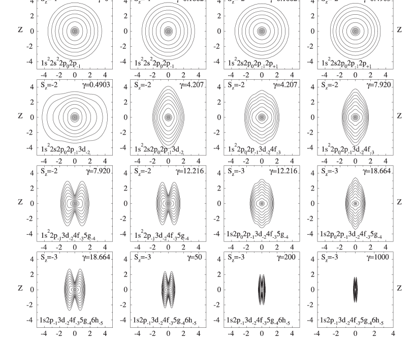
Figure 3: Contour plots of the total electronic densities for the ground state of the carbon atom. For neighbouring lines the densities are different by a factor of $e$. The coordinates $z$, $\rho$ as well as the corresponding field strengths are given in atomic units.

Figure 3 allows us to add some more informations to the considerations of the previous section. This figure presents spatial distributions of the total electronic densities for the ground state configurations of the carbon atom. More precisely, it allows us to gain insights into the geometry of the distribution of the electron density in space and in particular its dependence on the magnetic quantum number and the total spin. Thereby we can understand the corresponding impact on the total energy of the atom. The first picture in this figure presents the distribution of the electron density of the ground state of the carbon atom at $\gamma=0$. The following pictures show the distributions of the electronic densities at values of the field strength which mark the boundaries of the regimes of field strengths belonging to the different ground state configurations. For the high-field ground state we present the distribution of the electronic density at the crossover field strength $\gamma=18.664$ and for three additional values of $\gamma$ up to $\gamma=1000$.

For each configuration the effect of the increasing field strength consists in compressing the electronic distribution towards the $z$ axis. However most of the crossovers of ground state configurations involve the opposite effect which is due to the fact that they are associated with an increase of the total magnetic quantum number $M={\sum_{\mu=1}^{6}m_{\mu}}$.

For the lithium atom the analogous arguments and calculations IvaSchm98 lead to the scheme presented in table 2.

Table 2: The Hartree-Fock ground state configurations of the lithium atom in external magnetic fields. The configurations, presented in the table are the ground state configurations at $\gamma_{\rm min}\leq\gamma\leq\gamma_{\rm max}$.

no.	$\gamma_{\rm min}$	$\gamma_{\rm max}$	The ground state configuration	$M$	$S_{z}$	$E(\gamma_{\rm min})$
1	0	0.17633	$1s^{2}2s$	$0$	$-1/2$	$-7.43275$
2	0.17633	2.1530	$1s^{2}2p_{-1}$	$-1$	$-1/2$	$-7.48162$
3	2.1530	$\infty$	$1s2p_{-1}3d_{-2}$	$-3$	$-3/2$	$-7.64785$

V Ground state electronic configurations in the high-field regime

Let us consider now the series of neutral atoms and positive ions with $Z\leq 10$ in the high field domain which we define here as the one, where the ground state electronic configurations are fully spin polarised (Fully Spin Polarised (FSP) regime $S_{z}=-N/2$). The FSP regime supplies an additional advantage for calculations performed in the Hartree-Fock approach, because our one-determinant wave functions are eigenfunctions of the total spin operator ${\bf S^{2}}$. Starting from the high-field limit we investigate the electronic structure and properties of the ground states with decreasing field strength until we reach the first crossover to a partially spin polarised (PSP) configuration with $S_{z}=-N/2+1$.

The approach to this investigation is very similar to that described in the previous section and the picture of the crossovers associated with the ground states of atoms and positive ions $A^{+}$ is presented in table 3. It should be noted that, for atoms with $Z\leq 6$ and ions with $Z\leq 7$, the state $\left|1s^{2}\right>$ becomes the ground state while lowering the spin polarisation from the maximal absolute value $S_{z}=-N/2$ to $S_{z}=-N/2+1$. For heavier atoms and ions we remark that the state $\left|1s^{2}\right>$ is not the energetically lowest one in the PSP subset at magnetic field strengths for which its energy becomes equal to the energy of the lowest FSP state. For these atoms and ions the state $\left|1s^{2}2p_{0}\right>$ is energetically lower than $\left|1s^{2}\right>$ at these field strengths. For atoms with $Z\geq 7$ and positive ions with $Z\geq 8$ the intersection points between the state $\left|1s^{2}2p_{0}\right>$ and the energetically lowest state in the FSP subspace have to be calculated. In result, the spin-flip crossover occurs at higher fields than this would be in the case of $\left|1s^{2}\right>$ being the lowest state in the PSP subspace. In particular, the spin-flip crossover for the neon atom is found to be slightly higher than the point of the crossover $\left|2p_{0}\right>-\left|2p_{0}3d_{-1}\right>$, and, therefore, this atom has in the framework of the Hartree-Fock approximation only two fully spin polarised configurations likewise other neutral atoms and positive ions with $6\leq Z\leq 10$. It should be noted that the situation with the neon atom can be regarded as a transient one due to closeness of the intersection $\left|2p_{0}\right>-\left|2p_{0}3d_{-1}\right>$ to the intersection $\left|2p_{0}\right>-\left|1s^{2}2p_{0}\right>$. This means that we can expect the configuration $\left|2p_{0}3d_{-1}\right>$ to be the global ground state for the sodium atom ($Z=11$). In addition an investigation of the neon atom carried out on a more precise level than the Hartree-Fock method could also introduce some corrections to the picture described above for this atom.

Table 3: Total energies (a.u.) of the neutral atoms and ions ${\rm A^{+}}$ at the crossover points of the ground state configurations.

$Z$	$\gamma$	Atomic state(s)	$-E{\rm(Atomic)}$	Ionic state(s)	$-E{\rm(A^{+})}$
2	0.711	$\left|0_{N}\right>$, $\left|1s^{2}\right>$	2.76940	$\left|0_{N}\right>$	2.32488
3	2.153	$\left|0_{N}\right>$, $\left|1s^{2}\right>$	7.64785	$\left|0_{N}\right>$	7.00057
	2.0718	$\left|1s^{2}\right>$	7.65600	$\left|0_{N}\right>$, $\left|1s^{2}\right>$	6.94440
4	4.567	$\left|0_{N}\right>$, $\left|1s^{2}\right>$	15.9166	$\left|0_{N}\right>$	15.07309
	4.501	$\left|1s^{2}\right>$	15.91625	$\left|0_{N}\right>$, $\left|1s^{2}\right>$	15.01775
5	8.0251	$\left|0_{N}\right>$, $\left|1s^{2}\right>$	28.18667	$\left|0_{N}\right>$	27.16436
	7.957	$\left|1s^{2}\right>$	28.17996	$\left|0_{N}\right>$, $\left|1s^{2}\right>$	27.10004
6	18.664	$\left|0_{N}\right>$, $\left|2p_{0}\right>$	50.9257	$\left|0_{N}\right>$	49.50893
	14.536	$\left|2p_{0}\right>$	47.23836	$\left|0_{N}\right>$, $\left|2p_{0}\right>$	45.77150
	12.351	$\left|2p_{0}\right>$	45.07386	$\left|2p_{0}\right>$, $\left|1s^{2}\right>$	43.72095
	12.216	$\left|2p_{0}\right>$, $\left|1s^{2}\right>$	44.9341	$\left|1s^{2}\right>$	43.70075
7	36.849	$\left|0_{N}\right>$, $\left|2p_{0}\right>$	84.4186	$\left|0_{N}\right>$	82.58182
	30.509	$\left|2p_{0}\right>$	79.34493	$\left|0_{N}\right>$, $\left|2p_{0}\right>$	77.41246
	17.429	$\left|2p_{0}\right>$	66.72786	$\left|2p_{0}\right>$, $\left|1s^{2}\right>$	65.26170
	17.398	$\left|2p_{0}\right>$, $\left|1s^{2}2p_{0}\right>$	66.69306	$\left|1s^{2}\right>$	65.25362
8	64.720	$\left|0_{N}\right>$, $\left|2p_{0}\right>$	130.6806	$\left|0_{N}\right>$	128.4054
	55.747	$\left|2p_{0}\right>$	124.1125	$\left|0_{N}\right>$, $\left|2p_{0}\right>$	121.69825
	23.985	$\left|2p_{0}\right>$, $\left|1s^{2}2p_{0}\right>$	94.3773	$\left|2p_{0}\right>$	92.78308
	23.849	$\left|1s^{2}2p_{0}\right>$	94.3336	$\left|2p_{0}\right>$, $\left|1s^{2}2p_{0}\right>$	92.62502
9	104.650	$\left|0_{N}\right>$, $\left|2p_{0}\right>$	191.8770	$\left|0_{N}\right>$	189.1446
	92.624	$\left|2p_{0}\right>$	183.6944	$\left|0_{N}\right>$, $\left|2p_{0}\right>$	180.7819
	31.735	$\left|2p_{0}\right>$, $\left|1s^{2}2p_{0}\right>$	128.1605	$\left|2p_{0}\right>$	126.4414
	31.612	$\left|1s^{2}2p_{0}\right>$	128.1125	$\left|2p_{0}\right>$, $\left|1s^{2}2p_{0}\right>$	126.2897
10	159.138	$\left|0_{N}\right>$, $\left|2p_{0}\right>$	270.220	$\left|0_{N}\right>$	267.0112
	143.604	$\left|2p_{0}\right>$	260.2740	$\left|0_{N}\right>$, $\left|2p_{0}\right>$	256.8459
	40.672	$\left|2p_{0}\right>$, $\left|1s^{2}2p_{0}\right>$	168.4734	$\left|2p_{0}\right>$	166.6327
	40.559	$\left|1s^{2}2p_{0}\right>$	168.4217	$\left|2p_{0}\right>$, $\left|1s^{2}2p_{0}\right>$	166.4863

Summarising our results we remark that the atoms and positive ions with $Z\leq 5$ have one FSP ground state configuration $\left|0_{N}\right>$ whereas the atoms and ions with $6\leq Z\leq 10$ possess two such configurations $\left|0_{N}\right>$ and $\left|2p_{0}\right>$.

Figure 4: Relative errors of the total energy in the adiabatic approximation depending on the charge of the nucleus. $E_{\rm 1D}$ – the total energies in the adiabatic approximation ($B_{12}=0.1,\ 0.5,\ 1,\ 5$ [VII], $B_{12}=2.35$ [VII]), $E_{\rm 2D}$ – our two-dimensional mesh results. $B_{12}=B/10^{12}$G.

Possessing total energies for all the atoms with $Z\leq 10$ we can compare these results with the adiabatic calculations Neuhauser ; Godefroid . Both our results ($E_{\rm 2D}$) and calculations Neuhauser ; Godefroid ($E_{\rm 1D}$) are carried out in the adiabatic approximation. The difference between $E_{\rm 1D}$ and $E_{\rm 2D}$ consists only in the usage of the adiabatic approximation for obtaining energies $E_{\rm 1D}$ instead of exact solution of the Hartree-Fock equations for $E_{\rm 2D}$. Thus, the comparison of $E_{\rm 1D}$ and $E_{\rm 2D}$ allows us to evaluate the precision of the adiabatic approximation itself and obtain an idea of the degree of its applicability for multi-electron atoms for different field strengths and nuclear charges. All our values lie lower than the values of these adiabatic calculations. It is well known, that the precision of the adiabatic approximation decreases with decreasing field strength. The increase of the relative errors with decreasing field strength is clearly visible in the table. On the other hand, the relative errors of the adiabatic approximation possess the tendency to increase with growing $Z$, which is manifested by the scaling transformation $E(Z,\gamma)=Z^{2}E(1,\gamma/Z^{2})$ (e.g. Rud94 ; Ivanov94 ) well known for hydrogen-like ions. The behaviour of the inner electrons is to some extent similar to the behaviour of the electrons in the corresponding hydrogen-like ions. Therefore their behaviour is to lowest order similar to the behaviour of the electron in the hydrogen atom at magnetic field strength $\gamma/Z^{2}$ i.e. this behaviour can be less accurately described by the adiabatic approximation at large $Z$ values. The absolute values of the errors in the total energy associated with the adiabatic approximation are in many cases larger than the corresponding values of the ionisation energies.

VI Mesh approach for single-electron atomic and molecular systems in strong electric fields

In this section we present some features of our approach With respect to its application to systems in strong external electric fields and correspondingly some relevant physical results. In contrast to the situation discussed in the previous sections atoms and molecules in external uniform electric fields have no stationary states, because for every state there is a probability that one or several electrons leave the system. Thus, when switching on the external uniform electric field, all the stationary states turn into resonances. Using the complex form of the energy eigenvalues

$$E=E_{0}-i\Gamma/2$$

one may consider quasi-stationary states of quantum systems similarly to the stationary ones. In this approach the real part of the energy $E_{0}$ is the centre of the band corresponding to the quasi-stationary state and the imaginary part $\Gamma/2$ is the half-width of the band which determines the lifetime of the state. In this communication we consider systems which can be described by two-dimensional one-electron Hamiltonians. These systems include the hydrogen atom and the ${\rm H_{2}^{+}}$ molecular ion in an electric field Ivanov94a ; Ivanov98a ; Ivanov2001 and the hydrogen atom in parallel electric and magnetic fields Ivanov2001 ; Ivanov83VLGU . The only electron present in such a system can leave it under impact of the external electric field. From the mathematical point of view the problem consists in obtaining solutions of the single-particle Schrödinger equation for this electron with the correct asymptotic behaviour of the wavefunction as an outgoing wave. Currently we have three different possibilities for fixing this asymptotics realised in our computational program:

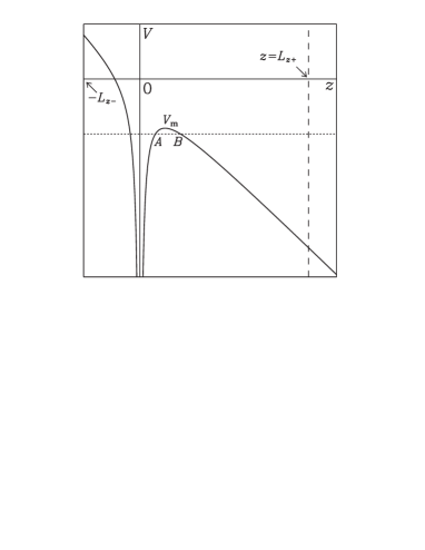
Figure 5: The potential energy for the hydrogen atom $V(\rho=0,z)$ in the external uniform electric field.

1. Complex boundary condition method. This method is described in detail in ref. Ivanov98a . The method is based on the fact that the single-electron Schrödinger equation for a finite system can be solved with the arbitrary precision in a finite area both for stationary and for quasi-stationary eigenstates. The case of stationary states is considered in ZhVychMat ; Ivanov88 . The approach for the quasi-stationary states will be discussed following Ivanov98a . Figure 5 presents the potential curve for the simplest Hamiltonian of the hydrogen atom in an electric field

$$H=-\frac{1}{2}\left(\frac{\partial^{2}}{\partial\rho^{2}}+\frac{1}{\rho}\frac{\partial}{\partial\rho}+\frac{\partial^{2}}{\partial z^{2}}-\frac{m^{2}}{\rho^{2}}\right)-\frac{1}{r}-Fz$$ (5)

$F$ is the electric field strength multiplied by the charge of the electron. Analogously to Ivanov83VLGU ; Ivanov88 the calculations can be carried out in an area $\Omega$ which is finite along the direction $z$. For this coordinate we used uniform meshes. The boundary of the area $z=-L_{z-}$ for $z<0$ ($F\geq 0$) (Figure 5) is determined from the condition of small values of the wavefunction on the boundary and, therefore, small perturbations introduced by the corresponding boundary condition Ivanov88 . The values of the wavefunction on the opposite boundary of the area ($z=L_{z+}$) cannot be excluded from the consideration. We consider non-stationary states of the system decaying into continuum of free particles. In this process an electron leaves the system in direction $z\rightarrow+\infty$ and, thus, an outgoing wave boundary condition is to be established on $z=L_{z+}$. The form of this boundary condition can be derived from the asymptotic behaviour of the wavefunction for $z\rightarrow+\infty$ and has the form

$$\left.\frac{\partial\psi}{\partial z}+\left(\frac{F}{2k^{2}}-ik\right)\psi\right|_{z=L_{z+}}=0$$ (6)

where $k=[2(E+Fz)]^{1/2}$ is the wavenumber. Solving the Schrödinger equation with the Hamiltonian (5) and the boundary condition (6) established on a reasonable distance $L_{z+}$ from the origin of the system we can obtain the complex eigenvalues of the energy and the wavefunctions of the type presented in the Figure 6.

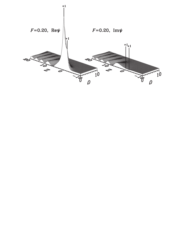
Figure 6: Real and imaginary parts of the wavefunction of the $\rm H_{2}^{+}$ molecule in a longitudinal electric field $F$ (a.u.).

This straightforward approach enables obtaining precise results both for atoms and molecules from weak to moderate strong fields (for instance for the ground state of the hydrogen atom up to $F=0.20-0.25$ a.u.).

2. Classical complex rotation of the coordinate $z$ in the form $z\rightarrow ze^{i\Theta}$. In this approach we have obtained precise results for atomic systems in strong fields from the lower bound of the over-barrier regime up to superstrong fields corresponding to regime $|{\rm Re}E|<<|{\rm Im}E|$ Ivanov2001 . On the other hand, this method cannot be immediately applied to molecular systems in our direct mesh approach Simon79 ; Ivanov2001 .

3. Exterior complex transformation of the coordinate $z$. In our numerical approach we transform the real coordinate $z$ into a curved path in the complex plane $z$. This transformation leaves intact the Hamiltonian in the internal part of the system, but supplies the complex rotation of $z$ (and the possibility to use the zero asymptotic boundary conditions for the wavefunction) in the external part of the system. The transformation can be applied both for atoms and molecules and provides precise results for fields from weak up to superstrong with some decrease of the numerical precision in the regime $|{\rm Re}E|<<|{\rm Im}E|$ Ivanov2001 .

The numerical results obtained by all three methods coincide And are in agreement with numerous published data on the hydrogen atom in electric fields (see e.g. Kolosov87 ; Kolosov89 ; NicolaG ; NicolaT and references in Ivanov98a ).

Some of our results for the hydrogen atom in parallel electric and magnetic fields Ivanov2001 are shown in Table 4.

Table 4: The ground state of the hydrogen atom in parallel electric and magnetic fields at $F=0.1,\ 1,\ 5$.

	$F=0.1$		$F=1$		$F=5$
$\gamma$	$E_{0}$	$\Gamma/2$	$E_{0}$	$\Gamma/2$	$E_{0}$	$\Gamma/2$
$0$	$-0.5274183$	$7.26904(-3)$	$-0.6243366$	$0.6468208$	$-0.1350071$	$3.083929$
$0.01$	$-0.532390$	$7.2624(-3)$	$-0.629329$	$0.646812$	$-0.140005$	$3.083925$
$0.1$	$-0.574600$	$6.6392(-3)$	$-0.673584$	$0.646053$	$-0.184739$	$3.083589$
$1$	$-0.8443098$	$9.5923(-5)$	$-1.0421379$	$0.577291$	$-0.6077008$	$3.050207$
$10$	$-1.7498730$	—	$-1.9579187$	$0.1173924$	$-2.375552$	$1.955678$
$100$	$-3.790110$	—	$-3.8219215$	$4.9988(-5)$	$-4.3806709$	$0.4909467$
$1000$	$-7.66247$	—	$-7.66807$	—	$-7.82561$	$1.04701(-2)$

       

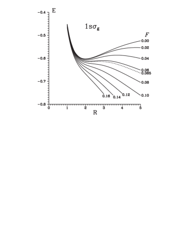
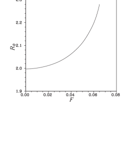
Figure 7: Left – Potential curves for the ground state of the $\rm H_{2}^{+}$ molecule in longitudinal electric field $F$ (a.u.). Right - The equilibrium internuclear distance of the molecule $\rm H_{2}^{+}$ as a function of the applied electric field strength.

Table 5: Equilibrium internuclear distances and corresponding energies and half-widths of the energy of the ground state of $\rm H_{2}^{+}$ molecule in longitudinal electric fields.

$F$	$R_{0}$	$E_{0}$	$\Gamma/2$	$F$	$R_{0}$	$E_{0}$	$\Gamma/2$
0.00	1.997	-0.60264	—	0.04	2.062	-0.60686	1.23(-19)
0.01	2.001	-0.60289	—	0.05	2.112	-0.60943	7.32(-15)
0.02	2.012	-0.60366	—	0.06	2.198	-0.61285	1.49(-11)
0.03	2.031	-0.60497	—	0.065	2.28	-0.61501	3.94(-10)

The second system which we present in this section is the hydrogen molecular ion $\rm H_{2}^{+}$ in a strong longitudinal electric field. Our approach allowed us to carry out the first correct consideration of this system Ivanov94a and, in particular, to obtain the potential curves of its ground state, presented in Figure 7 (left). The minima in these curves give the equilibrium internuclear distances, presented in this Figure (right) as a function of the electric field strength. One can see that at a critical value of the electric field about 0.065 a.u. the minimum disappears and, thus, above this critical value the hydrogen molecular ion cannot exist. This critical value of the maximal electric field $F_{\rm c}=0.065{\rm a.u.}=3.3{\rm V/\AA}$ for the molecule $\rm H_{2}^{+}$ is in a good agreement with experimental results by Bucksbaum90 . According this work $\rm H_{2}^{+}$ molecule may exist in laser beam fields with intensity less than $10^{14}{\rm W/cm^{2}}$ which corresponds to $3{\rm V/\AA}$, and does not exist in more intense fields.

VII Conclusions

In this communication we have presented a 2D fully numerical mesh solution method in its various applications to atoms and simple diatomic molecules in strong external electric and magnetic fields. Specifically these are calculations of atoms with $Z\leq 10$ and their positive ions in strong magnetic fields and the comprehensive investigation of the electronic structure of the ground states of the Li and C atoms in arbitrary magnetic fields. For the carbon atom seven different electronic ground state configurations for different domains of the magnetic field strength have been found. The investigation of the series of atoms with $Z\leq 10$ in very strong magnetic fields enables us to evaluate the applicability of the adiabatic approximation and to show its decreasing precision for heavier atoms.

The mathematical technique developed for solving Schrödinger equations for quasi-steady states allowed us to obtain a series of results for the hydrogen atom in parallel electric and magnetic fields and for the ${\rm H_{2}^{+}}$ ion in strong electric fields.

Thus, the method described above allows us to obtain a number of new physical results partially presented in this communication. These calculations are carried out in the Hartree-Fock approximation for multi-electron systems and are exact solutions of the Schrödinger equation for the single-electron case. As the following development of the method we plan to implement the configuration interaction approach in order to study correlation effects in multi-electron systems both in electric and magnetic fields.

References

- (1) Friedrich, H.; Wintgen, D. Phys.Rep. 1989, 183, 37.
- (2) Rösner, W.; Wunner, G.; Herold, H.; Ruder, H. J. Phys. B: At. Mol. Opt. Phys. 1984, 17, 29.
- (3) Ivanov, M.V. J. Phys. B: At. Mol. Opt. Phys. 1988, 21, 447.
- (4) Kravchenko, Yu.P.; Liberman, M.A.; Johansson, B. Phys.Rev.Lett. 1996, 77, 619.
- (5) Elliott, R.J.; Loudon, R. J. Phys. Chem. Sol. 1960, 15 196.
- (6) Neuhauser, D.; Koonin, S.E.; Langanke, K. Phys. Rev. A 1986, 33, 2084; 1987, 36, 4163.
- (7) Demeur, M.; Heenen, P.-H.; Godefroid, M. Phys. Rev. A 1994, 49, 176.
- (8) Garstang, R.H. Rep. Prog. Phys. 1977, 40, 105.
- (9) Simola, J.; Virtamo, J. J. Phys. B 1978, 11, 3309.
- (10) Friedrich, H. Phys. Rev. A 1982, 26, 1827.
- (11) Fonte, G.; Falsaperla, P.; Schriffer, G.; Stanzial, D. Phys. Rev. A 1990, 41, 5807.
- (12) Schmidt, H.M. J. Phys. B: At. Mol. Opt. Phys. 1991, 24, 2947.
- (13) Mueller, R.O.; Rao, A.R.P.; Spruch, L. Phys. Rev. A 1975, 11, 789.
- (14) Virtamo, J. J. Phys. B: At. Mol. Phys. 1976, 9, 751.
- (15) Larsen, D.M. Phys. Rev. B. 1979, 20, 5217.
- (16) Gadiyak, G.V.; Lozovik, Yu.E.; Mashchenko, A.I.; Obrecht, M.S. J. Phys. B: At. Mol. Phys. 1982, 15, 2615.
- (17) Vincke, M.; Baye, D. J. Phys. B: At. Mol. Opt. Phys. 1989, 22, 2089.
- (18) Ivanov, M.V. Opt. Spektrosk. 1991, 70, 259; English transl.: Opt. Spectrosc. 1991, 70, 148.
- (19) Thurner, G.; Körbel, H.; Braun, M.; Herold, H.; Ruder, H.; Wunner G. J. Phys. B: At. Mol. Opt. Phys. 1993, 26, 4719.
- (20) Ivanov, M.V. J. Phys. B: At. Mol. Opt. Phys. 1994, 27, 4513.
- (21) Jones, M.D.; Ortiz, G.; Ceperley, D.M. Phys. Rev. A. 1996, 54, 219.
- (22) Jones, M.D.; Ortiz, G.; Ceperley, D.M. Phys. Rev. E 1997, 55, 6202; Phys. Rev. A 1999, 59, 2875.
- (23) Henry, R.J.; O’Connell, R.F.; Smith, E.R.; Chanmugam, G.; Rajagopal, A.K. Phys. Rev. D 1974, 9, 329.
- (24) Surmelian, G.L.; Henry, R.J.; O’Connell, R.F. Phys. Lett. A 1974, 49, 431.
- (25) Becken, W.; Schmelcher, P.; Diakonos, F.K. J. Phys. B: At. Mol. Opt. Phys. 1999, 32, 1557.
- (26) Becken, W.; Schmelcher, P. J. Phys. B: At. Mol. Opt. Phys. 2000, 33, 545.
- (27) Müller, E. Astron. & Astrophys. 1984, 130, 415.
- (28) Ivanov, M.V. Phys. Lett. A 1998, 239, 72.
- (29) Ivanov, M.V.; Schmelcher, P. Phys. Rev. A 1998, 57, 3793.
- (30) Ivanov, M.V.; Schmelcher, P. Phys. Rev. A 1999, 60, 3558.
- (31) Ivanov, M.V.; Schmelcher, P. Phys. Rev. A 2000, 61, 022505.
- (32) Laaksonen, L.; Pyykkö, P.; Sundholm, D. Chem. Phys. Lett. 1983, 96, 1.
- (33) Kobus, J. Chem. Phys. Lett. 1993, 202, 7.
- (34) Vincke, M.; Malegat, L.; Baye, D. J. Phys. B: At. Mol. Opt. Phys. 1993, 26, 811.
- (35) Abramowitz, M.; Stegun, I.A.; eds. “Handbook of Mathematical Functions”; Dover Publications: New York, 1972, 787.
- (36) Ruder, H.; Wunner, G.; Herold, H.; Geyer, F. “Atoms in Strong Magnetic Fields”; Springer-Verlag, 1994.
- (37) Ivanov, M.V. Opt. Spektrosk. 1994, 76, 711. English transl.: Opt. Spectrosc. 1994, 76, 631.
- (38) Ivanov, M.V. J. Phys. B: At. Mol. Opt. Phys. 1998, 31, 2833.
- (39) Ivanov, M.V. to be published.
- (40) Anokhin, S.B.; Ivanov, M.V. Vestn. Leningr. Univ. Fiz. & Khim. 1983, no.2, 65.
- (41) Ivanov, M.V. USSR Comput. Math. & Math. Phys. 1986, 26, 140.
- (42) Simon, B. Phys. Lett. A 1979, 71, 211.
- (43) Kolosov, V.V. J. Phys. B: At. Mol. Phys. 1987, 20, 2359.
- (44) Kolosov, V.V. J. Phys. B: At. Mol. Opt. Phys. 1989, 22, 833.
- (45) Nicolaides, C.A.; Gotsis, H.J. J. Phys. B: At. Mol. Opt. Phys. 1992, 25, L171.
- (46) Nicolaides, C.A.; Themelis, S.I. Phys. Rev. A 1992, 45, 349.
- (47) Bucksbaum, P.H.; Zavriyev, A.; Muller, H.G.; Schumacher, D.W. Phys. Rev. Lett. 1990, 1883.