A new approach to study energy transfer in magnetohydrodynamic turbulence

Abstract

The unit of nonlinear interaction in Navier-Stokes and the Magnetohydrodynamic (MHD) equations is a wavenumber triad (k,p,q) satisfying ${\bf k+p+q=0}$. The expression for the combined energy transfer from two of these wavenumbers to the third wavenumber is known. In this paper we introduce the idea of an effective energy transfer between a pair of modes through the mediation of the third mode and then find an expression for it. In fluid turbulence, energy transfer takes place between a pair of velocity modes, whereas in MHD turbulence energy transfer takes places between (1) a pair of velocity modes, (2) a pair of magnetic modes, and (3) between a velocity and a magnetic mode in a triad. In this paper we have obtained the expression for each of these transfers. We also show how the effective mode-to-mode energy transfer rate can be utilised to study energy cascades and shell-to-shell energy transfer rates.

I Introduction

In fluid and MHD turbulence, eddies of various sizes interact amongst themselves; energy is exchanged among them in this process. These interactions arise due to the nonlinearity present in these systems. The fundamental interactions involve wavenumber triads (k,p,q) with ${\bf k+p+q=0}$.

The combined energy transfer computation to a mode from the other two modes of a triad has generally been considered to be fundamental. This formalism has played an important role in furthering our understanding of locality in fluid turbulence  [1, 2, 3, 4], and also in analysing subgrid scale eddy viscosity  [5, 6]. Energy interactions are considered to be local if the triads with $k\sim p\sim q$ contribute most to the energy transfer to the wavenumber $k$. Numerical simulations of Domaradzki and Rogallo  [2, 1] showed that the contribution of the nonlocal triads ($k\sim p>>q$) to the interactions is not small, but in such triads the dominant exchange of energy occurs between wavenumbers of similar magnitudes, i.e., between $k$ and $p$. Domaradzki et al.  [6] computed the sub-grid scale viscosity by summing up the energy lost by a wavenumber $k<k_{c}$ (cut off wavenumber) by triad interactions with atleast one wavenumber larger than $k_{c}$. Batchelor  [7] first suggested a formula for the energy transfer in fluid turbulence between two regions in Fourier space, and Domaradzki and Rogallo  [1] calculated shell-to-shell energy transfer rates. Taking energy transfer between shells as an example, we will show in Section III, that these formalisms have certain limitations.

In this paper we present a scheme to calculate the energy transfer rates between two modes in a triad interaction. Using our scheme we can calculate the energy transfer rates between two shells, cascade rates, and also study locality of energy transfer. The formulae for the combined energy transfer rate were used to study energy transfer rates in MHD turbulence  [8, 9, 10, 11, 12]. Ishizawa and Hattori  [12] numerically computed the kinetic energy flux to the velocity modes outside the sphere and the magnetic energy fluxes to the magnetic modes outside the sphere. They also computed the kinetic energy fluxes due to transfer of energy to all magnetic modes and a similar magnetic energy flux due to transfer of energy to all velocity modes  [12]. Pouquet et al.  [9], Pouquet  [10], and Ishizawa and Hattori  [11] used the combined energy transfer formalism in an Eddy damped quasi-normal Markovian (EDQNM) closure calculation to study non-local energy transfer. However, several energy transfers cannot be calculated using these formalisms. Our formalism of “mode-to-mode” transfer enables us to calculate all these energy transfer rates between the spheres and the shells.

This paper is organized into the following sections. In Section II we will state the known results regarding the combined energy transfer between velocity modes of a triad. In Section III we will present a discussion on the formulae which are used for studying energy transfer between shells in fluid turbulence. In Section IV we will formulate a way of studying energy transfer between a pair of modes within a triad, with the third mode of the triad meditating the transfer. This new method is used to re-define shell-to-shell transfer in Section V. The known results of energy transfer in a MHD triad are discussed in Section VI and the “mode-to-mode” transfers in MHD in Section VII. The results of Section VII are used in Section VIII to define shell-to-shell transfer rates and the energy cascade rates in MHD turbulence. The conclusions of this paper follows in Section IX.

II Energy transfer in a triad: Known results

The Navier Stokes equation in real space are written as

$$\frac{\partial{\bf u}}{\partial t}+({\bf u.\nabla}){\bf u}=-{\bf\nabla}p+\nu{\bf\nabla^{2}u},$$ (1)

where ${\bf u}$ is the velocity field, and $\nu$ is the fluid kinematic viscosity. In Fourier space, the kinetic energy equations for a Fourier mode is

$$\frac{\partial E^{u}(\bf k)}{\partial t}+2\nu k^{2}E^{u}({\bf k})=\sum_{{\bf k+p+q}=0}\frac{1}{2}S^{uu}({\bf k|p,q}),$$ (2)

where $E^{u}({\bf k})\equiv{\bf|u(k)|}^{2}/2$ is the kinetic energy in Fourier space for mode k. The nonlinear term $S^{uu}({\bf k|p,q})$ is

$$S^{uu}({\bf k|p,q})\equiv-Re\left(i{\bf\left[k.u(q)\right]}{\bf\left[u(k).u(p)\right]}+i{\bf\left[k.u(p)\right]}{\bf\left[u(k).u(q)\right]}\right)$$ (3)

This term represents the combined transfer of kinetic energy from mode ${\bf p}$ and ${\bf q}$ to mode ${\bf k}$  [13]. Note that the wavenumber triad $\bf k$, $\bf p$, and $\bf q$ should satisfy the condition ${\bf k+p+q}=0$. This nonlinear term satisfies the following conservation property

$$S^{uu}({\bf k|p,q})+S^{uu}({\bf p|k,q})+S^{uu}({\bf q|k,p})=0.$$ (4)

While the quantity $S^{uu}({\bf k|p,q})$ represents the nonlinear energy transfer from the two modes $\bf p$ and $\bf q$ to mode $\bf k$, it would be useful to know the exact energy transfer between any two modes, say from ${\bf p}$ to ${\bf k}$. In Section IV we will explore this idea.

III Shell-to-Shell energy transfer in fluid turbulence

Using the combined energy transfer $S^{uu}({\bf k|p,q})$, Domaradzki and Rogallo  [1] have discussed energy transfer between two shells. They interpret the quantity

$$T^{uu}_{mn}=\frac{1}{2}\sum_{{\bf k}{\epsilon}{\it m}}\sum_{{\bf p}{\epsilon{\it n}}}S^{uu}({\bf k|p,q}).$$ (5)

as the rate of energy transfer from shell n to shell m  [1, 7]. Note that k-sum is over shell m, p-sum over shell n, and ${\bf q=-k-p}$. However, Domaradzki and Rogallo  [1] themselves points out that it may not be entirely correct to interpret the formula (5) as the shell-to-shell energy transfer. The reason for this is as follows:

In the energy transfer between two shells m and n, two types of wavenumber triads are involved (see Fig. 1 shown below). In a triad of type I, the wavenumbers p, q are located in one shell, and k is located in the other. In a type II triad, wavenumber k is in one shell, p or q in the other shell, and the third wavenumber is located outside the two shells. In Eq. (5) the summation is carried over both kinds of triads. However, it is easy to see that the energy transfer from shell n to shell m takes place through both the k-p and k-q legs of triad I but only through the k-p leg of triad II. Hence Batchelor’s and Domaradzki’s formalism do not yield correct shell-to-shell energy transfers (as was pointed out by Batchelor and Domaradzki themselves).

IV Mode-to-Mode energy transfer in a triad

The nonlinear interaction in the Navier-Stokes and the MHD equations are intrinsically three-mode interactions. The expression for the energy transfer to one mode of the triad from the other two was presented in Section II. In this section we shall explore the possibility of obtaining an expression for the energy transfer between any two modes within a triad — we will call it the mode-to-mode transfer. We emphasize that this approach is still within the framework of the triad interaction — that is, the triad is still the fundamental interaction of which the mode-to-mode transfer is a part. The energy transfer between two modes of a triad by the mediation of the third mode is sought here.

We shall first consider only the Navier-Stokes equation. In a later section, the discussion will be generalised to the MHD equation.

A Definition of Mode-to-Mode transfer in a triad

Consider a triad k, p, q. Let the quantity ${\cal{R\hskip-7.67015pt\hbox to7.67015pt{\hss\sl/\/\hss}}}^{uu}({\bf k|p|q})$ denote the energy transferred from mode p to mode k with mode q playing the role of a mediator (see Fig. 2). We wish to obtain an expression for ${\cal{R\hskip-7.67015pt\hbox to7.67015pt{\hss\sl/\/\hss}}}^{uu}$.

The ${\cal{R\hskip-7.67015pt\hbox to7.67015pt{\hss\sl/\/\hss}}}^{uu}$’s should satisfy the following relationships :

1. The sum of ${\cal{R\hskip-7.67015pt\hbox to7.67015pt{\hss\sl/\/\hss}}}^{uu}({\bf k|p|q})$ and ${\cal{R\hskip-7.67015pt\hbox to7.67015pt{\hss\sl/\/\hss}}}^{uu}({\bf k|q|p})$, which represent energy transfer from mode p to mode k and from mode q to mode k, respectively, should be equal to the total energy transferred to mode k from modes p and q, i.e., $S^{uu}({\bf k|p,q})$ [see Eq. (3)]. Thus,

   $${\cal{R\hskip-7.67015pt\hbox to7.67015pt{\hss\sl/\/\hss}}}^{uu}({\bf k|p|q})+{\cal{R\hskip-7.67015pt\hbox to7.67015pt{\hss\sl/\/\hss}}}^{uu}({\bf k|q|p})=S^{uu}({\bf k|p,q}),$$ (6)

   $${\cal{R\hskip-7.67015pt\hbox to7.67015pt{\hss\sl/\/\hss}}}^{uu}({\bf p|k|q})+{\cal{R\hskip-7.67015pt\hbox to7.67015pt{\hss\sl/\/\hss}}}^{uu}({\bf p|q|k})=S^{uu}({\bf p|k,q}),$$ (7)

   $${\cal{R\hskip-7.67015pt\hbox to7.67015pt{\hss\sl/\/\hss}}}^{uu}({\bf q|k|p})+{\cal{R\hskip-7.67015pt\hbox to7.67015pt{\hss\sl/\/\hss}}}^{uu}({\bf q|p|k})=S^{uu}({\bf q|k,p}).$$ (8)

2. The energy transferred from mode p to mode k, i.e., ${\cal{R\hskip-7.67015pt\hbox to7.67015pt{\hss\sl/\/\hss}}}^{uu}({\bf k|p|q})$, will be equal and opposite to the energy transferred from mode k to mode p i.e., ${\cal{R\hskip-7.67015pt\hbox to7.67015pt{\hss\sl/\/\hss}}}^{uu}({\bf p|k|q})$. Thus,

   $${\cal{R\hskip-7.67015pt\hbox to7.67015pt{\hss\sl/\/\hss}}}^{uu}({\bf k|p|q})+{\cal{R\hskip-7.67015pt\hbox to7.67015pt{\hss\sl/\/\hss}}}^{uu}({\bf p|k|q})=0,$$ (9)

   $${\cal{R\hskip-7.67015pt\hbox to7.67015pt{\hss\sl/\/\hss}}}^{uu}({\bf k|q|p})+{\cal{R\hskip-7.67015pt\hbox to7.67015pt{\hss\sl/\/\hss}}}^{uu}({\bf q|k|p})=0,$$ (10)

   $${\cal{R\hskip-7.67015pt\hbox to7.67015pt{\hss\sl/\/\hss}}}^{uu}({\bf p|q|k})+{\cal{R\hskip-7.67015pt\hbox to7.67015pt{\hss\sl/\/\hss}}}^{uu}({\bf q|p|k})=0.$$ (11)

These are six equations with six unknowns. However, the value of the determinant formed from the Eqs. (6)-(11) is zero. Therefore we cannot find unique ${\cal{R\hskip-7.67015pt\hbox to7.67015pt{\hss\sl/\/\hss}}}^{uu}$’s given just these equations. However, it is reasonable to expect that there is a definite amount of energy transfer from one mode to the other mode, say from mode k to mode p given u(k), u(p), u(q). Since Eqs. (6)-(11) do not yield a unique ${\cal{R\hskip-7.67015pt\hbox to7.67015pt{\hss\sl/\/\hss}}}^{uu}$, we need to use constraints based on invariance, symmetries, etc. to get a definite ${\cal{R\hskip-7.67015pt\hbox to7.67015pt{\hss\sl/\/\hss}}}^{uu}$ using Eqs. (6)-(11).

B Solutions of equations of mode-to-mode transfer

One solution of Eqs. (6)-(11) is

$${\cal{S\hskip-6.70831pt\hbox to6.70831pt{\hss\sl/\/\hss}}}^{uu}({\bf k|p|q})\equiv-Re\left(i{\bf\left[k.u(q)\right]}{\bf\left[u(k).u(p)\right]}\right),$$ (12)

From the definition of ${\cal{S\hskip-6.70831pt\hbox to6.70831pt{\hss\sl/\/\hss}}}^{uu}({\bf k|p|q})$, it directly follows that ${\cal{S\hskip-6.70831pt\hbox to6.70831pt{\hss\sl/\/\hss}}}^{uu}$’s satisfy the following conditions.

$${\cal{S\hskip-6.70831pt\hbox to6.70831pt{\hss\sl/\/\hss}}}^{uu}({\bf k|p|q})+{\cal{S\hskip-6.70831pt\hbox to6.70831pt{\hss\sl/\/\hss}}}^{uu}({\bf k|q|p})=S^{uu}({\bf k|p,q}),$$ (13)

$${\cal{S\hskip-6.70831pt\hbox to6.70831pt{\hss\sl/\/\hss}}}^{uu}({\bf p|k|q})+{\cal{S\hskip-6.70831pt\hbox to6.70831pt{\hss\sl/\/\hss}}}^{uu}({\bf p|q|k})=S^{uu}({\bf p|k,q}),$$ (14)

$${\cal{S\hskip-6.70831pt\hbox to6.70831pt{\hss\sl/\/\hss}}}^{uu}({\bf q|k|p})+{\cal{S\hskip-6.70831pt\hbox to6.70831pt{\hss\sl/\/\hss}}}^{uu}({\bf q|p|k})=S^{uu}({\bf q|k,p}).$$ (15)

Using the triad relationship ${\bf k+p+q=0}$, and the incompressibility constraint [${\bf k.u(k)=0}$], it can be seen that ${\cal{S\hskip-6.70831pt\hbox to6.70831pt{\hss\sl/\/\hss}}}^{uu}$’s, etc. also satisfy the following conditions

$${\cal{S\hskip-6.70831pt\hbox to6.70831pt{\hss\sl/\/\hss}}}^{uu}({\bf k|p|q})+{\cal{S\hskip-6.70831pt\hbox to6.70831pt{\hss\sl/\/\hss}}}^{uu}({\bf p|k|q})=0,$$ (16)

$${\cal{S\hskip-6.70831pt\hbox to6.70831pt{\hss\sl/\/\hss}}}^{uu}({\bf k|q|p})+{\cal{S\hskip-6.70831pt\hbox to6.70831pt{\hss\sl/\/\hss}}}^{uu}({\bf q|k|p})=0,$$ (17)

$${\cal{S\hskip-6.70831pt\hbox to6.70831pt{\hss\sl/\/\hss}}}^{uu}({\bf p|q|k})+{\cal{S\hskip-6.70831pt\hbox to6.70831pt{\hss\sl/\/\hss}}}^{uu}({\bf q|p|k})=0.$$ (18)

Comparing Eqs. (13)-(18) with Eqs. (6)-(11), it is clear that the set of ${\cal{S\hskip-6.70831pt\hbox to6.70831pt{\hss\sl/\/\hss}}}^{uu}$’s is one instance of the ${\cal{R\hskip-7.67015pt\hbox to7.67015pt{\hss\sl/\/\hss}}}^{uu}$’s, i.e., ${\cal{R\hskip-7.67015pt\hbox to7.67015pt{\hss\sl/\/\hss}}}^{uu}({\bf k|p|q})={\cal{S\hskip-6.70831pt\hbox to6.70831pt{\hss\sl/\/\hss}}}^{uu}({\bf k|p|q})$. However, this is not a unique solution.

If another solution ${\cal{R\hskip-7.67015pt\hbox to7.67015pt{\hss\sl/\/\hss}}}^{uu}({\bf k|p|q})$ differs from ${\cal{S\hskip-6.70831pt\hbox to6.70831pt{\hss\sl/\/\hss}}}^{uu}({\bf k|p|q})$ by an arbitrary function $X_{\Delta}$, i.e., ${\cal{R\hskip-7.67015pt\hbox to7.67015pt{\hss\sl/\/\hss}}}^{uu}({\bf k|p|q})={\cal{S\hskip-6.70831pt\hbox to6.70831pt{\hss\sl/\/\hss}}}^{uu}({\bf k|p|q})+X_{\Delta}$, then by inspection we can easily see that every possible solution of Eqs. (6)-(11) must be of the form

$${\cal{R\hskip-7.67015pt\hbox to7.67015pt{\hss\sl/\/\hss}}}^{uu}({\bf k|p|q})={\cal{S\hskip-6.70831pt\hbox to6.70831pt{\hss\sl/\/\hss}}}^{uu}({\bf k|p|q})+X_{\Delta}$$ (19)

$${\cal{R\hskip-7.67015pt\hbox to7.67015pt{\hss\sl/\/\hss}}}^{uu}({\bf k|q|p})={\cal{S\hskip-6.70831pt\hbox to6.70831pt{\hss\sl/\/\hss}}}^{uu}({\bf k|q|p})-X_{\Delta}$$ (20)

$${\cal{R\hskip-7.67015pt\hbox to7.67015pt{\hss\sl/\/\hss}}}^{uu}({\bf p|k|q})={\cal{S\hskip-6.70831pt\hbox to6.70831pt{\hss\sl/\/\hss}}}^{uu}({\bf p|k|q})-X_{\Delta}$$ (21)

$${\cal{R\hskip-7.67015pt\hbox to7.67015pt{\hss\sl/\/\hss}}}^{uu}({\bf p|q|k})={\cal{S\hskip-6.70831pt\hbox to6.70831pt{\hss\sl/\/\hss}}}^{uu}({\bf p|q|k})+X_{\Delta}$$ (22)

$${\cal{R\hskip-7.67015pt\hbox to7.67015pt{\hss\sl/\/\hss}}}^{uu}({\bf q|k|p})={\cal{S\hskip-6.70831pt\hbox to6.70831pt{\hss\sl/\/\hss}}}^{uu}({\bf q|k|p})+X_{\Delta}$$ (23)

$${\cal{R\hskip-7.67015pt\hbox to7.67015pt{\hss\sl/\/\hss}}}^{uu}({\bf q|p|k})={\cal{S\hskip-6.70831pt\hbox to6.70831pt{\hss\sl/\/\hss}}}^{uu}({\bf q|p|k})-X_{\Delta}$$ (24)

Note that $X_{\Delta}$ can depend upon the wavenumber triad k, p, q, and the Fourier components u(k), u(p), u(q). $X_{\Delta}$ needs to be determined from other symmetry and invariance arguments to uniquely fix ${\cal{R\hskip-7.67015pt\hbox to7.67015pt{\hss\sl/\/\hss}}}^{uu}$.

In Appendix A we have attempted to determine $X_{\Delta}$. We construct $X_{\Delta}$ by observing that it can depend on k, p, q, u(k), u(p), u(q); and it must satisfy rotational invariance, galilean invariance, and it should be finite. In our procedure we write down a general scalar function of k, p, q, u(k), u(p), and u(q) with undetermined coefficients. The coefficients can be written as a series in the scalars of the type k.p, k.u(p), u(k).u(p) with unknown constants. By imposing invariance,and finiteness constraints we have shown that, upto the linear order in these scalars, the coefficients must vanish, giving $X_{\Delta}=0$. Unfortunately, we have not been able to determine the higher order coefficients. Hence, from the analysis of Appendix A we cannot show that $X_{\Delta}$ will definitely vanish. However, if $X_{\Delta}=0$ we get a simple relationship,

$${\cal{R\hskip-7.67015pt\hbox to7.67015pt{\hss\sl/\/\hss}}}^{uu}={\cal{S\hskip-6.70831pt\hbox to6.70831pt{\hss\sl/\/\hss}}}^{uu},$$ (25)

giving the energy transfer between a pair of modes in a triad with the third mode mediating the transfer, as simply ${\cal{S\hskip-6.70831pt\hbox to6.70831pt{\hss\sl/\/\hss}}}^{uu}$. But if $X_{\Delta}\neq 0$ then the energy transfer picture is more complex and the energy transfer between a pair of modes will be given by Eqs. (19)-(24) where $X_{\Delta}$ is unknown. However, even if $X_{\Delta}$ is unknown we can obtain very relevant information from the ${\cal{S\hskip-6.70831pt\hbox to6.70831pt{\hss\sl/\/\hss}}}^{uu}$’s as is shown below.

We will now give a physical interpretation to the two parts of ${\cal{R\hskip-7.67015pt\hbox to7.67015pt{\hss\sl/\/\hss}}}^{uu}$’s, i.e., ${\cal{S\hskip-6.70831pt\hbox to6.70831pt{\hss\sl/\/\hss}}}^{uu}$’s and $X_{\Delta}$. We now see from Fig. 3 that ${\cal{S\hskip-6.70831pt\hbox to6.70831pt{\hss\sl/\/\hss}}}^{uu}({\bf k|p|q})+X_{\Delta}$ gets transferred from p to k, ${\cal{S\hskip-6.70831pt\hbox to6.70831pt{\hss\sl/\/\hss}}}^{uu}({\bf q|k|p})+X_{\Delta}$ gets transferred from k to q, ${\cal{S\hskip-6.70831pt\hbox to6.70831pt{\hss\sl/\/\hss}}}^{uu}({\bf p|q|k})+X_{\Delta}$ gets transferred from q to p. The quantity $X_{\Delta}$ flows along ${\bf p}\rightarrow{\bf k}\rightarrow{\bf q}\rightarrow{\bf p}$, circulating around the entire triad without changing the energy of any of the modes. Therefore we will call it the Circulating transfer. Of the total energy transfer between two modes, ${\cal{S\hskip-6.70831pt\hbox to6.70831pt{\hss\sl/\/\hss}}}^{uu}+X_{\Delta}$, only ${\cal{S\hskip-6.70831pt\hbox to6.70831pt{\hss\sl/\/\hss}}}^{uu}$ can bring about a change in modal energy. $X_{\Delta}$ transferred from mode p to mode k is transferred back to mode p via mode q, i.e., the mode p transfers $X_{\Delta}$ directly to mode k, and mode p transfers $X_{\Delta}$ back to ${\bf k}$ indirectly through mode q. Thus the energy that is effectively transferred from mode p to mode k is just ${\cal{S\hskip-6.70831pt\hbox to6.70831pt{\hss\sl/\/\hss}}}^{uu}({\bf k|p|q})$. Therefore ${\cal{S\hskip-6.70831pt\hbox to6.70831pt{\hss\sl/\/\hss}}}^{uu}({\bf k|p|q})$ can be be termed as the effective mode-to-mode transfer from mode p to mode k.

In summary, we have attempted to obtain an expression for the energy transfer rate ${\cal{R\hskip-7.67015pt\hbox to7.67015pt{\hss\sl/\/\hss}}}^{uu}$ between two modes in a triad. To leading order in a series expansion, we can show that ${\cal{R\hskip-7.67015pt\hbox to7.67015pt{\hss\sl/\/\hss}}}^{uu}={\cal{S\hskip-6.70831pt\hbox to6.70831pt{\hss\sl/\/\hss}}}^{uu}$. But the ambiguity in ${\cal{R\hskip-7.67015pt\hbox to7.67015pt{\hss\sl/\/\hss}}}^{uu}$ remains because of the lack of a complete proof. However, the important conclusion is that the mode-to-mode energy transfer can be expressed as ${\cal{R\hskip-7.67015pt\hbox to7.67015pt{\hss\sl/\/\hss}}}^{uu}={\cal{S\hskip-6.70831pt\hbox to6.70831pt{\hss\sl/\/\hss}}}^{uu}+X_{\Delta}$ where ${\cal{S\hskip-6.70831pt\hbox to6.70831pt{\hss\sl/\/\hss}}}^{uu}$ is the ‘effective mode-to-mode transfer’ and $X_{\Delta}$ is the ‘circulating transfer’. In the next section we will further develop the notion of effective transfers by applying it to energy transfer between shells.

V Shell-to-Shell energy transfer and Cascade rates using “mode-to-mode” formalism

In Section III we had pointed out the problem in treating the expression in Eq. (5) as the shell-to-shell transfer. This expression, commonly taken to be the shell-to-shell transfer, actually gives the energy transferred to shell m from both shell n and the modes q of type II triads (see Fig. 1). In this section we will make use of the idea of “circulating” and “effective mode-to-mode transfer” to redefine shell-to-shell transfer.

Consider energy transfer between shells m and n in Fig. 4 . The mode k is in shell m, the mode p is in shell n, and q could be inside or outside the shells. In terms of the mode-to-mode transfer ${\cal{R\hskip-7.67015pt\hbox to7.67015pt{\hss\sl/\/\hss}}}^{uu}({\bf k|p|q})$ from mode p to mode k, the energy transfer from shell n to shell m can be defined as

$$T^{uu}_{mn}=\sum_{{\bf k}{\epsilon}{\it m}}\sum_{{\bf p}{\epsilon{\it n}}}{\cal{R\hskip-7.67015pt\hbox to7.67015pt{\hss\sl/\/\hss}}}^{uu}({\bf k|p|q})$$ (26)

where the k-sum is over shell m, p-sum is over shell n, and k+p+q=0. The quantity ${\cal{R\hskip-7.67015pt\hbox to7.67015pt{\hss\sl/\/\hss}}}^{uu}$ can be written as a sum of an effective transfer ${\cal{S\hskip-6.70831pt\hbox to6.70831pt{\hss\sl/\/\hss}}}^{uu}({\bf k|p|q})$ and a circulating transfer $X_{\Delta}$. We know from the last section that the circulating transfer does not contribute to the energy change of modes. From Fig. 4 we can see that $X_{\Delta}$ flows from shell m to shell n and then flows back to m indirectly through the mode q. Therefore the effective energy transfer from shell m to shell n is just ${\cal{S\hskip-6.70831pt\hbox to6.70831pt{\hss\sl/\/\hss}}}^{uu}({\bf k|p|q})$ summed over all k in shell m and all p in shell n, i.e.,

$$T^{uu}_{mn}=\sum_{{\bf k}{\epsilon}{\it m}}\sum_{{\bf p}{\epsilon{\it n}}}{\cal{S\hskip-6.70831pt\hbox to6.70831pt{\hss\sl/\/\hss}}}^{uu}({\bf k|p|q}),$$ (27)

where ${\cal{S\hskip-6.70831pt\hbox to6.70831pt{\hss\sl/\/\hss}}}^{uu}({\bf k|p|q})$ is the effective mode-to-mode transfer.

If $X_{\Delta}=0$ then the effective energy transfer between two shells given by this equation will be the same as the same as the total energy transfer between them given by Eq. (26). However, we have argued earlier that the circulating transfer does not result in the energy change of any of the modes. Hence, from the physical point of view the effective shell-to-shell transfer is a very relevant quantity to study. In a subsequent paper we have studied the effective shell-to-shell transfers in numerical simulations.

A Energy cascade rates

The kinetic energy cascade rate ($\Pi$) (or flux) in fluid turbulence is defined as the rate of loss of kinetic energy by a sphere in k-space to the modes outside. In literature, the energy flux in fluid turbulence has been computed using $S^{uu}({\bf k|p,q})$  [14, 15]. Kraichnan  [15] shows by direct integration of Eq. (2) that the kinetic energy lost from a sphere of radius $K$ by nonlinear convective transfers is

$$\Pi(K)=-\sum_{|{\bf k}|<K}\sum_{|{\bf p}|>K}\frac{1}{2}S^{uu}({\bf k|p,q}).$$ (28)

Although the energy cascade rate in fluid turbulence can be found by the above formula, the mode-to-mode approach provides a more natural way of looking at the energy transfers. In later sections we will obtain expressions for mode-to-mode transfer in MHD turbulence and define various fluxes which are not accessible to the conventional approach. Here, we will obtain an expression for the flux in terms of the effective mode-to-mode energy transfer. Since ${\cal{R\hskip-7.67015pt\hbox to7.67015pt{\hss\sl/\/\hss}}}^{uu}({\bf k|p|q})$ represents energy transfer from ${\bf p}$ to ${\bf k}$ with q as the mediator, we may alternatively write the energy loss from a sphere as

$$\Pi(K)=-\sum_{|{\bf k}|<K}\sum_{|{\bf p}|>K}{\cal{R\hskip-7.67015pt\hbox to7.67015pt{\hss\sl/\/\hss}}}^{uu}({\bf k|p|q}).$$ (29)

where mode k is inside the sphere, p is outside the sphere, and ${\bf q=-k-p}$. The mode-to-mode transfer ${\cal{R\hskip-7.67015pt\hbox to7.67015pt{\hss\sl/\/\hss}}}^{uu}({\bf k|p|q})$ consists of a circulating part and an effective part. From Fig. 5 we see that the net amount of circulating transfer leaving the sphere is zero. Thus the circulating transfer makes no contribution to the the energy flux from the sphere. Therefore, it can be removed from Eq. (29) and the resultant expression for the flux can be written as

$$\Pi(K)=-\sum_{|{\bf k}|<K}\sum_{|{\bf p}|>K}{\cal{S\hskip-6.70831pt\hbox to6.70831pt{\hss\sl/\/\hss}}}^{uu}({\bf k|p|q}).$$ (30)

with a summation over the effective mode-to-mode transfer. The expressions in Eqs. (28) and  (30) are equivalent as is formally proved in Appendix B.

VI Energy transfer in a MHD triad: known results

The MHD equations in real space are written as

$$\frac{\partial{\bf u}}{\partial t}+({\bf u.\nabla}){\bf u}=-{\bf\nabla}p+({\bf b.\nabla}){\bf b}+\nu{\bf\nabla^{2}u},$$ (31)

and

$$\frac{\partial{\bf b}}{\partial t}+({\bf u.\nabla}){\bf b}=({\bf b.\nabla}){\bf u}+\mu{\bf\nabla^{2}b},$$ (32)

where ${\bf u}$ and ${\bf b}$ are the velocity and magnetic fields respectively, and $\nu$ and $\mu$ are the fluid kinematic viscosity and magnetic diffusivity, respectively. In Fourier space, the kinetic energy and magnetic energy evolution equations for a Fourier mode are

$$\frac{\partial E^{u}(\bf k)}{\partial t}+2\nu k^{2}E^{u}({\bf k})=\sum_{{\bf k+p+q}=0}\frac{1}{2}S^{uu}({\bf k|p,q})+\sum_{{\bf k+p+q}=0}\frac{1}{2}S^{ub}({\bf k|p,q}),$$ (33)

$$\frac{\partial E^{b}(\bf k)}{\partial t}+2\mu k^{2}E^{b}({\bf k})=\sum_{{\bf k+p+q}=0}\frac{1}{2}S^{bb}({\bf k|p,q})+\sum_{{\bf k+p+q}=0}\frac{1}{2}S^{bu}({\bf k|p,q}),$$ (34)

where $E^{u}({\bf k})={\bf|u(k)|}^{2}/2$ is the kinetic energy, and $E^{b}({\bf k})={\bf|b(k)|}^{2}/2$ is the magnetic energy. The four nonlinear terms $S^{uu}({\bf k|p,q})$, $S^{ub}({\bf k|p,q})$ $S^{bb}({\bf k|p,q})$ and $S^{bu}({\bf k|p,q})$ are

$$S^{uu}({\bf k|p,q})\equiv-Re\left(i{\bf\left[k.u(q)\right]}{\bf\left[u(k).u(p)\right]}+i{\bf\left[k.u(p)\right]}{\bf\left[u(k).u(q)\right]}\right),$$ (35)

$$S^{bb}({\bf k|p,q})\equiv-Re\left(i{\bf\left[k.u(q)\right]}{\bf\left[b(k).b(p)\right]}+i{\bf\left[k.u(p)\right]}{\bf\left[b(k).b(q)\right]}\right),$$ (36)

$$S^{ub}({\bf k|p,q})\equiv Re\left(i{\bf\left[k.b(q)\right]}{\bf\left[u(k).b(p)\right]}+i{\bf\left[k.b(p)\right]}{\bf\left[u(k).b(q)\right]}\right),$$ (37)

$$S^{bu}({\bf k|p,q})\equiv Re\left(i{\bf\left[k.b(q)\right]}{\bf\left[b(k).u(p)\right]}+i{\bf\left[k.b(p)\right]}{\bf\left[b(k).u(q)\right]}\right).$$ (38)

These terms are conventionally taken to represent the nonlinear transfer from modes ${\bf p}$ and ${\bf q}$ to mode ${\bf k}$  [16, 13] of a triad such that ${\bf k+p+q}=0$. The term $S^{uu}(\bf k|p,q)$ represents the net transfer of kinetic energy from modes ${\bf p}$ and ${\bf q}$ to mode ${\bf k}$. Likewise the term $S^{ub}({\bf k|p,q})$ is the net magnetic energy transferred from modes ${\bf p}$ and ${\bf q}$ to the kinetic energy in mode ${\bf k}$, whereas $S^{bu}({\bf k|p,q})$ is the net kinetic energy transferred from modes ${\bf p}$ and ${\bf q}$ to the magnetic energy in mode ${\bf k}$. The term $S^{bb}({\bf k|p,q})$ represents the transfer of magnetic energy from modes ${\bf p}$ and ${\bf q}$ to mode ${\bf k}$. All these transfer terms are represented in the Fig. 6.

Stanisic  [16] showed that the nonlinear terms satisfy the following detailed conservation properties:

$$S^{uu}({\bf k|p,q})+S^{uu}({\bf p|k,q})+S^{uu}({\bf q|k,p})=0,$$ (39)

$$S^{bb}({\bf k|p,q})+S^{bb}({\bf p|k,q})+S^{bb}({\bf q|k,p})=0,$$ (40)

and

$$S^{ub}({\bf k|p,q})+S^{ub}({\bf p|k,q})+S^{ub}({\bf q|k,p})+S^{bu}({\bf k|p,q})+S^{bu}({\bf p|k,q})+S^{bu}({\bf q|k,p})=0.$$ (41)

The Eq. (39) implies that kinetic energy is transferred conservatively between the velocity modes of a wavenumber triad, and the Eq. (40) implies that magnetic energy is also transferred conservatively between the magnetic modes of a wavenumber triad. The Eq. (41) implies that the cross transfers of kinetic and magnetic energy, $S^{ub}({\bf k|p,q})$ and $S^{bu}({\bf k|p,q})$, within a triad are also energy conserving.

The quantities $S^{uu}({\bf k|p,q})$, $S^{ub}({\bf k|p,q})$, $S^{bb}({\bf k|p,q})$, and $S^{bu}({\bf k|p,q})$ represent the nonlinear energy transfer from the two modes $\bf p$ and $\bf q$ to mode $\bf k$. It would be useful to know the energy transfer between any two modes, say from ${\bf p}$ to ${\bf k}$. This issue will be explored in the next section.

VII “Mode-to-Mode” energy transfers in MHD Equations

In Section IV we had presented a new approach to describe the energy transfer between two velocity modes of a triad mediated by the third velocity mode, in the Navier-Stokes equation. In the same spirit we will now attempt to find the mode-to-mode energy transfers in MHD. In MHD turbulence there will be three kinds of mode-to-mode transfer within a wavenumber triad k, p, q: kinetic energy transfer from u(p) to u(k); magnetic energy transfer from b(p) to b(k); and transfer of kinetic energy from u(p) to magnetic energy in b(k). We denote these three transfers by ${\cal{R\hskip-7.67015pt\hbox to7.67015pt{\hss\sl/\/\hss}}}^{uu}({\bf k|p|q})$, ${\cal{R\hskip-7.67015pt\hbox to7.67015pt{\hss\sl/\/\hss}}}^{bb}({\bf k|p|q})$, and ${\cal{R\hskip-7.67015pt\hbox to7.67015pt{\hss\sl/\/\hss}}}^{bu}({\bf k|p|q})$ respectively, where the index q indicates that the energy transfer between modes p and k is mediated by the mode q. Since the nonlinear interactions fundamentally involve three-modes, the energy transfer between a pair of modes should depend on the third mode. The mode-to-mode transfers ${\cal{R\hskip-7.67015pt\hbox to7.67015pt{\hss\sl/\/\hss}}}^{uu}$, ${\cal{R\hskip-7.67015pt\hbox to7.67015pt{\hss\sl/\/\hss}}}^{bb}$, and ${\cal{R\hskip-7.67015pt\hbox to7.67015pt{\hss\sl/\/\hss}}}^{bu}$ are schematically illustrated in Fig. 7.

In this section we will obtain a description for each of these transfers.

A Velocity mode to velocity mode energy transfers

In Section IV we discussed the mode-to-mode transfer, ${\cal{R\hskip-7.67015pt\hbox to7.67015pt{\hss\sl/\/\hss}}}^{uu}$, between velocity modes in fluid flows. In this section we will find ${\cal{R\hskip-7.67015pt\hbox to7.67015pt{\hss\sl/\/\hss}}}^{uu}$ for MHD flows. The transfer of kinetic energy between the velocity modes is brought about by the term ${\bf(\bf u.\nabla)u}$, both in the Navier Stokes and MHD equations. Hence, the expression for the combined kinetic energy transfer to a mode from the other two modes of the triad is also same for the two. i.e., the combined transfer to u(k) from u(p) and u(q) is given by $S^{uu}({\bf k|p,q})$ [see Eqs. (3) and (35)]. Consequently, ${\cal{R\hskip-7.67015pt\hbox to7.67015pt{\hss\sl/\/\hss}}}^{uu}$ ’s for MHD will satisfy the constraints given in Eqs. (6)-(11) for the corresponding ${\cal{R\hskip-7.67015pt\hbox to7.67015pt{\hss\sl/\/\hss}}}^{uu}$ ’s for fluids. As a result, ${\cal{R\hskip-7.67015pt\hbox to7.67015pt{\hss\sl/\/\hss}}}^{uu}({\bf k|p,q})$ in MHD can be expressed as a sum of a circulating transfer $X_{\Delta}$ and the effective transfer ${\cal{S\hskip-6.70831pt\hbox to6.70831pt{\hss\sl/\/\hss}}}^{uu}({\bf k|p|q})$ given by Eq. (12), i.e.,

$${\cal{R\hskip-7.67015pt\hbox to7.67015pt{\hss\sl/\/\hss}}}^{uu}({\bf k|p|q})={\cal{S\hskip-6.70831pt\hbox to6.70831pt{\hss\sl/\/\hss}}}^{uu}({\bf k|p|q})+X_{\Delta}$$ (42)

The arguments are the same as those presented in Section  IV B for fluid turbulence.

B Magnetic mode to Magnetic mode energy transfers

Now we consider the magnetic energy transfer from mode b(p) to b(k) in the triad (k,p,q) [see Fig. 7]. This transfer which is denoted by ${\cal{R\hskip-7.67015pt\hbox to7.67015pt{\hss\sl/\/\hss}}}^{bb}({\bf k|p|q})$, should satisfy the following relationships :

1. The sum of the mode-to-mode energy transfers from b(p) to b(k) and from b(q) to b(k) should be equal to $S^{bb}({\bf k|p,q})$ [Eq. (36) in Section VI], which is the combined energy transfer to b(k) from b(p) and b(q). Thus,

   $${\cal{R\hskip-7.67015pt\hbox to7.67015pt{\hss\sl/\/\hss}}}^{bb}({\bf k|p|q})+{\cal{R\hskip-7.67015pt\hbox to7.67015pt{\hss\sl/\/\hss}}}^{bb}({\bf k|q|p})=S^{bb}({\bf k|p,q}),$$ (43)

   $${\cal{R\hskip-7.67015pt\hbox to7.67015pt{\hss\sl/\/\hss}}}^{bb}({\bf p|k|q})+{\cal{R\hskip-7.67015pt\hbox to7.67015pt{\hss\sl/\/\hss}}}^{bb}({\bf p|q|k})=S^{bb}({\bf p|k,q}),$$ (44)

   $${\cal{R\hskip-7.67015pt\hbox to7.67015pt{\hss\sl/\/\hss}}}^{bb}({\bf q|k|p})+{\cal{R\hskip-7.67015pt\hbox to7.67015pt{\hss\sl/\/\hss}}}^{bb}({\bf q|p|k})=S^{bb}({\bf q|k,p}).$$ (45)

2. the energy transfer from b(k) to b(p), ${\cal{R\hskip-7.67015pt\hbox to7.67015pt{\hss\sl/\/\hss}}}^{bb}({\bf k|p|q})$, and the transfer from b(p) to b(k), ${\cal{R\hskip-7.67015pt\hbox to7.67015pt{\hss\sl/\/\hss}}}^{bb}({\bf p|k|q})$, should be equal but opposite in sign. That is,

   $${\cal{R\hskip-7.67015pt\hbox to7.67015pt{\hss\sl/\/\hss}}}^{bb}({\bf k|p|q})+{\cal{R\hskip-7.67015pt\hbox to7.67015pt{\hss\sl/\/\hss}}}^{bb}({\bf p|k|q})=0,$$ (46)

   $${\cal{R\hskip-7.67015pt\hbox to7.67015pt{\hss\sl/\/\hss}}}^{bb}({\bf k|q|p})+{\cal{R\hskip-7.67015pt\hbox to7.67015pt{\hss\sl/\/\hss}}}^{bb}({\bf q|k|p})=0,$$ (47)

   $${\cal{R\hskip-7.67015pt\hbox to7.67015pt{\hss\sl/\/\hss}}}^{bb}({\bf p|q|k})+{\cal{R\hskip-7.67015pt\hbox to7.67015pt{\hss\sl/\/\hss}}}^{bb}({\bf q|p|k})=0.$$ (48)

Once again, the above equations cannot uniquely determine ${\cal{R\hskip-7.67015pt\hbox to7.67015pt{\hss\sl/\/\hss}}}^{bb}({\bf k|p|q})$ since the value of the determinant formed from these equations is zero. While discussing the mode-to-mode energy transfers in Navier Stokes equation in Section IV we got the same result for ${\cal{R\hskip-7.67015pt\hbox to7.67015pt{\hss\sl/\/\hss}}}^{uu}({\bf k|p|q})$. Following the reasoning in Section  IV, we can extract physically meaningful information from Eqs. (43)-(48).

The combined energy transfer to b(k) from b(p) and b(q) is given by Eq. (36) of Section VI. We denote the first term on the right hand side of that equation by ${\cal{S\hskip-6.70831pt\hbox to6.70831pt{\hss\sl/\/\hss}}}^{bb}({\bf k|p|q})$, i.e.,

$${\cal{S\hskip-6.70831pt\hbox to6.70831pt{\hss\sl/\/\hss}}}^{bb}({\bf k|p|q})\equiv-Re\left(i{\bf\left[k.u(q)\right]}{\bf\left[b(k).b(p)\right]}\right),$$ (49)

By replacing ${\cal{S\hskip-6.70831pt\hbox to6.70831pt{\hss\sl/\/\hss}}}^{bb}({\bf k|p|q})$ for ${\cal{R\hskip-7.67015pt\hbox to7.67015pt{\hss\sl/\/\hss}}}^{bb}({\bf k|p|q})$ in Eqs. (43)-(48) we find that ${\cal{S\hskip-6.70831pt\hbox to6.70831pt{\hss\sl/\/\hss}}}^{bb}({\bf k|p|q})$ is a solution of these equations, i.e.,

$${\cal{S\hskip-6.70831pt\hbox to6.70831pt{\hss\sl/\/\hss}}}^{bb}({\bf k|p|q})+{\cal{S\hskip-6.70831pt\hbox to6.70831pt{\hss\sl/\/\hss}}}^{bb}({\bf k|q|p})=S^{bb}({\bf k|p,q}),$$ (50)

$${\cal{S\hskip-6.70831pt\hbox to6.70831pt{\hss\sl/\/\hss}}}^{bb}({\bf p|k|q})+{\cal{S\hskip-6.70831pt\hbox to6.70831pt{\hss\sl/\/\hss}}}^{bb}({\bf p|q|k})=S^{bb}({\bf p|k,q}),$$ (51)

$${\cal{S\hskip-6.70831pt\hbox to6.70831pt{\hss\sl/\/\hss}}}^{bb}({\bf q|k|p})+{\cal{S\hskip-6.70831pt\hbox to6.70831pt{\hss\sl/\/\hss}}}^{bb}({\bf q|p|k})=S^{bb}({\bf q|k,p}).$$ (52)

and

$${\cal{S\hskip-6.70831pt\hbox to6.70831pt{\hss\sl/\/\hss}}}^{bb}({\bf k|p|q})+{\cal{S\hskip-6.70831pt\hbox to6.70831pt{\hss\sl/\/\hss}}}^{bb}({\bf p|k|q})=0,$$ (53)

$${\cal{S\hskip-6.70831pt\hbox to6.70831pt{\hss\sl/\/\hss}}}^{bb}({\bf k|q|p})+{\cal{S\hskip-6.70831pt\hbox to6.70831pt{\hss\sl/\/\hss}}}^{bb}({\bf q|k|p})=0,$$ (54)

$${\cal{S\hskip-6.70831pt\hbox to6.70831pt{\hss\sl/\/\hss}}}^{bb}({\bf p|q|k})+{\cal{S\hskip-6.70831pt\hbox to6.70831pt{\hss\sl/\/\hss}}}^{bb}({\bf q|p|k})=0.$$ (55)

Thus, ${\cal{S\hskip-6.70831pt\hbox to6.70831pt{\hss\sl/\/\hss}}}^{bb}({\bf k|p|q})$ is a solution of the equations  (43)—(48). By inspection it can be seen that all solutions of the equations can be expressed as

$${\cal{R\hskip-7.67015pt\hbox to7.67015pt{\hss\sl/\/\hss}}}^{bb}({\bf k|p|q})={\cal{S\hskip-6.70831pt\hbox to6.70831pt{\hss\sl/\/\hss}}}^{bb}({\bf k|p|q})+Y_{\Delta},$$ (56)

$${\cal{R\hskip-7.67015pt\hbox to7.67015pt{\hss\sl/\/\hss}}}^{bb}({\bf k|q|p})={\cal{S\hskip-6.70831pt\hbox to6.70831pt{\hss\sl/\/\hss}}}^{bb}({\bf k|q|p})-Y_{\Delta},$$ (57)

$${\cal{R\hskip-7.67015pt\hbox to7.67015pt{\hss\sl/\/\hss}}}^{bb}({\bf p|k|q})={\cal{S\hskip-6.70831pt\hbox to6.70831pt{\hss\sl/\/\hss}}}^{bb}({\bf p|k|q})-Y_{\Delta},$$ (58)

$${\cal{R\hskip-7.67015pt\hbox to7.67015pt{\hss\sl/\/\hss}}}^{bb}({\bf p|q|k})={\cal{S\hskip-6.70831pt\hbox to6.70831pt{\hss\sl/\/\hss}}}^{bb}({\bf p|q|k})+Y_{\Delta},$$ (59)

$${\cal{R\hskip-7.67015pt\hbox to7.67015pt{\hss\sl/\/\hss}}}^{bb}({\bf q|k|p})={\cal{S\hskip-6.70831pt\hbox to6.70831pt{\hss\sl/\/\hss}}}^{bb}({\bf q|k|p})+Y_{\Delta},$$ (60)

$${\cal{R\hskip-7.67015pt\hbox to7.67015pt{\hss\sl/\/\hss}}}^{bb}({\bf q|p|k})={\cal{S\hskip-6.70831pt\hbox to6.70831pt{\hss\sl/\/\hss}}}^{bb}({\bf q|p|k})-Y_{\Delta},$$ (61)

where $Y_{\Delta}$ is an arbitrary scalar function dependent on the wavenumber triad k, p, q and the Fourier components u(k), u(p), u(q), b(k), b(p), b(q) at those wavenumbers. To determine the unique form of this function we need to impose additional constraints, similar to those imposed on $X_{\Delta}$ in Appendix A for determining mode-to-mode energy transfer between velocity modes in fluid turbulence (see Section IV B). The arguments for determination of $Y_{\Delta}$ is given in Appendix B.

The solutions in Eqs. (56)-(61) have been schematically illustrated in Fig. 8. We see from the figure that $Y_{\Delta}$ is transferred from ${\bf b(p)\rightarrow b(k)\rightarrow b(q)\rightarrow}$ and back to ${\bf b(p)}$, i.e., it circulates around the triad without causing any change in modal energy — it is a thus a circulating transfer. The magnetic energy effectively transferred from b(p) to b(k) is just ${\cal{S\hskip-6.70831pt\hbox to6.70831pt{\hss\sl/\/\hss}}}^{bb}({\bf k|p|q})$,i.e.,

$${\cal{R\hskip-7.67015pt\hbox to7.67015pt{\hss\sl/\/\hss}}}^{bb}_{eff}({\bf k|p|q})={\cal{S\hskip-6.70831pt\hbox to6.70831pt{\hss\sl/\/\hss}}}^{bb}({\bf k|p|q}).$$ (62)

The effective mode-to-mode transfer ${\cal{S\hskip-6.70831pt\hbox to6.70831pt{\hss\sl/\/\hss}}}^{bb}({\bf k|p|q})$ from b(p) to b(k) is mediated by the velocity mode u(q).

In the next section we will use ${\cal{R\hskip-7.67015pt\hbox to7.67015pt{\hss\sl/\/\hss}}}^{bb}_{eff}$ to calculate effective energy transfer rate between the magnetic modes inside two shells and the effective cascade rate of magnetic energy.

C Velocity mode to Magnetic mode energy transfers

In Section VII A and Section VII B we discussed mode-to-mode energy transfer between a pair of velocity modes and between a pair of magnetic modes in a wavenumber triad, respectively. We now consider the energy transfer between u(p) and b(k), ${\cal{R\hskip-7.67015pt\hbox to7.67015pt{\hss\sl/\/\hss}}}^{ub}({\bf k|p|q})$, within the triad (k, p, q) illustrated in Fig. 7 . We will follow the same sequence of steps as in the two sections VII A and VII B.

${\cal{R\hskip-7.67015pt\hbox to7.67015pt{\hss\sl/\/\hss}}}^{ub}$ ’s will satisfy the following relationships:

1. Since ${\cal{R\hskip-7.67015pt\hbox to7.67015pt{\hss\sl/\/\hss}}}^{ub}({\bf k|p|q})$ and ${\cal{R\hskip-7.67015pt\hbox to7.67015pt{\hss\sl/\/\hss}}}^{ub}({\bf k|q|p})$ are the mode-to-mode energy transfers from b(p) to u(k) and from b(q) to u(k), the sum of the two should be equal to $S^{ub}({\bf k|p,q})$, the combined energy transfer to u(k) from b(p) and b(q). Therefore, we get

   $${\cal{R\hskip-7.67015pt\hbox to7.67015pt{\hss\sl/\/\hss}}}^{ub}({\bf k|p|q})+{\cal{R\hskip-7.67015pt\hbox to7.67015pt{\hss\sl/\/\hss}}}^{ub}({\bf k|q|p})=S^{ub}({\bf k|p,q}),$$ (63)

   $${\cal{R\hskip-7.67015pt\hbox to7.67015pt{\hss\sl/\/\hss}}}^{ub}({\bf p|k|q})+{\cal{R\hskip-7.67015pt\hbox to7.67015pt{\hss\sl/\/\hss}}}^{ub}({\bf p|q|k})=S^{ub}({\bf p|k,q}),$$ (64)

   $${\cal{R\hskip-7.67015pt\hbox to7.67015pt{\hss\sl/\/\hss}}}^{ub}({\bf q|k|p})+{\cal{R\hskip-7.67015pt\hbox to7.67015pt{\hss\sl/\/\hss}}}^{ub}({\bf q|p|k})=S^{ub}({\bf q|k,p}).$$ (65)

   $${\cal{R\hskip-7.67015pt\hbox to7.67015pt{\hss\sl/\/\hss}}}^{bu}({\bf k|p|q})+{\cal{R\hskip-7.67015pt\hbox to7.67015pt{\hss\sl/\/\hss}}}^{bu}({\bf k|q|p})=S^{bu}({\bf k|p,q}),$$ (66)

   $${\cal{R\hskip-7.67015pt\hbox to7.67015pt{\hss\sl/\/\hss}}}^{bu}({\bf p|k|q})+{\cal{R\hskip-7.67015pt\hbox to7.67015pt{\hss\sl/\/\hss}}}^{bu}({\bf p|q|k})=S^{bu}({\bf p|k,q}),$$ (67)

   $${\cal{R\hskip-7.67015pt\hbox to7.67015pt{\hss\sl/\/\hss}}}^{bu}({\bf q|k|p})+{\cal{R\hskip-7.67015pt\hbox to7.67015pt{\hss\sl/\/\hss}}}^{bu}({\bf q|p|k})=S^{bu}({\bf q|k,p}).$$ (68)

2. ${\cal{R\hskip-7.67015pt\hbox to7.67015pt{\hss\sl/\/\hss}}}^{ub}({\bf k|p|q})$ denotes the energy transfer from b(p) to u(k). ${\cal{R\hskip-7.67015pt\hbox to7.67015pt{\hss\sl/\/\hss}}}^{bu}({\bf p|k|q})$ is physically the same transfer but seen as a transfer from u(k) to b(p). Therefore,

   $${\cal{R\hskip-7.67015pt\hbox to7.67015pt{\hss\sl/\/\hss}}}^{ub}({\bf k|p|q})+{\cal{R\hskip-7.67015pt\hbox to7.67015pt{\hss\sl/\/\hss}}}^{bu}({\bf p|k|q})=0,$$ (69)

   $${\cal{R\hskip-7.67015pt\hbox to7.67015pt{\hss\sl/\/\hss}}}^{ub}({\bf k|q|p})+{\cal{R\hskip-7.67015pt\hbox to7.67015pt{\hss\sl/\/\hss}}}^{bu}({\bf q|k|p})=0,$$ (70)

   $${\cal{R\hskip-7.67015pt\hbox to7.67015pt{\hss\sl/\/\hss}}}^{ub}({\bf p|q|k})+{\cal{R\hskip-7.67015pt\hbox to7.67015pt{\hss\sl/\/\hss}}}^{bu}({\bf q|p|k})=0.$$ (71)

   $${\cal{R\hskip-7.67015pt\hbox to7.67015pt{\hss\sl/\/\hss}}}^{bu}({\bf k|p|q})+{\cal{R\hskip-7.67015pt\hbox to7.67015pt{\hss\sl/\/\hss}}}^{ub}({\bf p|k|q})=0,$$ (72)

   $${\cal{R\hskip-7.67015pt\hbox to7.67015pt{\hss\sl/\/\hss}}}^{bu}({\bf k|q|p})+{\cal{R\hskip-7.67015pt\hbox to7.67015pt{\hss\sl/\/\hss}}}^{ub}({\bf q|k|p})=0,$$ (73)

   $${\cal{R\hskip-7.67015pt\hbox to7.67015pt{\hss\sl/\/\hss}}}^{bu}({\bf p|q|k})+{\cal{R\hskip-7.67015pt\hbox to7.67015pt{\hss\sl/\/\hss}}}^{ub}({\bf q|p|k})=0.$$ (74)

The solutions of these equations are not unique and the expression for the energy transfer between modes cannot be obtained from the above equations alone. As in sections IV and VII A, we will now explore the solutions of the above equations.

We define the following quantities :

$${\cal{S\hskip-6.70831pt\hbox to6.70831pt{\hss\sl/\/\hss}}}^{ub}({\bf k|p|q})\equiv-Re\left(i{\bf\left[k.b(q)\right]}{\bf\left[u(k).b(p)\right]}\right),$$ (75)

$${\cal{S\hskip-6.70831pt\hbox to6.70831pt{\hss\sl/\/\hss}}}^{bu}({\bf k|p|q})\equiv-Re\left(i{\bf\left[k.b(q)\right]}{\bf\left[b(k).u(p)\right]}\right),$$ (76)

Replacing ${\cal{S\hskip-6.70831pt\hbox to6.70831pt{\hss\sl/\/\hss}}}^{ub}$ and ${\cal{S\hskip-6.70831pt\hbox to6.70831pt{\hss\sl/\/\hss}}}^{bu}$ for ${\cal{R\hskip-7.67015pt\hbox to7.67015pt{\hss\sl/\/\hss}}}^{ub}$ and ${\cal{R\hskip-7.67015pt\hbox to7.67015pt{\hss\sl/\/\hss}}}^{bu}$ respectively in Eqs. (63)-(74) we find that the ${\cal{S\hskip-6.70831pt\hbox to6.70831pt{\hss\sl/\/\hss}}}$’s are a solution to those equations, i.e.,

$${\cal{S\hskip-6.70831pt\hbox to6.70831pt{\hss\sl/\/\hss}}}^{ub}({\bf k|p|q})+{\cal{S\hskip-6.70831pt\hbox to6.70831pt{\hss\sl/\/\hss}}}^{ub}({\bf k|q|p})=S^{ub}({\bf k|p,q}),$$ (77)

$${\cal{S\hskip-6.70831pt\hbox to6.70831pt{\hss\sl/\/\hss}}}^{ub}({\bf p|k|q})+{\cal{S\hskip-6.70831pt\hbox to6.70831pt{\hss\sl/\/\hss}}}^{ub}({\bf p|q|k})=S^{ub}({\bf p|k,q}),$$ (78)

$${\cal{S\hskip-6.70831pt\hbox to6.70831pt{\hss\sl/\/\hss}}}^{ub}({\bf q|k|p})+{\cal{S\hskip-6.70831pt\hbox to6.70831pt{\hss\sl/\/\hss}}}^{ub}({\bf q|p|k})=S^{ub}({\bf q|k,p}).$$ (79)

$${\cal{S\hskip-6.70831pt\hbox to6.70831pt{\hss\sl/\/\hss}}}^{bu}({\bf k|p|q})+{\cal{S\hskip-6.70831pt\hbox to6.70831pt{\hss\sl/\/\hss}}}^{bu}({\bf k|q|p})=S^{bu}({\bf k|p,q}),$$ (80)

$${\cal{S\hskip-6.70831pt\hbox to6.70831pt{\hss\sl/\/\hss}}}^{bu}({\bf p|k|q})+{\cal{S\hskip-6.70831pt\hbox to6.70831pt{\hss\sl/\/\hss}}}^{bu}({\bf p|q|k})=S^{bu}({\bf p|k,q}),$$ (81)

$${\cal{S\hskip-6.70831pt\hbox to6.70831pt{\hss\sl/\/\hss}}}^{bu}({\bf q|k|p})+{\cal{S\hskip-6.70831pt\hbox to6.70831pt{\hss\sl/\/\hss}}}^{bu}({\bf q|p|k})=S^{bu}({\bf q|k,p}),$$ (82)

and

$${\cal{S\hskip-6.70831pt\hbox to6.70831pt{\hss\sl/\/\hss}}}^{ub}({\bf k|p|q})+{\cal{S\hskip-6.70831pt\hbox to6.70831pt{\hss\sl/\/\hss}}}^{bu}({\bf p|k|q})=0,$$ (83)

$${\cal{S\hskip-6.70831pt\hbox to6.70831pt{\hss\sl/\/\hss}}}^{ub}({\bf k|q|p})+{\cal{S\hskip-6.70831pt\hbox to6.70831pt{\hss\sl/\/\hss}}}^{bu}({\bf q|k|p})=0,$$ (84)

$${\cal{S\hskip-6.70831pt\hbox to6.70831pt{\hss\sl/\/\hss}}}^{ub}({\bf p|q|k})+{\cal{S\hskip-6.70831pt\hbox to6.70831pt{\hss\sl/\/\hss}}}^{bu}({\bf q|p|k})=0,$$ (85)

$${\cal{S\hskip-6.70831pt\hbox to6.70831pt{\hss\sl/\/\hss}}}^{bu}({\bf k|p|q})+{\cal{S\hskip-6.70831pt\hbox to6.70831pt{\hss\sl/\/\hss}}}^{ub}({\bf p|k|q})=0,$$ (86)

$${\cal{S\hskip-6.70831pt\hbox to6.70831pt{\hss\sl/\/\hss}}}^{bu}({\bf k|q|p})+{\cal{S\hskip-6.70831pt\hbox to6.70831pt{\hss\sl/\/\hss}}}^{ub}({\bf q|k|p})=0,$$ (87)

$${\cal{S\hskip-6.70831pt\hbox to6.70831pt{\hss\sl/\/\hss}}}^{bu}({\bf p|q|k})+{\cal{S\hskip-6.70831pt\hbox to6.70831pt{\hss\sl/\/\hss}}}^{ub}({\bf q|p|k})=0.$$ (88)

The ${\cal{S\hskip-6.70831pt\hbox to6.70831pt{\hss\sl/\/\hss}}}^{ub}$ ’s are just a single instance of the the ${\cal{R\hskip-7.67015pt\hbox to7.67015pt{\hss\sl/\/\hss}}}^{ub}$’s. It can be seen by inspection that all solutions can be expressed in the form :

$${\cal{R\hskip-7.67015pt\hbox to7.67015pt{\hss\sl/\/\hss}}}^{bu}({\bf k|p|q})={\cal{S\hskip-6.70831pt\hbox to6.70831pt{\hss\sl/\/\hss}}}^{bu}({\bf k|p|q})+Z_{\Delta},$$ (89)

$${\cal{R\hskip-7.67015pt\hbox to7.67015pt{\hss\sl/\/\hss}}}^{bu}({\bf k|q|p})={\cal{S\hskip-6.70831pt\hbox to6.70831pt{\hss\sl/\/\hss}}}^{bu}({\bf k|q|p})-Z_{\Delta},$$ (90)

$${\cal{R\hskip-7.67015pt\hbox to7.67015pt{\hss\sl/\/\hss}}}^{bu}({\bf p|k|q})={\cal{S\hskip-6.70831pt\hbox to6.70831pt{\hss\sl/\/\hss}}}^{bu}({\bf p|k|q})-Z_{\Delta},$$ (91)

$${\cal{R\hskip-7.67015pt\hbox to7.67015pt{\hss\sl/\/\hss}}}^{bu}({\bf p|q|k})={\cal{S\hskip-6.70831pt\hbox to6.70831pt{\hss\sl/\/\hss}}}^{bu}({\bf p|q|k})+Z_{\Delta},$$ (92)

$${\cal{R\hskip-7.67015pt\hbox to7.67015pt{\hss\sl/\/\hss}}}^{bu}({\bf q|k|p})={\cal{S\hskip-6.70831pt\hbox to6.70831pt{\hss\sl/\/\hss}}}^{bu}({\bf q|k|p})+Z_{\Delta},$$ (93)

$${\cal{R\hskip-7.67015pt\hbox to7.67015pt{\hss\sl/\/\hss}}}^{bu}({\bf q|p|k})={\cal{S\hskip-6.70831pt\hbox to6.70831pt{\hss\sl/\/\hss}}}^{bu}({\bf q|p|k})-Z_{\Delta},$$ (94)

$${\cal{R\hskip-7.67015pt\hbox to7.67015pt{\hss\sl/\/\hss}}}^{ub}({\bf k|p|q})={\cal{S\hskip-6.70831pt\hbox to6.70831pt{\hss\sl/\/\hss}}}^{ub}({\bf k|p|q})+Z_{\Delta},$$ (95)

$${\cal{R\hskip-7.67015pt\hbox to7.67015pt{\hss\sl/\/\hss}}}^{ub}({\bf k|q|p})={\cal{S\hskip-6.70831pt\hbox to6.70831pt{\hss\sl/\/\hss}}}^{ub}({\bf k|q|p})-Z_{\Delta},$$ (96)

$${\cal{R\hskip-7.67015pt\hbox to7.67015pt{\hss\sl/\/\hss}}}^{ub}({\bf p|k|q})={\cal{S\hskip-6.70831pt\hbox to6.70831pt{\hss\sl/\/\hss}}}^{ub}({\bf p|k|q})-Z_{\Delta},$$ (97)

$${\cal{R\hskip-7.67015pt\hbox to7.67015pt{\hss\sl/\/\hss}}}^{ub}({\bf p|q|k})={\cal{S\hskip-6.70831pt\hbox to6.70831pt{\hss\sl/\/\hss}}}^{ub}({\bf p|q|k})+Z_{\Delta},$$ (98)

$${\cal{R\hskip-7.67015pt\hbox to7.67015pt{\hss\sl/\/\hss}}}^{ub}({\bf q|k|p})={\cal{S\hskip-6.70831pt\hbox to6.70831pt{\hss\sl/\/\hss}}}^{ub}({\bf q|k|p})+Z_{\Delta},$$ (99)

$${\cal{R\hskip-7.67015pt\hbox to7.67015pt{\hss\sl/\/\hss}}}^{ub}({\bf q|p|k})={\cal{S\hskip-6.70831pt\hbox to6.70831pt{\hss\sl/\/\hss}}}^{ub}({\bf q|p|k})-Z_{\Delta},$$ (100)

where $Z_{\Delta}$ is an arbitrary function dependent on k, p, q, u(k), u(p), u(q), b(k), b(p), b(q). These solutions are pictorially represented in Fig. 9 below.

We are already familiar with such solutions from the earlier discussions. From Fig. 9 we see that $Z_{\Delta}$ transfers energy from ${\bf u(p)\rightarrow b(k)\rightarrow u(q)\rightarrow b(p)\rightarrow u(k)\rightarrow b(q)\rightarrow}$ and back to ${\bf u(p)}$ without resulting in a change in modal energy. Hence, following the discussions in Section VII A and Section VII B, we can interpret the quantity $Z_{\Delta}$ as a circulating transfer. The ${\cal{S\hskip-6.70831pt\hbox to6.70831pt{\hss\sl/\/\hss}}}^{bu}$ can be interpreted as the effective mode-to-mode transfers. For example, ${\cal{S\hskip-6.70831pt\hbox to6.70831pt{\hss\sl/\/\hss}}}^{bu}({\bf k|p|q})$ is the effective transfer from u(p) to b(k),i.e,

$${\cal{R\hskip-7.67015pt\hbox to7.67015pt{\hss\sl/\/\hss}}}^{bu}_{eff}({\bf k|p|q})={\cal{S\hskip-6.70831pt\hbox to6.70831pt{\hss\sl/\/\hss}}}^{bu}({\bf k|p|q}),$$ (101)

which is mediated by the magnetic mode b(q).

In the next section, we will use the effective mode-to-mode transfer to define, (a) shell-to-shell transfers between the velocity and the magnetic modes, and (b) cascade rates between the velocity and the magnetic modes.

VIII Shell-to-Shell energy transfer and cascade rates in MHD turbulence

In this section, we will extend the formulation of Section V to define shell-to-shell transfer rates and cascade rates in MHD turbulence.

We shall use the term u-shell and u-sphere respectively to denote a shell and a sphere in k-space containing velocity modes, and b-shell and b-sphere for the corresponding magnetic modes.

A Shell-to-Shell energy transfer rates

In Section V we had defined the effective shell-to-shell transfer rates between two u-shells in Fourier space. The expression for the effective mode-to-mode transfer between two velocity modes is the same for both Fluid and MHD flows [see Section IV B and VII A]. Hence, the effective shell-to-shell transfer rates between two u-shells in MHD will also be defined by Eq. (27) of Section V, i.e.,

$$T^{uu}_{mn}=\sum_{{\bf k}{\epsilon}{\it m}}\sum_{{\bf p}{\epsilon{\it n}}}{\cal{S\hskip-6.70831pt\hbox to6.70831pt{\hss\sl/\/\hss}}}^{uu}({\bf k|p|q}).$$ (102)

Similarly, the quantity ${\cal{R\hskip-7.67015pt\hbox to7.67015pt{\hss\sl/\/\hss}}}^{bb}({\bf k|p|q})$ gives the energy transfer rate from b(p) to b(k), mediated by q. Hence the energy transfer rate from $n^{th}$ b-shell to the $m^{th}$ b-shell can be obtained by summing ${\cal{R\hskip-7.67015pt\hbox to7.67015pt{\hss\sl/\/\hss}}}^{bb}({\bf k|p|q})$ over every p in the the $n^{th}$ b-shell and over every k in the $m^{th}$ b-shell. From Section VII B we know that ${\cal{R\hskip-7.67015pt\hbox to7.67015pt{\hss\sl/\/\hss}}}^{bb}={\cal{S\hskip-6.70831pt\hbox to6.70831pt{\hss\sl/\/\hss}}}^{bb}({\bf k|p|q})+Y_{\Delta}$, where ${\cal{S\hskip-6.70831pt\hbox to6.70831pt{\hss\sl/\/\hss}}}^{bb}({\bf k|p|q})$ is the effective mode-to-mode transfer from b(p) to b(k), and $Y_{\Delta}$ is a circulating transfer. Thus, $Y_{\Delta}$ is transferred from b(p) in shell n to b(k) in shell m and then back to b(p) via the mode b(q). Therefore, the effective shell-to-shell transfer transfer rate from the $n^{th}$ to the $m^{th}$ b-shell is

$$T^{bb}_{mn}=\sum_{{\bf k}{\epsilon}{\it m}}\sum_{{\bf p}{\epsilon{\it n}}}{\cal{S\hskip-6.70831pt\hbox to6.70831pt{\hss\sl/\/\hss}}}^{bb}({\bf k|p|q}).$$ (103)

We can now also define shell-to-shell transfers rates between a u-shell and a b-shell. ${\cal{R\hskip-7.67015pt\hbox to7.67015pt{\hss\sl/\/\hss}}}^{bu}({\bf k|p|q})$ is the energy transfer rate from u(p) to b(k) mediated by mode q. Hence the energy transfer rate from the the $n^{th}$ u-shell to the $m^{th}$ b-shell can be calculated by summing ${\cal{R\hskip-7.67015pt\hbox to7.67015pt{\hss\sl/\/\hss}}}^{bu}({\bf k|p|q})$ over every p in the $n^{th}$ u-shell and over every k in $m^{th}$ b-shell. We have shown in Section VII C that ${\cal{R\hskip-7.67015pt\hbox to7.67015pt{\hss\sl/\/\hss}}}^{bu}({\bf k|p|q})={\cal{S\hskip-6.70831pt\hbox to6.70831pt{\hss\sl/\/\hss}}}^{bu}({\bf k|p|q})+Z_{\Delta}$, where ${\cal{S\hskip-6.70831pt\hbox to6.70831pt{\hss\sl/\/\hss}}}^{bu}({\bf k|p|q})$ is the effective mode-to-mode transfer from the mode u(p) to the mode b(k) in the triad k, p, q, and $Z_{\Delta}$ is the circulating transfer which is transferred along ${\bf u(p)\rightarrow b(k)\rightarrow u(q)\rightarrow b(p)\rightarrow u(k)\rightarrow b(q)\rightarrow u(p)}$. Hence, $Z_{\Delta}$ is transferred from the mode u(p) in shell n to b(k) in shell m and then flows back to u(p) via the modes ${\bf u(q)\rightarrow b(p)\rightarrow u(k)\rightarrow b(q)\rightarrow u(p)\rightarrow u(p)}$. Therefore, we interpret the quantity obtained by summing ${\cal{S\hskip-6.70831pt\hbox to6.70831pt{\hss\sl/\/\hss}}}^{bu}({\bf k|p|q})$ over every p in the $n^{th}$ u-shell and every k in the $m^{th}$ b-shell as the effective shell-to-shell transfer. That is,

$$T^{bu}_{mn}=\sum_{{\bf k}{\epsilon}{\it m}}\sum_{{\bf p}{\epsilon{\it n}}}{\cal{S\hskip-6.70831pt\hbox to6.70831pt{\hss\sl/\/\hss}}}^{bu}({\bf k|p|q})$$ (104)

is the effective transfer from the the $n^{th}$ u-shell to the $m^{th}$ b-shell. The energy transfer rate from the $n^{th}$ b-shell to the $m^{th}$ u-shell, $T^{ub}_{mn}=-T^{bu}_{mn}$.

In Appendix A-C, we have argued that the circulating transfer $X_{\Delta}=0$, $Y_{\Delta}=0$, and $Z_{\Delta}=0$ to the first order in the expansion coefficients. If $X_{\Delta}=0$, $Y_{\Delta}=0$, $Z_{\Delta}=0$, then the effective shell-to-shell transfers will be the same as the total shell-to-shell transfers. However, we had pointed out is Section V that the circulating transfer, if nonzero, does not contribute to a change in energy of any shell, and hence from the physical point of view the effective shell-to-shell transfers is of greater significance than the total shell-to-shell transfers. We have numerically computed the effective shell-to-shell transfers given by Eqs. (102)-(104) in numerical simulations of 2-D MHD turbulence and gained important insights into the energy transfer process. The results of the simulations will be discussed in a companion paper [17].

B Energy cascade rates

There are various types of cascade rates (energy fluxes) in MHD turbulence. We have schematically shown these transfers in Fig. 10. In this section we will derive the formulae to calculate these cascade rates within the framework of effective transfers.

In Section V A, we derived an expression for kinetic energy flux in terms of the mode-to-mode transfer [Eq. (26)]. We showed that the circulating transfer $X_{\Delta}$ does not contribute to the flux. Hence, the kinetic energy flux can be expressed by Eq. (30) in terms of the effective mode-to-mode transfer ${\cal{S\hskip-6.70831pt\hbox to6.70831pt{\hss\sl/\/\hss}}}^{uu}({\bf k|p|q})$. The kinetic energy flux $\Pi^{u<}_{u>}$ (the energy transfer rate from the u-sphere to outside the same sphere) in MHD will also be given by the same equation, i.e.,

$$\Pi^{u<}_{u>}(K)=\sum_{|{\bf p}|<K}\sum_{|{\bf k}|>K}{\cal{S\hskip-6.70831pt\hbox to6.70831pt{\hss\sl/\/\hss}}}^{uu}({\bf k|p|q}).$$ (105)

The magnetic energy flux $\Pi^{b<}_{b>}(K)$ is defined as the rate of energy lost by the b-sphere to the modes outside the b-sphere. Since ${\cal{R\hskip-7.67015pt\hbox to7.67015pt{\hss\sl/\/\hss}}}^{bb}({\bf k|p|q})$ is the mode-to-mode transfer from b(p) to b(k), $\Pi^{b<}_{b>}(K)$ can be obtained by summing ${\cal{R\hskip-7.67015pt\hbox to7.67015pt{\hss\sl/\/\hss}}}^{bb}({\bf k|p|q})$ over every mode p inside the b-sphere and every mode k outside the b-sphere, i.e.,

$$\Pi^{b<}_{b>}(K)=\sum_{|{\bf p}|<K}\sum_{|{\bf k}|>K}{\cal{R\hskip-7.67015pt\hbox to7.67015pt{\hss\sl/\/\hss}}}^{bb}({\bf k|p|q}).$$ (106)

As in the kinetic energy flux, the circulating transfer $Y_{\Delta}$ will not contribute to the magnetic energy flux in Eq. (106). We briefly explain this as follows: let us take the mode b(q) to be outside the b-sphere. Then if the mode b(k) loses $Y_{\Delta}$ to mode b(p) then it will also gain $Y_{\Delta}$ from mode b(q), and hence $Y_{\Delta}$ will not contribute to the magnetic energy flux. Similar arguments apply when ${\bf b(q)}$ is inside the b-sphere. Therefore, we can write the magnetic energy flux in Eq. (106) as

$$\Pi^{b<}_{b>}(K)=\sum_{|{\bf p}|<K}\sum_{|{\bf k}|>K}{\cal{S\hskip-6.70831pt\hbox to6.70831pt{\hss\sl/\/\hss}}}^{bb}({\bf k|p|q}).$$ (107)

where ${\cal{S\hskip-6.70831pt\hbox to6.70831pt{\hss\sl/\/\hss}}}^{bb}({\bf k|p|q})$ is given by Eq. (49) of Section VII B.

Similarly, the energy transfer between the kinetic energy and magnetic energy can be described by four types of fluxes. We shall define these fluxes below.

There is a transfer of energy from a u-sphere of radius $K$ to the b-sphere of the same radius. The rate of loss of energy from the u-sphere to the corresponding b-sphere can be calculated by by summing ${\cal{R\hskip-7.67015pt\hbox to7.67015pt{\hss\sl/\/\hss}}}^{bu}({\bf k|p|q})$ over every mode inside the b-sphere and the u-sphere. Following the definition of the effective shell-to-shell transfer $T^{bu}_{mn}$ we can define the effective flux from the u-sphere to the b-sphere as

$$\Pi^{u<}_{b<}(K)=\sum_{|{\bf p}|<K}\sum_{|{\bf k}|<K}{\cal{S\hskip-6.70831pt\hbox to6.70831pt{\hss\sl/\/\hss}}}^{bu}({\bf k|p|q}).$$ (108)

by summing the effective mode-to-mode transfer, ${\cal{S\hskip-6.70831pt\hbox to6.70831pt{\hss\sl/\/\hss}}}^{bu}({\bf k|p|q})$, from u(p) to b(k), over the modes inside the u-sphere and the b-sphere.

There is a transfer of energy from the u-sphere to the magnetic modes outside the corresponding b-sphere. The rate of loss of the the energy from the u-sphere to the modes outside the b-sphere can be obtained by summing ${\cal{R\hskip-7.67015pt\hbox to7.67015pt{\hss\sl/\/\hss}}}^{bu}({\bf k|p|q})$ over every mode inside the u-sphere and every mode outside the b-sphere. The corresponding effective flux can be calculated using

$$\Pi^{u<}_{b>}(K)=\sum_{|{\bf p}|<K}\sum_{|{\bf k}|>K}{\cal{S\hskip-6.70831pt\hbox to6.70831pt{\hss\sl/\/\hss}}}^{bu}({\bf k|p|q}).$$ (109)

Similarly, there is a transfer of magnetic energy from a b-sphere to velocity modes outside the u-sphere. The rate of loss of energy from the b-sphere to the modes outside the u-sphere can be calculated by

$$\Pi^{b<}_{u>}(K)=\sum_{|{\bf p}|<K}\sum_{|{\bf k}|>K}{\cal{S\hskip-6.70831pt\hbox to6.70831pt{\hss\sl/\/\hss}}}^{ub}({\bf k|p|q}).$$ (110)

There is a transfer of energy from modes outside the u-sphere to the modes outside the b-sphere. The rate of loss of energy by the modes outside the u-sphere to the modes outside the b-sphere can be obtained by

$$\Pi^{u>}_{b>}(K)=\sum_{|{\bf p}|>K}\sum_{|{\bf k}|>K}{\cal{S\hskip-6.70831pt\hbox to6.70831pt{\hss\sl/\/\hss}}}^{bu}({\bf k|p|q}).$$ (111)

The total effective flux is defined as the total energy (kinetic+magnetic) lost by the $K$-sphere to the modes outside, i.e.,

$$\Pi_{tot}(K)=\Pi^{u<}_{u>}(K)+\Pi^{b<}_{b>}(K)+\Pi^{u<}_{b>}(K)+\Pi^{b<}_{u>}(K).$$ (112)

A schematic illustration of the effective fluxes defined in Eqs. (105)-(111) was given in Fig. 10. If the circulating transfer is zero, then each of the effective fluxes will be the same as the corresponding total fluxes. In a subsequent paper we will present the results of the detailed study of these fluxes in numerical simulations of 2-D MHD turbulence.

IX Conclusion

In literature we find a description of energy transfer rates from two modes in a triad to the third mode, i.e., from u(p) and u(q) to u(k). Here we have constructed new formulae to describe energy transfer rates between a pair of modes in the triad (mode-to-mode transfer), say from u(p) to u(k). The third mode in the triad acts as a mediator in the transfer process.

The mode-to-mode energy transfer in our formalism can be expressed as a combination of an “effective transfer” and a “circulating transfer”. In Appendices A-C we have shown by imposing galilean invariance, symmetry and some other constraints that the circulating transfer should be zero. A completely general proof is not available at present. However even if the circulating transfer happens to be nonzero, it will not result in a change of modal energy, since the amount of circulating transfer gained by mode k from mode p is also lost by mode k to mode q (see Figs. 3, 8, 9). Only the effective transfer is responsible for modal energy change. As the circulating transfer does not have any observable effect on the energy of the modes, it may be correct to ignore it from the study of energy transfer.

Using the notion of effective mode-to-mode transfer and the circulating transfer we defined effective shell-to-shell energy transfer rates and energy fluxes in fluid turbulence [see Eq. (27) and Eq. (30)] and in MHD turbulence [see Eqs. (102)-(104) and Eqs. (105)-(111)]. Some of these energy transfers can be obtained only using the “mode-to-mode” energy transfer formulae. In a companion paper [17] we present the results of our numerical study of the effective shell-to-shell energy transfer rates and energy fluxes in 2-D MHD turbulence.

A Derivation of the circulating transfer between the velocity modes in a triad

In Section IV we showed that the mode-to-mode transfer is given by ${\cal{R\hskip-7.67015pt\hbox to7.67015pt{\hss\sl/\/\hss}}}^{uu}={\cal{S\hskip-6.70831pt\hbox to6.70831pt{\hss\sl/\/\hss}}}^{uu}+X_{\Delta}$. We interpreted $X_{\Delta}$ as a circulating transfer and ${\cal{S\hskip-6.70831pt\hbox to6.70831pt{\hss\sl/\/\hss}}}^{uu}$ [Eq. (12)] as an effective mode-to-mode transfer. In this appendix we shall determine the circulating transfer $X_{\Delta}$ for fluid and MHD turbulence, using symmetry considerations. In the first section we shall discuss $X_{\Delta}$ in fluid turbulence and in the next section we will discuss the MHD turbulence.

1 $X_{\Delta}$ in fluid turbulence

The energy transfer between pair of modes should be invariant under a rotation (because it is a scalar), and galilean transformation, and it should be finite for all values of k, p, q, u(k), u(p), u(q). We will determine the form of the circulating transfer by imposing these and a few other symmetry constraints.

We construct a scalar expression for $X_{\Delta}$ dependent on k, p, q, u(k), u(p), u(q), and which is cubic in u and linear in k, p or q, to satisfy the for dimensional reasons. We write the general expression for such a scalar as

$$X_{\Delta}=Re( {\bf\left[k.u(q)\right]} \{{\bf\left[u(k).u(p)\right]}\alpha+{\bf\left[u(k).u(q)\right]}\beta+{\bf\left[u(p).u(q)\right]}\gamma+$$ (A.2)

$${\bf\left[u(k).u(k)\right]}\delta+{\bf\left[u(p).u(p)\right]}\nu+{\bf\left[u(q).u(q)\right]}\mu\}+$$

$${\bf\left[k.u(p)\right]} \{{\bf\left[u(k).u(p)\right]}\eta+{\bf\left[u(k).u(q)\right]}\zeta+{\bf\left[u(p).u(q)\right]}\epsilon+$$ (A.4)

$${\bf\left[u(k).u(k)\right]}\kappa+{\bf\left[u(p).u(p)\right]}\lambda+{\bf\left[u(q).u(q)\right]}\theta\}+$$

$${\bf\left[p.u(k)\right]} \{{\bf\left[u(k).u(p)\right]}\psi+...+{\bf\left[u(p).u(q)\right]}\omega+...+{\bf\left[u(q).u(q)\right]}\chi\}+$$ (A.5)

$${\bf\left[p.u(q)\right]} \{{\bf\left[u(k).u(p)\right]}\tau+...+{\bf\left[u(p).u(q)\right]}\phi+...+{\bf\left[u(q).u(q)\right]}\varphi\}+$$ (A.6)

$${\bf\left[q.u(k)\right]} \{{\bf\left[u(k).u(p)\right]}\sigma+...+{\bf\left[u(p).u(q)\right]}\xi+...+{\bf\left[u(q).u(q)\right]}\varsigma\}+$$ (A.7)

$${\bf\left[q.u(p)\right]} [{\bf\left[u(k).u(p)\right]}\pi+{\bf\left[u(k).u(q)\right]}\rho+...+{\bf\left[u(q).u(q)\right]}\varrho\})$$ (A.8)

where all the coefficients $\alpha,\beta$, etc. are atmost non-dimensional functions of the wavenumbers k, p, q and of u(k), u(p), u(q). ‘$Re$’ in the expression in Eq. (A.8) indicates the real part of the expression. We should have infact written $X_{\Delta}$ as a linear combination of the real and the imaginary parts of the entire expression in the above equation. However, we will only consider the real part explicitly. The imaginary part can be treated in the same manner and the following conclusions, although explicitly stated for the real part will also be valid for the imaginary part. The most general expression should also contain terms of the kind $Re[{\bf k.u(q)}]Re[{\bf u(k).u(p)}]$, $Re[{\bf k.u(q)}]Im[{\bf u(k).u(p)}]$, and $Im[{\bf k.u(q)}]Im[{\bf u(k).u(p)}]$. However, we will explain below that such terms should not be present in $X_{\Delta}$ on account of galilean invariance. Hence, from the outset we do not include such terms. The task now is to determine the coefficients in Eq. (A.8).

The interactions involves all three modes of the triad, i.e., if the Fourier coefficients of any of the wavenumbers is zero, interaction between the modes is turned off. The mode-to-mode transfer should respect this fundamental feature of the triad interactions. Therefore, if u(k), u(p) or u(q) approach zero, $X_{\Delta}$ should approach zero as well. We will argue below that $\alpha,\beta$, etc., in Eq. (A.8) are independent of the magnitude of u(k), u(p), u(q). By inspecting Eq. (A.8) for $X_{\Delta}$, hence we find that a few terms in the expression are independent of the magnitude of atleast one of the Fourier components. For example, the term ${\bf[k.u(q)][u(k).u(q)]}\beta$ is independent of ${\bf u(p)}$. Such terms should be dropped from the expression of circulating transfer. After dropping such terms, we obtain

$$X_{\Delta} =Re( {\bf\left[k.u(q)\right]}{\bf\left[u(k).u(p)\right]}\alpha+{\bf\left[k.u(p)\right]}[{\bf\left[u(k).u(q)\right]}\zeta+$$ (A.11)

$${\bf\left[p.u(k)\right]}[{\bf\left[u(p).u(q)\right]}\omega+{\bf\left[p.u(q)\right]}[{\bf\left[u(k).u(p)\right]}\tau+$$

$${\bf\left[q.u(k)\right]}[{\bf\left[u(p).u(q)\right]}\xi+{\bf\left[q.u(p)\right]}[{\bf\left[u(k).u(q)\right]}\rho)$$

The requirement of finiteness of the mode-to-mode transfer imposes restrictions on the form of $X_{\Delta}$. In Eq. (A.8) the dimensional terms are ${\bf\left[k.u(q)\right]}[{\bf\left[u(k).u(p)\right]}$, ${\bf\left[k.u(p)\right]}[{\bf\left[u(k).u(q)\right]}$, etc. and they are finite for all values of k, p, q, u(k), u(p), u(q). The coefficients $\alpha,\beta$, etc. are ‘dimensionless scalars’. Therefore they can be written as

$$\alpha=f[\frac{{\bf k.p}}{kp},\frac{{\bf k.p}}{kq},...,\frac{{\bf k.u(p)}}{k|{\bf u(p)}|},\frac{{\bf k.u(p)}}{k|{\bf u(q)}|},...,\frac{{\bf u(k).u(p)}}{|{\bf u(k)}||{\bf u(p)}|},\frac{{\bf u(k).u(p)}}{|{\bf u(k)}||{\bf u(q)}|},...]$$ (A.12)

where the arguments of the function have been non-dimensionalised. Consider triads in which one of the wavenumbers, say q, tends to zero. Then the terms like ${\bf k.p}/kq$ with q in the denominator diverge. Similarly if one of the Fourier coefficients, say u(q), is equal to zero, then the arguments $\frac{{\bf k.u(p)}}{k|{\bf u(q)}|}$ and $\frac{{\bf u(k).u(p)}}{|{\bf u(k)}||{\bf u(q)}|}$, etc. diverge. Hence terms which depend on the magnitude of vectors must not appear in the expression of the dimensionless scalars $\alpha,\beta$, etc. Only the arguments which depend on the angles between vectors, e.g., $\frac{{\bf k.u(p)}}{k|{\bf u(p)}|}$, $\frac{{\bf u(k).u(p)}}{|{\bf u(k)}||{\bf u(p)}|}$, should be included. Therefore, all the dimensionless coefficients should be a function of only these arguments, i.e., $\alpha=f[\frac{{\bf k.p}}{kp},...,\frac{{\bf k.u(p)}}{k|{\bf u(p)}|},...,\frac{{\bf u(k).u(p)}}{|{\bf u(k)}||{\bf u(p)}|},...]$.

We now write the coefficient $\alpha$, $\zeta$, etc. in the form

$$\alpha=\alpha^{(0)}+\alpha^{(1)}+\alpha^{(2)}+\alpha^{(3)}+\alpha^{(4)}+\alpha^{(5)}$$ (A.13)

where $\alpha^{(0)}$ is a constant, and

$$\alpha^{(1)}=\alpha^{(1)}_{1}\frac{{\bf k.p}}{kp}+\alpha^{(1)}_{2}\frac{{\bf k.q}}{kq}+\alpha^{(1)}_{3}\frac{{\bf p.q}}{pq},$$ (A.14)

$$\alpha^{(2)}=\alpha^{(2)}_{1}\frac{{\bf k.u(p})}{k|{\bf u(p)}|}+\alpha^{(2)}_{2}\frac{{\bf k.u(q})}{k|{\bf u(q)}|}+\alpha^{(2)}_{3}\frac{{\bf p.u(k)}}{p|{\bf u(k)}|}+\alpha^{(2)}_{4}\frac{{\bf p.u(q)}}{p|{\bf u(q)}|}+\alpha^{(2)}_{5}\frac{{\bf q.u(k)}}{q|{\bf u(k)}|}+\alpha^{(2)}_{6}\frac{{\bf q.u(p)}}{q|{\bf u(p)}|},$$ (A.15)

$$\alpha^{(3)}=\alpha^{(3)}_{1}\frac{{\bf u(k).u(p})}{{\bf|u(k)||u(p)|}}+\alpha^{(3)}_{2}\frac{{\bf u(k).u(q})}{{\bf|u(k)||u(q)|}}+\alpha^{(3)}_{3}\frac{{\bf u(p).u(q)}}{{\bf|u(p)||u(q)|}}.$$ (A.16)

The quantities $\alpha^{(1)},\alpha^{(2)},\alpha^{(3)}$ are ‘linear’ in the scalars of the type ${\bf k.p}/kp$, ${\bf k.u(p)}/k|{\bf u(p)}|$, and ${\bf u(k).u(p)}/{\bf|u(k)||u(p)|}$ respectively. The quantity $\alpha^{(4)}$ contains terms like ${\bf(k.p)^{2}}/k^{2}p^{2}$, ${\bf[k.u(p)]}^{2}/k^{2}({\bf[u(p).u(p)]}$, etc. which are higher order in these scalars. All the other coefficients $\zeta,\gamma,\omega,$ etc. in Eq. (A.8) can be similarly divided into linear and non-linear terms.

We now study the consequences of galilean invariance of $X_{\Delta}$ on Eq. (A.8). Consider two frames of reference $S$ and $S^{\prime}$ with $S$ moving with respect to $S^{\prime}$ with velocity ${\bf U_{0}}$. We denote the Fourier coefficient of velocity in frame $S$ and $S^{\prime}$ by ${\bf u(k)}$ and ${\bf u^{\prime}(k)}$ respectively. The relationship between ${\bf u(k)}$ and ${\bf u^{\prime}(k)}$ is given by

$${\bf u^{\prime}(k)=u(k)}\exp^{i({\bf k.U_{0}})t}+{\bf U_{0}}\delta({\bf k}).$$ (A.17)

The second term is non-zero only for the ${\bf k}=0$ modes. In the subsequent discussion relating to galilean invariance we can drop this term for sake of simplicity without affecting the derivation. The transformation rule for scalars of the type k.p, k.u(p), u(k).u(p) between the two frames of references $S$ and $S^{\prime}$ can be deduced from the transformation property of ${\bf u(k)}$.

$${\bf k^{\prime}.u^{\prime}(q^{\prime})}={\bf k.u(q)}\exp^{i({\bf q.U_{0}})t}$$ (A.18)

$${\bf u^{\prime}(k^{\prime}).u^{\prime}(p^{\prime})}={\bf u(k).u(p)}\exp^{i{\bf(k+p).U_{0}}t}$$ (A.19)

It follows from the above two transformation rules that ${\bf k.u(q)}$ and ${\bf u(k).u(p)}$ are not invariant under a change of reference frame. However, a product of these quantities can be seen to be invariant

$${\bf[k^{\prime}.u^{\prime}(q^{\prime})][u^{\prime}(k^{\prime}).u^{\prime}(p^{\prime})]} = {\bf[k.u(q)][u(k).u(p)]}\exp^{i{\bf(k+p+q).U_{0}}t}$$ (A.20)

$$= {\bf[k.u(q)][u(k).u(p)]}$$ (A.21)

using k+p+q=0. However,

$$Re{\bf[k^{\prime}.u^{\prime}(q^{\prime})]}Re{\bf[u^{\prime}(k^{\prime}).u^{\prime}(p^{\prime})]}\neq Re{\bf[k.u(q)]}Re{\bf[u(k).u(p)]},$$ (A.22)

$$Re{\bf[k^{\prime}.u^{\prime}(q^{\prime})]}Im{\bf[u^{\prime}(k^{\prime}).u^{\prime}(p^{\prime})]}\neq Re{\bf[k.u(q)]}Im{\bf[u(k).u(p)]},$$ (A.23)

and

$$Im{\bf[k^{\prime}.u^{\prime}(q^{\prime})]}Im{\bf[u^{\prime}(k^{\prime}).u^{\prime}(p^{\prime})]}\neq Im{\bf[k.u(q)]}Im{\bf[u(k).u(p)]}$$ (A.24)

Thus, we have shown that the terms of the kind given in the above three equations are not galilean invariant.

Clearly, the invariance under Galilean transformation demands that all of the vectors u(k), u(p), u(q) appear either once, twice, or $n$ times in the scalar. A scalar of the type ${\bf[k.u(q)][u(k).u(q)]}$ having two or more repeated wavenumber indices is not invariant since the term appearing in the exponential is not zero for such a scalar. The transformation properties of any quantity formed from the scalars like k.p, k.u(p), u(k).u(p) can be obtained in a similar manner. If the quantity is not galilean invariant then it should not be included in the expression for mode-to-mode transfer.

We have shown above that scalars of the type ${\bf k.u(q)}$ and ${\bf u(k).u(p)}$ are not Galilean invariant [Eqs. (A.18) and (A.19)]. It follows that $\alpha^{(2)}$,$\beta^{(2)}$, etc., $\alpha^{(3)}$, $\beta^{(3)}$, etc. are not Galilean invariant. To preserve the Galilean invariance of $X_{\Delta}$, the coefficients $\alpha^{(2)}$ and $\alpha^{(3)}$ should be dropped from Eq. (A.13). However, the nonlinear quantity $\alpha^{(4)}$ can be constructed in a Galilean invariant form. Currently, we have dropped these higher order terms. Our derivation of $X_{\Delta}$ therefore has the limitation of being strictly valid only upto the linear order. A complete proof containing all order of terms in $X_{\Delta}$ is beyond the scope of this thesis and is left for future work. After dropping the terms $\alpha^{(2)},\alpha^{(3)},\alpha^{(4)}$, the Eq. (A.13) reduces to

$$\alpha=\alpha^{(0)}+\alpha^{(1)}$$ (A.25)

Using equations (A.13) and (A.25) we now write X in Eq. (A.11) as,

$$X_{\Delta} =Re( {\bf\left[k.u(q)\right]}{\bf\left[u(k).u(p)\right]}\{\alpha_{0}+\alpha_{1}\frac{{\bf k.p}}{kp}+\alpha_{2}\frac{{\bf k.q}}{kq}+\alpha_{3}\frac{{\bf p.q}}{pq}\}+$$ (A.31)

$${\bf\left[k.u(p)\right]}{\bf\left[u(k).u(q)\right]}\{\zeta_{0}+\zeta_{1}\frac{{\bf k.p}}{kp}+\zeta_{2}\frac{{\bf k.q}}{kq}+\zeta_{3}\frac{{\bf p.q}}{pq}\}+$$

$${\bf\left[p.u(k)\right]}{\bf\left[u(p).u(q)\right]}\{\omega_{0}+\omega_{1}\frac{{\bf k.p}}{kp}+\omega_{2}\frac{{\bf k.q}}{kq}+\omega_{3}\frac{{\bf p.q}}{pq}\}+$$

$${\bf\left[p.u(q)\right]}{\bf\left[u(k).u(p)\right]}\{\tau_{0}+\tau_{1}\frac{{\bf k.p}}{kp}+\tau_{2}\frac{{\bf k.q}}{kq}+\tau_{3}\frac{{\bf p.q}}{pq}\}+$$

$${\bf\left[q.u(k)\right]}{\bf\left[u(p).u(q)\right]}\{\xi_{0}+\xi_{1}\frac{{\bf k.p}}{kp}+\xi_{2}\frac{{\bf k.q}}{kq}+\xi_{3}\frac{{\bf p.q}}{pq}\}+$$

$${\bf\left[q.u(p)\right]}{\bf\left[u(k).u(q)\right]}\{\rho_{0}+\rho_{1}\frac{{\bf k.p}}{kp}+\rho_{2}\frac{{\bf k.q}}{kq}+\rho_{3}\frac{{\bf p.q}}{pq}\})$$

We have dropped the superscript ${}^{\prime}1^{\prime}$ from $\alpha^{(1)}_{1},\alpha^{(1)}_{2},\alpha^{(1)}_{3}$. Using the incompressibility relationship ${\bf q.u(q)=0}$ we obtain ${\bf p.u(q)=-(k+q).u(q)=-k.u(q)}$. Therefore, fourth term in the above equation can be absorbed into the first term. Similarly, using the relationships ${\bf q.u(p)=-k.u(p)}$ and ${\bf q.u(k)=-p.u(k)}$, the last term can be combined with the second term and the fifth term combined with the third term. Now, we can write

$$X_{\Delta} =Re( {\bf\left[k.u(q)\right]}{\bf\left[u(k).u(p)\right]}\{\alpha_{0}+\alpha_{1}\frac{{\bf k.p}}{kp}+\alpha_{2}\frac{{\bf k.q}}{kq}+\alpha_{3}\frac{{\bf p.q}}{pq}\}+$$ (A.34)

$${\bf\left[k.u(p)\right]}{\bf\left[u(k).u(q)\right]}\{\zeta_{0}+\zeta_{1}\frac{{\bf k.p}}{kp}+\zeta_{2}\frac{{\bf k.q}}{kq}+\zeta_{3}\frac{{\bf p.q}}{pq}\}+$$

$${\bf\left[p.u(k)\right]}{\bf\left[u(p).u(q)\right]}\{\omega_{0}+\omega_{1}\frac{{\bf k.p}}{kp}+\omega_{2}\frac{{\bf k.q}}{kq}+\omega_{3}\frac{{\bf p.q}}{pq}\})$$

by making the replacements $(\alpha-\tau)\rightarrow\alpha$, $(\zeta-\rho)\rightarrow\zeta$ and $(\omega-\xi)\rightarrow\omega$.

The quantity $X_{\Delta}$ represents the energy circulating in the anti-clockwise direction, i.e., $X_{\Delta}$ flows along ${\bf p}\rightarrow{\bf k}\rightarrow{\bf q}\rightarrow{\bf p}$ [see Fig. 3 in Section IV B]. We will now denote the circulating transfer along ${\bf p}\rightarrow{\bf k}$ by $X({\bf k|p|q})$, transfer along ${\bf k}\rightarrow{\bf q}$ by $X({\bf q|k|p})$ and so on for the circulating transfer between each pair of modes. The above $X_{\Delta}$ is the circulating transfer from p to k, i.e., $X({\bf k|p|q|})\equiv X_{\Delta}$. Then by symmetry the circulating transfer from q to k can be written as

$$X({\bf k|q|p}) =Re( {\bf\left[k.u(p)\right]}{\bf\left[u(k).u(q)\right]}\{\alpha_{0}+\alpha_{1}\frac{{\bf k.q}}{kq}+\alpha_{2}\frac{{\bf k.p}}{kp}+\alpha_{3}\frac{{\bf p.q}}{pq}\}+$$ (A.37)

$${\bf\left[k.u(q)\right]}{\bf\left[u(k).u(p)\right]}\{\zeta_{0}+\zeta_{1}\frac{{\bf k.q}}{kq}+\zeta_{2}\frac{{\bf k.p}}{kp}+\zeta_{3}\frac{{\bf p.q}}{pq}\}+$$

$${\bf\left[q.u(k)\right]}{\bf\left[u(p).u(q)\right]}\{\omega_{0}+\omega_{1}\frac{{\bf k.q}}{kq}+\omega_{2}\frac{{\bf k.p}}{kp}+\omega_{3}\frac{{\bf p.q}}{pq}\}),$$

and the circulating transfer from p to k is

$$X({\bf p|k|q}) =Re( {\bf\left[p.u(q)\right]}{\bf\left[u(k).u(p)\right]}\{\alpha_{0}+\alpha_{1}\frac{{\bf k.p}}{kp}+\alpha_{2}\frac{{\bf p.q}}{pq}+\alpha_{3}\frac{{\bf k.q}}{kq}\}+$$ (A.40)

$${\bf\left[p.u(k)\right]}{\bf\left[u(p).u(q)\right]}\{\zeta_{0}+\zeta_{1}\frac{{\bf k.p}}{kp}+\zeta_{2}\frac{{\bf p.q}}{pq}+\zeta_{3}\frac{{\bf k.q}}{kq}\}+$$

$${\bf\left[k.u(p)\right]}{\bf\left[u(k).u(q)\right]}\{\omega_{0}+\omega_{1}\frac{{\bf k.p}}{kp}+\omega_{2}\frac{{\bf p.q}}{pq}+\omega_{3}\frac{{\bf k.q}}{kq}\})$$

From Fig. 3, $X({\bf k|p|q})$ flows along the anti-clockwise direction while $X({\bf k|q|p})$ and $X({\bf p|k|q})$ flows along the clockwise direction. The former should therefore be equal and opposite to the latter two transfers, i.e.,

$$X({\bf k|p|q})+X({\bf k|q|p})=0,$$ (A.41)

and

$$X({\bf k|p|q})+X({\bf p|k|q})=0.$$ (A.42)

Substitution of expressions $X({\bf k|p|q})$, $X({\bf k|q|p})$, $X({\bf p|k|q})$ [Eqs. (A.34)-(A.40)] into the first of these two relationships yields

$${\bf\left[k.u(q)\right]}{\bf\left[u(k).u(p)\right]}\{(\alpha_{0}+\zeta_{0})+(\alpha_{1}+\zeta_{2})\frac{{\bf k.p}}{kp}+(\alpha_{2}+\zeta_{1})\frac{{\bf k.q}}{kq}+(\alpha_{3}+\zeta_{3})\frac{{\bf p.q}}{pq}\}$$ (A.43)

$${\bf\left[k.u(p)\right]}{\bf\left[u(k).u(q)\right]}\{(\zeta_{0}+\alpha_{0})+(\zeta_{1}+\alpha_{2})\frac{{\bf k.p}}{kp}+(\zeta_{2}+\alpha_{1})\frac{{\bf k.q}}{kq}+(\zeta_{3}+\alpha_{3})\frac{{\bf p.q}}{pq}\}$$ (A.44)

$${\bf\left[p.u(k)\right]}{\bf\left[u(p).u(q)\right]}\{(\omega_{1}-\omega_{2})\frac{{\bf k.p}}{kp}+(\omega_{2}-\omega_{1})\frac{{\bf k.q}}{kq}\} =0,$$ (A.45)

and

$${\bf\left[k.u(q)\right]}{\bf\left[u(k).u(p)\right]}\{(\alpha_{2}-\alpha_{3})\frac{{\bf k.q}}{kq}+(\alpha_{3}-\alpha_{2})\frac{{\bf p.q}}{pq}\}$$ (A.47)

$$+{\bf\left[k.u(p)\right]}{\bf\left[u(k).u(q)\right]}\{(\zeta_{0}+\omega_{0})+(\zeta_{1}+\omega_{1})\frac{{\bf k.p}}{kp}+(\zeta_{2}+\omega_{3})\frac{{\bf k.q}}{kq}+ (\zeta_{3}+\omega_{2})\frac{{\bf p.q}}{pq}\}$$ (A.48)

$$+{\bf\left[p.u(k)\right]}{\bf\left[u(p).u(q)\right]}\{(\omega_{0}+\zeta_{0})+(\omega_{1}+\zeta_{1})\frac{{\bf k.p}}{kp}+(\omega_{2}+\zeta_{3})\frac{{\bf k.q}}{kq}+ (\omega_{3}+\zeta_{2})\frac{{\bf p.q}}{pq}\} =0.$$ (A.49)

Each of the three terms in the two equations above has a different functional dependence on u(k), u(p), u(q). If we only rotate u(k) about k without changing its magnitude then each of the terms will change by a different factor depending on the direction of u(p), u(q) which can be independently chosen. Since the sum of three terms should be zero and each term can change a different factor, each of the terms should be individually zero. In addition, this should hold for all wavenumber triads. Therefore each term inside the curly bracket should also be individually zero. This condition gives the the following relationships between the constants: $\alpha_{0}+\zeta_{0}=0,\alpha_{1}+\zeta_{2}=0,\alpha_{2}+\zeta_{1}=0,\alpha_{3}+\zeta_{3}=0,\omega_{1}-\omega_{2}=0$ from Eq. (LABEL:eq:Xkpq_Xkqp2), and $\omega_{0}+\zeta_{0}=0,\alpha_{2}-\alpha_{3}=0,\zeta_{1}+\omega_{1}=0,\zeta_{2}+\omega_{3}=0,\zeta_{3}+\omega_{2}=0$ from Eq. (LABEL:eq:Xkpq_Xpkq2).

We now consider the following geometry - the wavenumber triad form an isosceles triangle with ${\bf|p|=|q|}$, and the Fourier modes ${\bf u(p)}$ and ${\bf u(q)}$ are perpendicular to the plane of k, p, q and are equal in magnitude. For this geometry the clockwise and the anti-clockwise direction are equivalent. There is no preferred direction along which the circulating transfer may flow. Therefore, for the geometry shown the circulating transfer should be zero. We may now write the circulating transfer [Eq. (A.34)] for this geometry as

$$X =Re( {\bf\left[p.u(k)\right]}{\bf\left[u(p).u(q)\right]}\{(\omega_{1}+\omega_{2})\frac{{\bf k.p}}{kp}+\omega_{3}\frac{{\bf p.q}}{pq}+a\})$$ (A.51)

$$= 0$$ (A.52)

With u(p) and u(q) fixed perpendicular to the plane of the triad, X should be zero for all wavenumber triads which form an isosceles triangle. For $X$ to be zero for every such geometry, each term inside the curly bracket should be equated to zero giving the additional relationships: $\omega_{1}=-\omega_{2},\omega_{3}=0,\omega_{0}=0$.

We have obtained 17 relationships between the constants $\alpha,\zeta$, etc. These equations may be solved to get the values of all these constants. It can be verified that the only solution of these equations is $\alpha$’s$=0$, $\zeta$’s$=0$, $\omega$’s$=0$, $a=b=c=0$.

Therefore we get $X=0$. It follows that the mode-to-mode transfer ${\cal{R\hskip-7.67015pt\hbox to7.67015pt{\hss\sl/\/\hss}}}^{uu}={\cal{S\hskip-6.70831pt\hbox to6.70831pt{\hss\sl/\/\hss}}}^{uu}$.

We have thus determined the mode-to-mode transfer. The proof used rotational invariance, galilean invariance, finiteness of mode-to-mode transfer, and symmetry of X with respect to ${\bf k,p,q,u(k),u(p),u(q)}$. However, in the series we have taken only linear terms in ${\bf k.p,k.u(p),u(k).u(p)}$. A complete proof containing all orders of terms is beyond the scope of this thesis. It may be possible to obtain a completely general proof by finding some symmetries which we have ignored in our proof. Otherwise a novel approach may be required.

2 $X_{\Delta}$ in MHD turbulence

The circulating transfer between the velocity modes in MHD can also be shown to be equal to zero to linear order terms in ${\bf k.p,k.u(p),u(k).u(p)}$ . The arguments leading to this are nearly the same as that for the fluid case. However, we additionally need to show that the general expression for the circulating transfer $X_{\Delta}$ for MHD should not contain b(k), b(p), b(q) and can also be given by Eq. (A.8)

In the previous section we showed that each term in $X_{\Delta}$ should depend on u(k), u(p), u(q) — this followed from the fundamentally three-mode feature of the interactions. The expression for the combined energy transfer to u(k) from u(p) and u(q) is identical for the fluid and for the MHD case. Hence, in the case of MHD also, each term in the circulating transfer between the velocity modes should be dependent on u(k), u(p), and u(q). Thus, the general expression for the circulating transfer between the velocity modes in MHD is the same as that for Fluid turbulence. The rest of the arguments leading to $X_{\Delta}=0$ in MHD are identical to those in Section A 1.

B Derivation of circulating transfer between the magnetic modes in a triad

In Section VII B we had shown that the mode-to-mode transfer from b(p) to b(k) can be written as ${\cal{R\hskip-7.67015pt\hbox to7.67015pt{\hss\sl/\/\hss}}}^{bb}={\cal{S\hskip-6.70831pt\hbox to6.70831pt{\hss\sl/\/\hss}}}^{bb}+Y_{\Delta}$, where ${\cal{S\hskip-6.70831pt\hbox to6.70831pt{\hss\sl/\/\hss}}}^{bb}$ given by Eq. (49) is the effective transfer between the modes and $Y_{\Delta}$ is the circulating transfer. In this section we will derive the expression for the circulating transfer $Y_{\Delta}$. The derivation for $Y_{\Delta}$ is similar to the derivation of $X_{\Delta}$ for fluid turbulence given in Appendix A.

Since the mode-to-mode transfer is a scalar, the circulating transfer $Y_{\Delta}$ will also be a scalar with a dependence on the wavenumbers k, p, q and the Fourier coefficients u(k), u(p), u(q), b(k), b(p), b(q). It should be linear in k, p or q and cubic in the Fourier coefficients u(k), u(p), u(q), b(k), b(p), b(q) for dimensional reasons.

The most general form of $Y_{\Delta}$ that satisfies these properties can be written as

$$Y_{\Delta}=Y_{\Delta}^{(1)}+Y_{\Delta}^{(2)}+Y_{\Delta}^{(3)}+Y_{\Delta}^{(4)}$$ (B.1)

where

$$Y_{\Delta}^{(1)}=Re( {\bf\left[k.u(q)\right]} \{{\bf\left[u(k).b(k)\right]}...+{\bf\left[u(k).b(p)\right]}...+{\bf\left[u(k).b(q)\right]}...+$$ (B.4)

$${\bf\left[u(p).b(k)\right]}...+{\bf\left[u(p).b(p)\right]}...+{\bf\left[u(p).b(q)\right]}...+$$

$$\{{\bf\left[u(q).b(k)\right]}...+{\bf\left[u(q).b(p)\right]}...+{\bf\left[u(q).b(q)\right]}...\}+$$

$${\bf\left[k.u(p)\right]} \{{\bf\left[u(k).b(k)\right]}...+....+{\bf\left[u(k).b(q)\right]}...+....+{\bf\left[u(q).b(k)\right]}...+....+{\bf\left[u(q).b(q)\right]}...\}+$$ (B.5)

$${\bf\left[p.u(k)\right]} \{{\bf\left[u(k).b(k)\right]}...+....+{\bf\left[u(p).b(q)\right]}...+....+{\bf\left[u(q).b(p)\right]}...+....+{\bf\left[u(q).b(q)\right]}...\})$$ (B.6)

$$Y_{\Delta}^{(2)}=Re( {\bf\left[k.u(q)\right]} \{{\bf\left[b(k).b(k)\right]}+{\bf\left[b(k).b(p)\right]}\alpha+{\bf\left[b(k).b(q)\right]}...+$$ (B.9)

$${\bf\left[b(p).b(p)\right]}+{\bf\left[b(p).b(q)\right]}...+{\bf\left[b(q).b(q)\right]}...\}+$$

$${\bf\left[k.u(p)\right]} \{{\bf\left[b(k).b(k)\right]}...+....+{\bf\left[b(k).b(q)\right]}\beta+....+{\bf\left[b(q).b(q)\right]}...\}+$$ (B.10)

$${\bf\left[p.u(k)\right]} \{{\bf\left[b(k).b(k)\right]}...+....+{\bf\left[b(p).b(q)\right]}\gamma+....+{\bf\left[b(q).b(q)\right]}...\})$$ (B.11)

$$Y_{\Delta}^{(3)}=Re( {\bf\left[k.b(q)\right]} \{{\bf\left[u(k).b(k)\right]}...+{\bf\left[u(k).b(p)\right]}\delta+{\bf\left[u(k).b(q)\right]}...+$$ (B.15)

$${\bf\left[u(p).b(k)\right]}\eta+{\bf\left[u(p).b(p)\right]}...+{\bf\left[u(p).b(q)\right]}...+$$

$$\{{\bf\left[u(q).b(k)\right]}...+{\bf\left[u(q).b(p)\right]}...+{\bf\left[u(q).b(q)\right]}...\}+$$

$${\bf\left[k.b(p)\right]} \{{\bf\left[u(k).b(k)\right]}...+....+{\bf\left[u(k).b(q)\right]}\mu+....+{\bf\left[u(q).b(k)\right]}\nu+....+{\bf\left[u(q).b(q)\right]}...\}+$$ (B.16)

$${\bf\left[p.b(k)\right]} \{{\bf\left[u(k).b(k)\right]}...+....+{\bf\left[u(p).b(q)\right]}\psi+....+{\bf\left[u(q).b(p)\right]}\chi+{\bf\left[u(q).b(q)\right]}...\})$$ (B.17)

$$Y_{\Delta}^{(4)}=Re( {\bf\left[k.b(q)\right]} \{{\bf\left[u(k).u(k)\right]}...+{\bf\left[u(k).u(p)\right]}\theta+{\bf\left[u(k).u(q)\right]}...+$$ (B.21)

$${\bf\left[u(p).u(p)\right]}...+{\bf\left[u(p).u(q)\right]}...+{\bf\left[u(q).u(q)\right]}...\}+$$

$$\{{\bf\left[u(q).b(k)\right]}...+{\bf\left[u(q).b(p)\right]}...+{\bf\left[u(q).b(q)\right]}...\}+$$

$${\bf\left[k.b(p)\right]} \{{\bf\left[u(k).u(k)\right]}...+{\bf\left[u(k).u(q)\right]}\phi+....+{\bf\left[u(q).u(q)\right]}...\}+$$ (B.22)

$${\bf\left[p.b(k)\right]} \{{\bf\left[u(k).u(k)\right]}...+{\bf\left[u(p).u(q)\right]}\xi+....+{\bf\left[u(q).u(q)\right]}...])$$ (B.23)

Following Appendix A we consider explicitly only the real part, which is denoted by $Re$ in the above equations. If we take a linear combination of the real and the imaginary parts instead, the derivation and the conclusions regarding $Y_{\Delta}$ will not change. In addition, terms of the $Re[{\bf k.u(q)}]Re[{\bf u(k).u(p)}]$, $Re[{\bf k.u(q)}]Re[{\bf u(k).b(p)}]$, etc. are not included as they violate galilean invariance - we had explained this in Appendix A in context of $X_{\Delta}$. The three dots ‘…’ in the above equations in front of some of the terms indicate that a coefficient multiplies each of these terms but which we have not shown explicitly as they do not enter most of the future discussion. The coefficients $\alpha,\beta$, etc. in the above expressions for $Y_{\Delta}^{(1)}$,.. $Y_{\Delta}^{(4)}$ are non-dimensional functions of the wavenumbers k, p, q and of u(k), u(p), u(q), b(k, b(p), b(q). To determine $Y_{\Delta}$ we should now determine these coefficients. Note that besides the terms of the kind $[{\bf k.u(q)}]\{...\},[{\bf k.u(p)}]\{...\},[{\bf p.u(k)}]\{...\}$ in Eqs. (LABEL:eq:Y1_general)-( LABEL:eq:Y4_general), there are also terms of the kind $[{\bf p.u(q)}]\{...\},[{\bf q.u(p)}]\{...\},[{\bf q.u(k)}]\{...\}$. However, using the incompressibility constraints ${\bf k.u(k)=0}$ and the constraint ${\bf k+p+q=0}$, we have absorbed the latter three terms into the former ones. Now we will impose a few restrictions on the form of $Y_{\Delta}$.

The interactions between the magnetic modes fundamentally involve three-modes — the combined energy transfer to a magnetic mode, say b(k), depends on the Fourier coefficients at all three wavenumbers (k, p, q). For example, the combined energy transfer to b(k) from b(p) and b(q), given by $S^{bb}({\bf k|p,q})=-Re\left(i{\bf\left[k.u(q)\right]}{\bf\left[b(k).b(p)\right]}+i{\bf\left[k.u(p)\right]}{\bf\left[b(k).b(q)\right]}\right)$, depends on u(p), u(q), b(p), b(q), and b(k). The mode-to-mode transfer should not break the fundamentally three-mode feature of these interactions, i.e., the mode-to-mode transfer should have Fourier coefficients from all wavenumbers ${\bf k,p,q}$. Hence we will drop all those terms from $Y_{\Delta}^{(1)}$ to $Y_{\Delta}^{(4)}$ which are independent of atleast one of the wavenumbers ${\bf k,p,q}$. Then, we get

$$Y_{\Delta}^{(1)}=Re( {\bf\left[k.u(q)\right]}\left\{{\bf\left[u(k).b(p)\right]}...+{\bf\left[u(p).b(k)\right]}...\right\} +{\bf\left[k.u(p)\right]}\left\{{\bf\left[u(k).b(q)\right]}...+{\bf\left[u(q).b(k)\right]}...\right\}+$$ (B.25)

$${\bf\left[p.u(k)\right]}\left\{{\bf\left[u(p).b(q)\right]}...+{\bf\left[u(q).b(p)\right]}...\right\})$$ (B.26)

$$Y_{\Delta}^{(2)}=Re( {\bf\left[k.u(q)\right]}{\bf\left[b(k).b(p)\right]}\alpha+{\bf\left[k.u(p)\right]}{\bf\left[b(k).b(q)\right]}\beta+{\bf\left[p.u(k)\right]}{\bf\left[b(p).b(q)\right]}\gamma)$$ (B.27)

$$Y_{\Delta}^{(3)}=Re( {\bf\left[k.b(q)\right]} \left\{{\bf\left[u(k).b(p)\right]}\delta+{\bf\left[u(p).b(k)\right]}\eta\right\}+$$ (B.29)

$${\bf\left[k.b(p)\right]} \left\{{\bf\left[u(k).b(q)\right]}\mu+{\bf\left[u(q).b(k)\right]}\nu\right\}+$$ (B.30)

$${\bf\left[p.b(k)\right]} \left\{{\bf\left[u(p).b(q)\right]}\psi+{\bf\left[u(q).b(p)\right]}\chi\right\})$$ (B.31)

$$Y_{\Delta}^{(4)}=Re( {\bf\left[k.b(q)\right]}{\bf\left[u(k).u(p)\right]}\theta+{\bf\left[k.b(p)\right]}{\bf\left[u(k).u(q)\right]}\phi+{\bf\left[p.b(k)\right]}{\bf\left[u(k).u(k)\right]}... )$$ (B.32)

We put the following additional restriction on the form of $Y_{\Delta}$. If none of the magnetic modes in the triad are gaining/losing energy to the other two modes, i.e., if the combined energy transfer to each one of them is equal to zero, then even the circulating transfer should be equal to zero. We observe the following additional feature of the interactions. The combined energy transfer to every magnetic mode in the triad from the other two magnetic modes is equal to zero, if any two of ${\bf b(k),b(p),b(q)}$ are zero (see Eq. (36). The mode-to-mode transfer should also respect this feature of the interactions, i.e., the circulating transfer should be zero if {b(k), b(p)=0}, or {b(k), b(q)=0}, or {b(p), b(q)=0}. Now, let us put b(k)=0, b(p)=0 in $Y_{\Delta}^{(1)}$ to $Y_{\Delta}^{(4)}$. It can easily shown that $Y_{\Delta}$ will be zero, for arbitrary values u’s and b’s, only if the all coefficients in $Y_{\Delta}^{(1)}$ and $Y_{\Delta}^{(4)}$ are themselves equal to zero. Hence we drop $Y_{\Delta}^{(1)}$ and $Y_{\Delta}^{(4)}$ from $Y_{\Delta}$ [Eq. (B.1)]. We get,

$$Y_{\Delta}=Y_{\Delta}^{(2)}+Y_{\Delta}^{(3)}$$ (B.34)

and

$$Y_{\Delta}^{(2)}=Re( {\bf\left[k.u(q)\right]}{\bf\left[b(k).b(p)\right]}\alpha+ {\bf\left[k.u(p)\right]}{\bf\left[b(k).b(q)\right]}\beta+$$ (B.35)

$${\bf\left[p.u(k)\right]}{\bf\left[b(p).b(q)\right]}\gamma )$$ (B.36)

$$Y_{\Delta}^{(3)}=Re( {\bf\left[k.b(q)\right]} \{{\bf\left[u(k).b(p)\right]}\delta+{\bf\left[u(p).b(k)\right]}\eta\}+$$ (B.37)

$${\bf\left[k.b(p)\right]} \{{\bf\left[u(k).b(q)\right]}\mu+{\bf\left[u(q).b(k)\right]}\nu\}+$$ (B.38)

$${\bf\left[p.b(k)\right]} \{{\bf\left[u(p).b(q)\right]}\psi+{\bf\left[u(q).b(p)\right]}\chi\})$$ (B.39)

In Appendix A we had considered the derivation of circulating transfer $X_{\Delta}$ between the velocity modes. By imposing the condition of finiteness of the circulating transfer we had concluded that the coefficients should be independent of the magnitude of the wavenumbers and the Fourier coefficients u(k), etc. On imposing the constraint that $Y_{\Delta}$ should be finite and following the reasoning in Appendix A, we can conclude that the coefficients $\alpha,\beta$, etc. should be independent of the magnitude of the wavenumbers and of the Fourier coefficients of the velocity and the magnetic fields. Therefore, we may write the coefficient $\alpha=f[\frac{{\bf k.p}}{kp},...,\frac{{\bf k.u(p)}}{k|u(p)|},\frac{{\bf k.b(p)}}{k|b(p)|},...,\frac{{\bf u(k).u(p)}}{|u(k)||u(p)|},\frac{{\bf b(k).b(p)}}{|b(k)||b(p)|},...,\frac{{\bf u(k).b(p)}}{|u(k)||b(p)|},...]$. The other coefficients can also be written in the same manner.

We will now write the coefficients $\alpha,\beta$, etc. as

$$\alpha=\alpha^{(0)}+\alpha^{(1)}+\alpha^{(2)}+\alpha^{(3)}+\alpha^{(4)},$$ (B.40)

where $\alpha^{(0)}$ is a constant, and

$$\alpha^{(1)}=\alpha^{(1)}_{1}\frac{{\bf k.p}}{kp}+\alpha^{(1)}_{2}\frac{{\bf k.q}}{kq}+\alpha^{(1)}_{3}\frac{{\bf p.q}}{pq},$$ (B.41)

$$\alpha^{(2)}= \alpha^{(2)}_{1}\frac{{\bf k.u(p})}{k|{\bf u(p)}|}+\alpha^{(2)}_{2}\frac{{\bf k.u(q})}{k|{\bf u(q)}|}+\alpha^{(2)}_{3}\frac{{\bf p.u(k)}}{p|{\bf u(k)}|}+\alpha^{(2)}_{4}\frac{{\bf p.u(q)}}{p|{\bf u(q)}|}+\alpha^{(2)}_{5}\frac{{\bf q.u(k)}}{q|{\bf u(k)}|}+\alpha^{(2)}_{6}\frac{{\bf q.u(p)}}{q|{\bf u(p)}|}+$$ (B.43)

$$\alpha^{(2)}_{7}\frac{{\bf k.b(p})}{k|{\bf b(p)}|}+...+\alpha^{(2)}_{12}\frac{{\bf q.b(p)}}{q|{\bf b(p)}|},$$

$$\alpha^{(3)} = \alpha^{(3)}_{1}\frac{{\bf u(k).u(p})}{{\bf|u(k)||u(p)|}}+\alpha^{(3)}_{2}\frac{{\bf u(k).u(q})}{{\bf|u(k)||u(q)|}}+\alpha^{(3)}_{3}\frac{{\bf u(p).u(q)}}{{\bf|u(p)||u(q)|}}+$$ (B.46)

$$\alpha^{(3)}_{4}\frac{{\bf b(k).b(p})}{{\bf|b(k)||b(p)|}}+\alpha^{(3)}_{5}\frac{{\bf b(k).b(q})}{{\bf|b(k)||b(q)|}}+\alpha^{(3)}_{6}\frac{{\bf b(p).b(q)}}{{\bf|b(p)||b(q)|}}+$$

$$\alpha^{(3)}_{7}\frac{{\bf u(k).b(k})}{{\bf|u(k)||b(k)|}}+\alpha^{(3)}_{8}\frac{{\bf u(k).b(p})}{{\bf|u(k)||b(p)|}}+...+\alpha^{(3)}_{15}\frac{{\bf u(q).b(p)}}{{\bf|u(q)||b(p)|}}.$$

where $\alpha^{(1)}_{1},\alpha^{(1)}_{2},\alpha^{(2)}_{1}$, etc. are all unknown constants. The quantities $\alpha^{(1)},\alpha^{(2)},\alpha^{(3)}$ are ‘linear’ in the scalars of the type ${\bf k.p}/kp$, ${\bf k.u(p)}/k|{\bf u(p)}|$, ${\bf k.b(p)}/k|{\bf b(p)}|$, ${\bf u(k).u(p)}/{\bf|u(k)||u(p)|}$, ${\bf b(k).b(p)}/{\bf|b(k)||b(p)|}$, and ${\bf u(k).b(p)}/{\bf|u(k)||b(p)|}$. The quantity $\alpha^{(4)}$ contains higher order terms in these scalars like ${\bf(k.p)^{2}}/k^{2}p^{2}$, ${\bf[k.u(p)]}^{2}/k^{2}({\bf[u(p).u(p)]}$, etc. All the other coefficients $\zeta,\gamma,\omega,$ etc. in Eqs. (B.36)-(B.39) can be similarly divided into linear and non-linear terms.

The mode-to-mode transfer should be invariant under a galilean transformation. In Appendix A, we had given the transformation rules for the scalars of the type k.p, k.u(p), u(k).u(p) and for a combination of these like [k.u(p)][u(k).u(q)]. For the present case we also need to consider the transformation properties of the magnetic field. MHD equations hold for low velocities and only quantities upto the order of $v/c$ are included in the equations. Under this approximation the magnetic fields are equal in the two frames $S$ and $S^{\prime}$ with a relative velocity ${\bf U}_{0}$. Then, the Fourier coefficient ${\bf b(k)}$ in the frame $S$ and ${\bf b^{\prime}(k)}$ in the frame $S^{\prime}$ are related as

$${\bf b^{\prime}(k)=b(k)}\exp^{i({\bf k.U_{0}})t}$$ (B.47)

This differs from the galilean transformation of u(k) by the term ${\bf U_{0}}\delta({\bf k})$ only. Using the above relationship between between ${\bf b(k)}$ and ${\bf b^{\prime}(k)}$ the transformation rules for k.b(q), b(k).b(p), u(k).b(p) are

$${\bf k^{\prime}.b^{\prime}(q^{\prime})}={\bf k.b(q)}\exp^{i({\bf q.U_{0}})t},$$ (B.48)

$${\bf b^{\prime}(k^{\prime}).b^{\prime}(p^{\prime})}={\bf b(k).b(p)}\exp^{i{\bf(k+p).U_{0}}t},$$ (B.49)

$${\bf u^{\prime}(k^{\prime}).b^{\prime}(p^{\prime})}={\bf u(k).b(p)}\exp^{i{\bf(k+p).U_{0}}t}.$$ (B.50)

These scalars are not galilean invariant (in Appendix A, we had likewise shown that the scalars of the type k.u(p), u(k).u(p) are not galilean invariant). It follows that $\alpha^{(2)},\beta^{(2)}$, etc., $\alpha^{(3)},\beta^{(3)}$, etc. are not invariant under a galilean transformation. To preserve the galilean invariance of $Y_{\Delta}$, the coefficients $\alpha^{(2)}$, $\alpha^{(3)}$, $\beta^{(2)}$, $\beta^{(3)}$, and other such coefficients should be dropped from Eq. (B.40). The nonlinear quantity $\alpha^{(4)}$, $\beta^{(4)}$, etc. can be constructed in a galilean invariant form. Even then we will drop this term. We had also dropped this term from the expression for $X_{\Delta}$ in Appendix A. Our derivation for $Y_{\Delta}$, like the derivation of $X_{\Delta}$ in Appendix A, is is thus valid only upto the linear orders. After dropping the coefficients $\alpha^{(2)}$, $\alpha^{(3)}$, $\alpha^{(4)}$ and other coefficients of this type, Eq. (B.40) reduces to

$$\alpha=\alpha^{(0)}+\alpha^{(1)}$$ (B.51)

Using Eqs. (B.51) and (B.41) we can now write $Y_{\Delta}^{(2)}$ and $Y_{\Delta}^{(3)}$ in Eqs. (B.36)-(B.39) as

$$Y_{\Delta}^{(2)}=Re( {\bf\left[k.u(q)\right]}{\bf\left[b(k).b(p)\right]}\{\alpha^{(0)}+\alpha_{1}\frac{{\bf k.p}}{kp}+\alpha_{2}\frac{{\bf k.q}}{kq}+\alpha_{3}\frac{{\bf p.q}}{pq}\}+$$ (B.52)

$${\bf\left[k.u(p)\right]}{\bf\left[b(k).b(q)\right]}\{\beta^{(0)}+\beta_{1}\frac{{\bf k.p}}{kp}+\beta_{2}\frac{{\bf k.q}}{kq}+\beta_{3}\frac{{\bf p.q}}{pq}\}+$$ (B.53)

$${\bf\left[p.u(k)\right]}{\bf\left[b(p).b(q)\right]}\{\gamma^{(0)}+\gamma_{1}\frac{{\bf k.p}}{kp}+\gamma_{2}\frac{{\bf k.q}}{kq}+\gamma_{3}\frac{{\bf p.q}}{pq}\} )$$ (B.54)

$$Y_{\Delta}^{(3)}=Re( {\bf\left[k.b(q)\right]}{\bf\left[u(k).b(p)\right]}\{\delta^{(0)}+\delta_{1}\frac{{\bf k.p}}{kp}+\delta_{2}\frac{{\bf k.q}}{kq}+\delta_{3}\frac{{\bf p.q}}{pq}\}+$$ (B.55)

$${\bf\left[k.b(q)\right]}{\bf\left[u(p).b(k)\right]}\{\eta^{(0)}+\eta_{1}\frac{{\bf k.p}}{kp}+\eta_{2}\frac{{\bf k.q}}{kq}+\eta_{3}\frac{{\bf p.q}}{pq}\}+$$ (B.56)

$${\bf\left[k.b(p)\right]}{\bf\left[u(k).b(q)\right]}\{\mu^{(0)}+\mu_{1}\frac{{\bf k.p}}{kp}+\mu_{2}\frac{{\bf k.q}}{kq}+\mu_{3}\frac{{\bf p.q}}{pq}\}+$$ (B.57)

$${\bf\left[k.b(p)\right]}{\bf\left[u(q).b(k)\right]}\{\nu^{(0)}+\nu_{1}\frac{{\bf k.p}}{kp}+\nu_{2}\frac{{\bf k.q}}{kq}+\nu_{3}\frac{{\bf p.q}}{pq}\}+$$ (B.58)

$${\bf\left[p.b(k)\right]}{\bf\left[u(p).b(q)\right]}\{\phi^{(0)}+\phi_{1}\frac{{\bf k.p}}{kp}+\phi_{2}\frac{{\bf k.q}}{kq}+\phi_{3}\frac{{\bf p.q}}{pq}\}+$$ (B.59)

$${\bf\left[p.b(k)\right]}{\bf\left[u(q).b(p)\right]}\{\chi^{(0)}+\chi_{1}\frac{{\bf k.p}}{kp}+\chi_{2}\frac{{\bf k.q}}{kq}+\chi_{3}\frac{{\bf p.q}}{pq}\} )$$ (B.60)

where the superscript ‘1’ has been dropped from $\alpha^{(1)}$, $\alpha^{(2)}$, etc.

The quantity $Y_{\Delta}=Y_{\Delta}^{(2)}+Y_{\Delta}^{(3)}$ represents the energy circulating in the anti-clockwise direction, i.e. $Y_{\Delta}$ flows along ${\bf p}\rightarrow{\bf k}\rightarrow{\bf q}\rightarrow{\bf p}$ [see Fig. 8 in Section VII B]. We will now denote the circulating transfer along ${\bf p}\rightarrow{\bf k}$ by $Y_{\Delta}({\bf k|p|q})$, transfer along ${\bf k}\rightarrow{\bf q}$ by $Y_{\Delta}({\bf q|k|p})$ and so on for the circulating transfer between each pair of modes. We take $Y_{\Delta}=Y_{\Delta}^{(2)}+Y_{\Delta}^{(3)}$ from Eqs. (B.54)-(B.60) to be the circulating transfer from p to k, i.e., $Y_{\Delta}({\bf k|p|q|})\equiv Y_{\Delta}$. In the same manner $Y_{\Delta}({\bf k|q|p}))=Y_{\Delta}^{(2)}({\bf k|q|p})+Y_{\Delta}^{(3)}({\bf k|q|p})$ can be written as

$$Y_{\Delta}^{(2)}({\bf k|q|p})=Re( {\bf\left[k.u(p)\right]}{\bf\left[b(k).b(q)\right]}\{\alpha^{(0)}+\alpha_{1}\frac{{\bf k.q}}{kq}+\alpha_{2}\frac{{\bf k.p}}{kp}+\alpha_{3}\frac{{\bf p.q}}{pq}\}+$$ (B.61)

$${\bf\left[k.u(q)\right]}{\bf\left[b(k).b(p)\right]}\{\beta^{(0)}+\beta_{1}\frac{{\bf k.q}}{kq}+\beta_{2}\frac{{\bf k.p}}{kp}+\beta_{3}\frac{{\bf p.q}}{pq}\}+$$ (B.62)

$${\bf\left[q.u(k)\right]}{\bf\left[b(p).b(q)\right]}\{\gamma^{(0)}+\gamma_{1}\frac{{\bf k.q}}{kq}+\gamma_{2}\frac{{\bf k.p}}{kp}+\gamma_{3}\frac{{\bf p.q}}{pq}\} )$$ (B.63)

and

$$Y_{\Delta}^{(3)}({\bf k|q|p})=Re( {\bf\left[k.b(p)\right]}{\bf\left[u(k).b(q)\right]}\{\delta^{(0)}+\delta_{1}\frac{{\bf k.q}}{kq}+\delta_{2}\frac{{\bf k.p}}{kp}+\delta_{3}\frac{{\bf p.q}}{pq}\}+$$ (B.64)

$${\bf\left[k.b(p)\right]}{\bf\left[u(q).b(k)\right]}\{\eta^{(0)}+\eta_{1}\frac{{\bf k.q}}{kq}+\eta_{2}\frac{{\bf k.p}}{kp}+\eta_{3}\frac{{\bf p.q}}{pq}\}+$$ (B.65)

$${\bf\left[k.b(q)\right]}{\bf\left[u(k).b(p)\right]}\{\mu^{(0)}+\mu_{1}\frac{{\bf k.q}}{kq}+\mu_{2}\frac{{\bf k.p}}{kp}+\mu_{3}\frac{{\bf p.q}}{pq}\}+$$ (B.66)

$${\bf\left[k.b(q)\right]}{\bf\left[u(p).b(k)\right]}\{\nu^{(0)}+\nu_{1}\frac{{\bf k.q}}{kq}+\nu_{2}\frac{{\bf k.p}}{kp}+\nu_{3}\frac{{\bf p.q}}{pq}\}+$$ (B.67)

$${\bf\left[q.b(k)\right]}{\bf\left[u(q).b(p)\right]}\{\phi^{(0)}+\phi_{1}\frac{{\bf k.q}}{kq}+\phi_{2}\frac{{\bf k.p}}{kp}+\phi_{3}\frac{{\bf p.q}}{pq}\}+$$ (B.68)

$${\bf\left[q.b(k)\right]}{\bf\left[u(p).b(q)\right]}\{\chi^{(0)}+\chi_{1}\frac{{\bf k.q}}{kq}+\chi_{2}\frac{{\bf k.p}}{kp}+\chi_{3}\frac{{\bf p.q}}{pq}\} )$$ (B.69)

and the circulating transfer from p to k, $Y_{\Delta}({\bf p|k|q}))=Y_{\Delta}^{(2)}({\bf p|k|q})+Y_{\Delta}^{(3)}({\bf p|k|q})$ can be written as

$$Y_{\Delta}^{(2)}({\bf p|k|q})=Re( {\bf\left[p.u(q)\right]}{\bf\left[b(k).b(p)\right]}\{\alpha^{(0)}+\alpha_{1}\frac{{\bf k.p}}{kp}+\alpha_{2}\frac{{\bf p.q}}{pq}+\alpha_{3}\frac{{\bf k.q}}{kq}\}+$$ (B.70)

$${\bf\left[p.u(k)\right]}{\bf\left[b(p).b(q)\right]}\{\beta^{(0)}+\beta_{1}\frac{{\bf k.p}}{kp}+\beta_{2}\frac{{\bf p.q}}{pq}+\beta_{3}\frac{{\bf k.q}}{kq}\}+$$ (B.71)

$${\bf\left[k.u(p)\right]}{\bf\left[b(k).b(q)\right]}\{\gamma^{(0)}+\gamma_{1}\frac{{\bf k.p}}{kp}+\gamma_{2}\frac{{\bf p.q}}{kq}+\gamma_{3}\frac{{\bf k.q}}{kq}\} )$$ (B.72)

$$Y_{\Delta}^{(3)}({\bf p|k|q})=Re( {\bf\left[p.b(q)\right]}{\bf\left[u(p).b(k)\right]}\{\delta^{(0)}+\delta_{1}\frac{{\bf k.p}}{kp}+\delta_{2}\frac{{\bf p.q}}{pq}+\delta_{3}\frac{{\bf k.q}}{kq}\}+$$ (B.73)

$${\bf\left[p.b(q)\right]}{\bf\left[u(k).b(p)\right]}\{\eta^{(0)}+\eta_{1}\frac{{\bf k.p}}{kp}+\eta_{2}\frac{{\bf p.q}}{pq}+\eta_{3}\frac{{\bf k.q}}{kq}\}+$$ (B.74)

$${\bf\left[p.b(k)\right]}{\bf\left[u(p).b(q)\right]}\{\mu^{(0)}+\mu_{1}\frac{{\bf k.p}}{kp}+\mu_{2}\frac{{\bf p.q}}{pq}+\mu_{3}\frac{{\bf k.q}}{kq}\}+$$ (B.75)

$${\bf\left[p.b(k)\right]}{\bf\left[u(q).b(p)\right]}\{\nu^{(0)}+\nu_{1}\frac{{\bf k.p}}{kp}+\nu_{2}\frac{{\bf p.q}}{pq}+\nu_{3}\frac{{\bf k.q}}{kq}\}+$$ (B.76)

$${\bf\left[k.b(p)\right]}{\bf\left[u(k).b(q)\right]}\{\phi^{(0)}+\phi_{1}\frac{{\bf k.p}}{kp}+\phi_{2}\frac{{\bf p.q}}{pq}+\phi_{3}\frac{{\bf k.q}}{kq}\}+$$ (B.77)

$${\bf\left[k.b(p)\right]}{\bf\left[u(q).b(k)\right]}\{\chi^{(0)}+\chi_{1}\frac{{\bf k.p}}{kp}+\chi_{2}\frac{{\bf p.q}}{pq}+\chi_{3}\frac{{\bf k.q}}{kq}\} )$$ (B.78)

$Y_{\Delta}({\bf k|p|q})$ flows along the anti-clockwise direction while $Y_{\Delta}({\bf k|q|p})$ and $Y_{\Delta}({\bf p|k|q})$ flow along the clockwise direction. The former should therefore be equal and opposite to the latter two transfers, i.e.,

$$Y_{\Delta}({\bf k|p|q})+Y_{\Delta}({\bf k|q|p})=0,$$ (B.79)

and

$$Y_{\Delta}({\bf k|p|q})+Y_{\Delta}({\bf p|k|q})=0.$$ (B.80)

Replacing the expression for $Y_{\Delta}({\bf k|p|q})$ from Eqs. (B.54)-(B.60) and for $Y_{\Delta}({\bf k|q|p})$ from Eqs. (B.63)-(B.69) into Eq. (B.28) we get

$${\bf\left[k.u(q)\right]}{\bf\left[b(k).b(p)\right]}\{(\alpha^{(0)}+\beta^{(0)})+(\alpha_{1}+\beta_{2})\frac{{\bf k.p}}{kp}+(\alpha_{2}+\beta_{1})\frac{{\bf k.q}}{kq}+(\alpha_{3}+\beta_{3}\frac{{\bf p.q}}{pq}\}+$$ (B.81)

$${\bf\left[k.u(p)\right]}{\bf\left[b(k).b(q)\right]}\{(\beta^{(0)}+\alpha_{(0)})+(\beta_{1}+\alpha_{2})\frac{{\bf k.p}}{kp}+(\beta_{2}+\alpha_{1}\frac{{\bf k.q}}{kq}+\beta_{3}+\alpha_{3}\frac{{\bf p.q}}{pq}\}+$$ (B.82)

$${\bf\left[p.u(k)\right]}{\bf\left[b(p).b(q)\right]}\{(\gamma_{1}-\gamma_{2})\frac{{\bf k.p}}{kp}+(\gamma_{2}-\gamma_{1})\frac{{\bf k.q}}{kq}+$$ (B.83)

$${\bf\left[k.b(q)\right]}{\bf\left[u(k).b(p)\right]}\{(\delta^{(0)}+\nu^{(0)})+(\delta_{1}+\mu_{2})\frac{{\bf k.p}}{kp}+(\delta_{2}+\mu_{1})\frac{{\bf k.q}}{kq}+(\delta_{3}+\mu_{3})\frac{{\bf p.q}}{pq}\}+$$ (B.84)

$${\bf\left[k.b(q)\right]}{\bf\left[u(p).b(k)\right]}\{(\eta^{(0)}+\nu^{(0)})(\eta_{1}+\nu_{2})\frac{{\bf k.p}}{kp}+(\eta_{2}+\nu_{1})\frac{{\bf k.q}}{kq}+(\eta_{3}+\nu_{3})\frac{{\bf p.q}}{pq}\}+$$ (B.85)

$${\bf\left[k.b(p)\right]}{\bf\left[u(k).b(q)\right]}\{(\mu^{(0)}+\delta^{(0)})+(\mu_{1}+\delta_{2})\frac{{\bf k.p}}{kp}+(\mu_{2}+\delta_{1})\frac{{\bf k.q}}{kq}+(\mu_{3}+\delta_{3})\frac{{\bf p.q}}{pq}\}+$$ (B.86)

$${\bf\left[k.b(p)\right]}{\bf\left[u(q).b(k)\right]}\{(\nu^{(0)}+\eta^{(0)})+(\nu_{1}+\eta_{2})\frac{{\bf k.p}}{kp}+(\nu_{2}+\eta_{1})\frac{{\bf k.q}}{kq}+(\nu_{3}+\eta_{3})\frac{{\bf p.q}}{pq}\}+$$ (B.87)

$${\bf\left[p.b(k)\right]}{\bf\left[u(p).b(q)\right]}\{(\phi^{(0)}-\chi^{(0)})+(\phi_{1}-\chi_{2})\frac{{\bf k.p}}{kp}+(\phi_{2}-\chi_{1})\frac{{\bf k.q}}{kq}+(\phi_{3}-\chi_{3})\frac{{\bf p.q}}{pq}\}+$$ (B.88)

$${\bf\left[p.b(k)\right]}{\bf\left[u(q).b(p)\right]}\{(\chi^{(0)}-\phi^{(0)})+(\chi_{1}-\phi_{2})\frac{{\bf k.p}}{kp}+(\chi_{2}-\phi_{1})\frac{{\bf k.q}}{kq}+(\chi_{3}-\phi_{3})\frac{{\bf p.q}}{pq}\} =0$$ (B.89)

and replacing the expression for $Y_{\Delta}({\bf k|p|q})$ and $Y_{\Delta}({\bf p|k|q})$ from Eqs. (B.72)-(B.78) into Eq.(B.29) we get

$${\bf\left[k.u(q)\right]}{\bf\left[b(k).b(p)\right]}\{(\alpha_{2}-\alpha_{3})\frac{{\bf k.q}}{kq}+(\alpha_{3}-\alpha_{2})\frac{{\bf p.q}}{pq}\}+$$ (B.91)

$${\bf\left[k.u(p)\right]}{\bf\left[b(k).b(q)\right]}\{(\beta^{(0)}+\gamma^{(0)})+(\beta_{1}+\gamma_{2})\frac{{\bf k.p}}{kp}+(\beta_{2}+\gamma_{3}\frac{{\bf k.q}}{kq}+\beta_{3}+\gamma_{2}\frac{{\bf p.q}}{pq}\}+$$ (B.92)

$${\bf\left[p.u(k)\right]}{\bf\left[b(p).b(q)\right]}\{(\gamma^{(0)}+\beta^{(0)})+(\gamma_{1}+\beta_{1})\frac{{\bf k.p}}{kp}+(\gamma_{2}+\beta_{3})\frac{{\bf k.q}}{kq}+(\gamma_{3}+\beta_{3})\frac{{\bf p.q}}{pq}+$$ (B.93)

$${\bf\left[k.b(q)\right]}{\bf\left[u(k).b(p)\right]}\{(\delta^{(0)}-\eta^{(0)})+(\delta_{1}-\eta_{1})\frac{{\bf k.p}}{kp}+(\delta_{2}-\eta_{3})\frac{{\bf k.q}}{kq}+(\delta_{3}-\eta_{2})\frac{{\bf p.q}}{pq}\}+$$ (B.94)

$${\bf\left[k.b(q)\right]}{\bf\left[u(p).b(k)\right]}\{(\eta^{(0)}-\delta^{(0)})+(\eta_{1}-\delta_{1})\frac{{\bf k.p}}{kp}+(\eta_{2}-\delta_{3})\frac{{\bf k.q}}{kq}+(\eta_{3}-\delta_{2})\frac{{\bf p.q}}{pq}\}+$$ (B.95)

$${\bf\left[k.b(p)\right]}{\bf\left[u(k).b(q)\right]}\{(\mu^{(0)}+\phi^{(0)})+(\mu_{1}+\phi_{1})\frac{{\bf k.p}}{kp}+(\mu_{2}+\phi_{3})\frac{{\bf k.q}}{kq}+(\mu_{3}+\phi_{2})\frac{{\bf p.q}}{pq}\}+$$ (B.96)

$${\bf\left[k.b(p)\right]}{\bf\left[u(q).b(k)\right]}\{(\nu^{(0)}+\chi^{(0)})+(\nu_{1}+\chi_{1})\frac{{\bf k.p}}{kp}+(\nu_{2}+\chi_{3})\frac{{\bf k.q}}{kq}+(\nu_{3}+\chi_{2})\frac{{\bf p.q}}{pq}\}+$$ (B.97)

$${\bf\left[p.b(k)\right]}{\bf\left[u(p).b(q)\right]}\{(\phi^{(0)}+\mu^{(0)})+(\phi_{1}+\mu_{1})\frac{{\bf k.p}}{kp}+(\phi_{2}+\mu_{3})\frac{{\bf k.q}}{kq}+(\phi_{3}+\mu_{2})\frac{{\bf p.q}}{pq}\}+$$ (B.98)

$${\bf\left[p.b(k)\right]}{\bf\left[u(q).b(p)\right]}\{(\chi^{(0)}+\nu^{(0)})+(\chi_{1}+\nu_{1})\frac{{\bf k.p}}{kp}+(\chi_{2}+\nu_{3})\frac{{\bf k.q}}{kq}+(\chi_{3}+\nu_{2})\frac{{\bf p.q}}{pq}\} =0$$ (B.99)

Since each term in the above equation has a different functional dependence on u(k), u(p), u(q), b(k), b(p), b(q), each term should be individually zero. It follows that the constants in the above equations should satisfy the following relationships : from Eq. (B.30) we get $\alpha^{(0)}+\beta^{(0)}=0,\alpha_{1}+\beta_{2}=0,\alpha_{2}+\beta_{1}=0,\alpha_{3}+\beta_{3}=0,\gamma_{1}-\gamma_{2}=0\delta^{(0)}+\mu^{(0)}=0,\delta_{1}+\mu_{2}=0,\delta_{2}+\mu_{1}=0,\delta_{3}+\mu_{3}=0,\eta^{(0)}+\nu^{(0)}=0,\eta_{1}+\nu_{2}=0,\eta_{2}+\nu_{1}=0,\eta_{3}+\nu_{3}=0,\phi^{(0)}-\chi^{(0)}=0,\phi_{1}-\chi_{2}=0,\phi_{2}-\chi_{1}=0,\phi_{3}-\chi_{3}=0,$ and from Eq. (B.31) we get $\alpha_{2}-\alpha_{3}=0,\beta^{(0)}+\gamma^{(0)}=0,\beta_{1}+\gamma_{1}=0,\beta_{2}+\gamma_{3}=0,\beta_{3}+\gamma_{2}=0,\delta^{(0)}-\eta^{(0)}=0,\delta_{1}-\eta_{1}=0,\delta_{2}-\eta_{3}=0,\delta_{3}-\eta_{2}=0,\mu^{(0)}+\phi^{(0)}=0,\mu_{1}+\phi_{1}=0,\mu_{2}+\phi_{3}=0,\mu_{3}+\phi_{2}=0,\nu^{(0)}+\chi^{(0)}=0,\nu_{2}+\chi_{3}=0,\mu_{3}+\phi_{2}=0.$

The above relationships can be arranged into the following groups: {$\alpha^{(0)}=-\beta^{(0)}=\gamma^{(0)}$}, {$\delta^{(0)}=-\mu^{(0)}=\phi^{(0)}=\eta^{(0)}=-\nu^{(0)}=\chi^{(0)}$}, {$\alpha_{1}=-\beta_{2}=\gamma_{3}$}, {$\alpha_{2}=-\beta_{1}=\gamma_{1}=\gamma_{2}=\alpha_{3}=-\beta_{3}$}, {$\delta_{1}=-\mu_{2}=\phi_{3}=\chi_{3}=-\nu_{2}=\eta_{1}$}, {$\delta_{2}=-\mu_{1}=\phi_{1}=\chi_{2}=-\nu_{3}=\eta_{3}$}, {$\delta_{3}=-\mu_{3}=\phi_{2}=\chi_{1}=-\nu_{1}=\eta_{2}$}.

Let us now consider a triad with $|{\bf p}|=|{\bf q}|$, ${\bf k.p=k.q}$ and with the Fourier modes ${\bf u(p),u(q),b(p),b(q)}$ perpendicular to the plane formed by this triad. We argued in Appendix A that the circulating transfer should vanish for such a geometry. For this geometry we can write $Y_{\Delta}$ from Eq. (B.54) and ( B.60) as

$$Y_{\Delta}=Re( {\bf\left[p.u(k)\right]}{\bf\left[b(p).b(q)\right]}\{\gamma^{(0)}+(\gamma_{1}+\gamma_{2})\frac{{\bf k.p}}{kp}+\gamma_{3}\frac{{\bf p.q}}{pq}\}+$$ (B.101)

$${\bf\left[p.b(k)\right]}{\bf\left[u(p).b(q)\right]}\{\phi^{(0)}+(\phi_{1}+\phi_{2})\frac{{\bf k.p}}{kp}+\phi_{3}\frac{{\bf p.q}}{pq}\}+$$ (B.102)

$${\bf\left[p.b(k)\right]}{\bf\left[u(q).b(p)\right]}\{\chi^{(0)}+(\chi_{1}+\chi_{2})\frac{{\bf k.p}}{kp}+\chi_{3}\frac{{\bf p.q}}{pq}\} )$$ (B.103)

$$=0$$ (B.104)

The above equality should hold for all triads with ${\bf|p|=|q|}$ and k.p=k.q. Therefore each term inside the curly brackets should be individually zero. This leads us to the following additional relationships between the various constants in the above equation: $\gamma^{(0)}=0,\gamma_{1}+\gamma_{2}=0,\gamma_{3}=0,\phi^{(0)}=0,\phi_{2}+\phi_{3}=0,\phi_{1}=0,\chi^{(0)}=0,\chi_{1}+\chi_{3}=0,\chi_{2}=0,$ Similarly, by choosing ${\bf|k|=|p|}$, and ${\bf u(k),u(p),b(k),b(p)}$ perpendicular to the triad plane we get the relationships $\alpha^{(0)}=0,\alpha_{1}=0,\alpha_{2}+\alpha_{3}=0,\delta^{(0)}=0,\delta_{1}=0,\delta_{2}+\delta_{3}=0,\eta^{(0)}=0,\eta_{1}=0,\eta_{2}+\eta_{3}=0.$ and by choosing ${\bf|k|=|q|}$, and ${\bf u(k),u(q),b(k),b(q)}$ perpendicular to the triad plane we get $\beta^{(0)}=0,\beta_{2}=0,\beta_{1}+\beta_{3}=0,\mu^{(0)}=0,\mu_{2}=0,\mu_{1}+\mu_{3}=0,\nu^{(0)}=0,\nu_{2}=0,\nu_{1}+\nu_{3}=0.$

Using these relationships the above groups take the following values: { $\alpha^{(0)}=-\beta^{(0)}=\gamma^{(0)}=0$}, {$\delta^{(0)}=-\mu^{(0)}=\phi^{(0)}=\eta^{(0)}=-\nu^{(0)}=\chi^{(0)}=0$}, {$\alpha_{1}=-\beta_{2}=\gamma_{3}=0$}, {$\alpha_{2}=-\beta_{1}=\gamma_{1}=\gamma_{2}=\alpha_{3}=-\beta_{3}=0$}, {$\delta_{1}=-\mu_{2}=\phi_{3}=\chi_{3}=-\nu_{2}=\eta_{1}=0$}, {$\delta_{2}=-\mu_{1}=\phi_{1}=\chi_{2}=-\nu_{3}=\eta_{3}=-\delta_{3}=\mu_{3}=-\phi_{2}=-\chi_{1}=\nu_{1}=-\eta_{2}$}. Hence, some of the constants are equal to zero, and all the non-zero constants are related to each other by just one undetermined constant which we will denote by ${}^{\prime}C^{\prime}$, i.e., {$\delta_{2}=-\mu_{1}=...=C$}

Putting the values of these constants in the expressions for $Y_{\Delta}^{(2)}$ and $Y_{\Delta}^{(3)}$ in Eqs. (B.54)-(B.60) we get

$$Y_{\Delta}^{(2)}=0$$ (B.105)

$$Y_{\Delta}^{(3)}=Re( {\bf\left[k.b(q)\right]}{\bf\left[u(k).b(p)\right]}\{C\frac{{\bf k.q}}{kq}-C\frac{{\bf p.q}}{pq}\}+{\bf\left[k.b(q)\right]}{\bf\left[u(p).b(k)\right]}\{-C\frac{{\bf k.q}}{kq}+C\frac{{\bf p.q}}{pq}\}+$$ (B.106)

$${\bf\left[k.b(p)\right]}{\bf\left[u(k).b(q)\right]}\{-C\frac{{\bf k.p}}{kp}+C\frac{{\bf p.q}}{pq}\}+{\bf\left[k.b(p)\right]}{\bf\left[u(q).b(k)\right]}\{C\frac{{\bf k.p}}{kp}-C\frac{{\bf p.q}}{pq}\}+$$ (B.107)

$${\bf\left[p.b(k)\right]}{\bf\left[u(p).b(q)\right]}\{C\frac{{\bf k.p}}{kp}-C\frac{{\bf k.q}}{kq}\}+{\bf\left[p.b(k)\right]}{\bf\left[u(q).b(p)\right]}\{-C\frac{{\bf k.p}}{kp}+C\frac{{\bf k.q}}{kq}\} )$$ (B.108)

with a single undetermined constant.

For the determination of $X_{\Delta}$ in Appendix A, the above considerations were sufficient to determine $X_{\Delta}$. However, in the present case we are still left with one undetermined constant. We will now impose the constraint of locality which we state as follows: In the limit ${\bf k,q\rightarrow\infty>>p}$, $Y_{\Delta}$ should tend to zero. If $Z_{\Delta}$ remains finite then the noise, which is always inevitably present in any flow at the smallest scales, would interact directly with the large scales. Moreover, the locality constraint is also necessary in order that the circulating transfer is consistent with the effective transfer between b(k) and b(q) which goes to zero for in the above limit. Let us take u(k), u(q) to be perpendicular to the plane of the triad. Then we can write $Y_{\Delta}$ as

$$Y_{\Delta}^{(3)}=Re( {\bf\left[k.b(p)\right]}{\bf\left[u(k).b(q)\right]}\{-C\frac{{\bf k.p}}{kp}+C\frac{{\bf p.q}}{pq}\}+{\bf\left[k.b(p)\right]}{\bf\left[u(q).b(k)\right]}\{C\frac{{\bf k.p}}{kp}-C\frac{{\bf p.q}}{pq}\} )$$ (B.110)

which may be written in terms of the angles of the triangle formed by k, p, q [Fig. B.1] as

$$Y_{\Delta}^{(3)}=Re( {\bf\left[\hat{k}.b(p)\right]}{\bf\left[u(k).b(q)\right]}\{-Ck\cos(\psi)-Ck\cos(\theta)\}+$$ (B.112)

$${\bf\left[\hat{k}.b(p)\right]}{\bf\left[u(q).b(k)\right]}\{Ck\cos(\psi)+Ck\cos(\theta)\} )$$ (B.113)

We now take the limit ${\bf k,q\rightarrow\infty}$, keeping $\psi$ and p constant. In this limit $\phi\rightarrow 0$. Making use of the relationships $\theta=\pi-\psi-\phi$, $k/\sin\theta=p/\sin\phi$, and taking the limit $\phi\rightarrow 0$, we get for $Y_{\Delta}\rightarrow{\bf\left[\hat{k}.b(p)\right]}{\bf\left[u(k).b(q)\right]}\{-Cp\sin^{2}(\psi)\}+{\bf\left[\hat{k}.b(p)\right]}{\bf\left[u(q).b(k)\right]}\{Cp\sin^{2}(\psi)\}$. However, in this limit $Y_{\Delta}$ should tend to zero in order to satisfy locality. From this constraint we get $C=0$. Putting the value of C in Eq. (LABEL:eq:Y3_end) gives $Y_{\Delta}^{(3)}=0$.

Therefore we get $Y_{\Delta}=0$. It follows that the mode-to-mode transfer ${\cal{R\hskip-7.67015pt\hbox to7.67015pt{\hss\sl/\/\hss}}}^{bb}={\cal{S\hskip-6.70831pt\hbox to6.70831pt{\hss\sl/\/\hss}}}^{bb}$.

In the above proof we used rotational invariance, galilean invariance, finiteness of mode-to-mode transfer, the symmetry of $Y_{\Delta}$ with respect to k, p, q, u(k), u(p), u(q), b(k), b(p), b(q), and the assumption that the circulating transfer should vanish if two of the wavenumbers approach infinity. This proof is valid only upto linear orders, as explained earlier in this appendix. A completely general proof without taking recourse to the linearity assumption is lacking at present.

C Derivation of the circulating transfer between velocity modes and magnetic modes in a triad

In Section VII C we had shown that the energy transfer from u(p) to b(k) in the triad (k, p, q) can be expressed as ${\cal{R\hskip-7.67015pt\hbox to7.67015pt{\hss\sl/\/\hss}}}^{bu}({\bf k|p|q})={\cal{S\hskip-6.70831pt\hbox to6.70831pt{\hss\sl/\/\hss}}}^{bu}({\bf k|p|q})+Z_{\Delta}$. ${\cal{S\hskip-6.70831pt\hbox to6.70831pt{\hss\sl/\/\hss}}}^{bu}({\bf k|p|q})$ is given by Eq. (76) of Section VII C was interpreted as the effective transfer from u(p) to b(k) and $Z_{\Delta}$ was interpreted as a circulating transfer between the velocity and magnetic modes belonging to a triad. We will follow the approach of Appendix A and Appendix B to determine $Z_{\Delta}$ in this Appendix. We will impose the following conditions on $Z_{\Delta}$. It should not violate the fundamentally triad nature of the interactions, it should be finite, rotationally invariant, galilean invariant, and should vanish if $k/p\rightarrow\infty$.

The circulating transfer $Z_{\Delta}$ is a scalar with a dependence on atmost k, p, q, u(k), u(p), u(q), b(k), b(p), b(q). We know from Appendix B that such a function can be expressed in the form given by Eqs. (B.1)-(LABEL:eq:Y4_general) of Appendix B. The interactions between the velocity and the magnetic modes are fundamentally three-mode, i.e., each term in the expression for combined energy transfer to a velocity or a magnetic mode depends on all the three wavenumbers (k, p, q). the combined energy transfer to any of the velocity or the magnetic modes in the triad. $Z_{\Delta}$ should not violate this fundamental nature of the interactions. Hence we should drop all those terms from Eqs. (B.1)-(LABEL:eq:Y4_general) which are independent of atleast one of the modes and then we get Eqs. (B.26)-(LABEL:eq:Y4_general2) for $Z_{\Delta}$. The combined energy transfer to velocity and magnetic modes in the triad are zero if {b(k), b(p) = 0}, {b(k), b(q) = 0}, or {b(p), b(q) = 0}. The terms which are non-vanishing if one of the above set of Fourier coefficients are zero will be dropped from Eqs. (B.26)-(LABEL:eq:Y4_general2), giving Eqs. (B.34)-(B.39) In Appendix B also we had imposed identical constraints on Eqs. (B.1)-(LABEL:eq:Y4_general) to get Eqs. (B.34)-(B.39). The dimensionless coefficients in these equations are k, p, q, u(k), u(p), u(q), b(k), b(p), b(q) dependent and we will now attempt to determine these.

In Appendix B we had considered the consequences of finiteness and galilean invariance on Eqs. (B.34)-(B.39) of Appendix B. We will briefly summarise the conclusions now. To ensure the finiteness and galilean invariance of Eqs. (B.34)-(B.39) the dimensionless coefficients in these equations should be independent of the magnitudes of the wavenumbers and the Fourier coefficients. Then each coefficient in the equations can be written as $\alpha=\alpha^{(0)}+\alpha^{(1)}+\alpha^{(2)}+\alpha^{(3)}+\alpha^{(4)}$ where $\alpha^{(0)}$ is a constant, $\alpha^{(1)},\alpha^{(2)},\alpha^{(3)}$ defined in Eqs. (B.41)-(B.46) of Appendix B. are linear in terms of the kind k.p, k.u(p), u(k).u(p) respectively, and $\alpha^{(4)}$ is nonlinear in these terms. $\alpha^{(2)}$, and $\alpha^{(3)}$ are not galilean invariant and would therefore lead to the non-invariance of Eqs. (B.41)-(B.46) of Appendix B. Hence, $\alpha^{(2)}$ and $\alpha^{(3)}$ should not be included in $\alpha$. In Appendix B we had also dropped $\alpha^{(4)}$. Therefore, we get $\alpha=\alpha^{(0)}+\alpha^{(1)}$. Following Appendix B we will now write $Z_{\Delta}$ [given by Eqs. (B.34)-(B.39) in Appendix B]

$$Z_{\Delta}^{bu}=Z_{2\Delta}^{bu}+Z_{3\Delta}^{bu}$$ (C.1)

where

$$Z_{2\Delta}^{bu}({\bf k|p|q})=Re( {\bf\left[k.u(q)\right]}{\bf\left[b(k).b(p)\right]}\{\alpha^{(0)}+\alpha_{1}^{(1)}\frac{{\bf k.p}}{kp}+\alpha_{2}^{(1)}\frac{{\bf k.q}}{kq}+\alpha_{3}^{(1)}\frac{{\bf p.q}}{pq}\}+$$ (C.2)

$${\bf\left[k.u(p)\right]}{\bf\left[b(k).b(q)\right]}\{\beta^{(0)}+\beta_{1}^{(1)}\frac{{\bf k.p}}{kp}+\beta_{2}^{(1)}\frac{{\bf k.q}}{kq}+\beta_{3}^{(1)}\frac{{\bf p.q}}{pq}\}+$$ (C.3)

$${\bf\left[p.u(k)\right]}{\bf\left[b(p).b(q)\right]}\{\gamma^{(0)}+\gamma_{1}^{(1)}\frac{{\bf k.p}}{kp}+\gamma_{2}^{(1)}\frac{{\bf k.q}}{kq}+\gamma_{3}^{(1)}\frac{{\bf p.q}}{pq}\} )$$ (C.4)

$$Z_{3\Delta}^{bu}({\bf k|p|q})=Re( {\bf\left[k.b(q)\right]}{\bf\left[u(k).b(p)\right]}\{\delta^{(0)}+\delta_{1}^{(1)}\frac{{\bf k.p}}{kp}+\delta_{2}^{(1)}\frac{{\bf k.q}}{kq}+\delta_{3}^{(1)}\frac{{\bf p.q}}{pq}\}+$$ (C.5)

$${\bf\left[k.b(q)\right]}{\bf\left[u(p).b(k)\right]}\{\eta^{(0)}+\eta_{1}^{(1)}\frac{{\bf k.p}}{kp}+\eta_{2}^{(1)}\frac{{\bf k.q}}{kq}+\eta_{3}^{(1)}\frac{{\bf p.q}}{pq}\}+$$ (C.6)

$${\bf\left[k.b(p)\right]}{\bf\left[u(k).b(q)\right]}\{\mu^{(0)}+\mu_{1}^{(1)}\frac{{\bf k.p}}{kp}+\mu_{2}^{(1)}\frac{{\bf k.q}}{kq}+\mu_{3}^{(1)}\frac{{\bf p.q}}{pq}\}+$$ (C.7)

$${\bf\left[k.b(p)\right]}{\bf\left[u(q).b(k)\right]}\{\nu^{(0)}+\nu_{1}^{(1)}\frac{{\bf k.p}}{kp}+\nu_{2}^{(1)}\frac{{\bf k.q}}{kq}+\nu_{3}^{(1)}\frac{{\bf p.q}}{pq}\}+$$ (C.8)

$${\bf\left[p.b(k)\right]}{\bf\left[u(p).b(q)\right]}\{\phi^{(0)}+\phi_{1}^{(1)}\frac{{\bf k.p}}{kp}+\phi_{2}^{(1)}\frac{{\bf k.q}}{kq}+\phi_{3}^{(1)}\frac{{\bf p.q}}{pq}\}+$$ (C.9)

$${\bf\left[p.b(k)\right]}{\bf\left[u(q).b(p)\right]}\{\chi^{(0)}+\chi_{1}^{(1)}\frac{{\bf k.p}}{kp}+\chi_{2}^{(1)}\frac{{\bf k.q}}{kq}+\chi_{3}^{(1)}\frac{{\bf p.q}}{pq}\} )$$ (C.10)

The quantities $Z_{\Delta}^{bu}=Z_{2\Delta}^{bu}+Z_{3\Delta}^{bu}$ represent the energy circulating from ${\bf u(p)\rightarrow b(k)\rightarrow u(q)}$ ${\bf\rightarrow b(p)...\rightarrow u(p)}$ [see Fig. 9 in Section VII C]. We will denote the circulating transfer from ${\bf u(p)\rightarrow b(k)}$ by $Z_{\Delta}^{bu}({\bf k|p|q})$, from ${\bf b(p)\rightarrow u(k)}$ by $Z_{\Delta}^{ub}({\bf k|p|q})$ and so on for the circulating transfer between other modes. We take $Z_{\Delta}^{bu}=Z_{2\Delta}+^{bu}Z_{3\Delta}^{bu}$ in Eqs. (C.4)-( C.10) to be the circulating transfer from ${\bf u(p)\rightarrow b(k)}$, i.e., $Z_{\Delta}^{bu}({\bf k|p|q})\equiv Z_{\Delta}$. Then by symmetry the circulating transfer from u(q) to b(k) can be written as

$$Z_{\Delta}^{bu}({\bf k|q|p})=Z_{2\Delta}^{bu}({\bf k|q|p})+Z_{3\Delta}^{bu}({\bf k|q|p})$$ (C.11)

$$Z_{2\Delta}^{bu}({\bf k|q|p})=Re( {\bf\left[k.u(p)\right]}{\bf\left[b(k).b(q)\right]}\{\alpha^{(0)}+\alpha_{1}\frac{{\bf k.q}}{kq}+\alpha_{2}\frac{{\bf k.p}}{kp}+\alpha_{3}\frac{{\bf p.q}}{pq}\}+$$ (C.12)

$${\bf\left[k.u(q)\right]}{\bf\left[b(k).b(p)\right]}\{\beta^{(0)}+\beta_{1}\frac{{\bf k.q}}{kq}+\beta_{2}\frac{{\bf k.p}}{kp}+\beta_{3}\frac{{\bf p.q}}{pq}\}+$$ (C.13)

$${\bf\left[q.u(k)\right]}{\bf\left[b(p).b(q)\right]}\{\gamma^{(0)}+\gamma_{1}\frac{{\bf k.q}}{kq}+\gamma_{2}\frac{{\bf k.p}}{kp}+\gamma_{3}\frac{{\bf p.q}}{pq}\} )$$ (C.14)

$$Z_{3\Delta}^{bu}({\bf k|q|p})=Re( {\bf\left[k.b(p)\right]}{\bf\left[u(k).b(q)\right]}\{\delta^{(0)}+\delta_{1}\frac{{\bf k.q}}{kq}+\delta_{2}\frac{{\bf k.p}}{kp}+\delta_{3}\frac{{\bf p.q}}{pq}\}+$$ (C.15)

$${\bf\left[k.b(p)\right]}{\bf\left[u(q).b(k)\right]}\{\eta^{(0)}+\eta_{1}\frac{{\bf k.q}}{kq}+\eta_{2}\frac{{\bf k.p}}{kp}+\eta_{3}\frac{{\bf p.q}}{pq}\}+$$ (C.16)

$${\bf\left[k.b(q)\right]}{\bf\left[u(q).b(k)\right]}\{\mu^{(0)}+\mu_{1}\frac{{\bf k.q}}{kq}+\mu_{2}\frac{{\bf k.p}}{kp}+\mu_{3}\frac{{\bf p.q}}{pq}\}+$$ (C.17)

$${\bf\left[k.b(q)\right]}{\bf\left[u(k).b(q)\right]}\{\nu^{(0)}+\nu_{1}\frac{{\bf k.q}}{kq}+\nu_{2}\frac{{\bf k.p}}{kp}+\nu_{3}\frac{{\bf p.q}}{pq}\}+$$ (C.18)

$${\bf\left[q.b(k)\right]}{\bf\left[u(q).b(p)\right]}\{\phi^{(0)}+\phi_{1}\frac{{\bf k.q}}{kq}+\phi_{2}\frac{{\bf k.p}}{kp}+\phi_{3}\frac{{\bf p.q}}{pq}\}+$$ (C.19)

$${\bf\left[q.b(k)\right]}{\bf\left[u(p).b(q)\right]}\{\chi^{(0)}+\chi_{1}\frac{{\bf k.q}}{kq}+\chi_{2}\frac{{\bf k.p}}{kp}+\chi_{3}\frac{{\bf p.q}}{pq}\} )$$ (C.20)

We have dropped the superscript ‘1’ in the above equations. $Z_{\Delta}^{bu}({\bf k|p|q})$ and $Z_{\Delta}^{ub}({\bf p|k|q})$ are physically the same transfers, but the former represents the transfer from u(p) to b(k) and the latter represents the same transfer from b(k) to u(p) The former should therefore be equal and opposite in sign to the latter, i.e.,

$$Z_{\Delta}^{bu}({\bf k|p|q})+Z_{\Delta}^{ub}({\bf p|k|q})=0$$ (C.21)

$Z_{\Delta}^{ub}({\bf p|k|q})$ is thus given by the negative of Eqs. (C.1)-(C.10). Using the expression for $Z_{\Delta}^{ub}({\bf p|k|q})$ we can write $Z_{\Delta}^{ub}({\bf k|p|q})$ to be

$$Z_{\Delta}^{ub}({\bf k|p|q})=Z_{2\Delta}^{ub}({\bf k|p|q})+Z_{3\Delta}^{ub}({\bf k|p|q})$$ (C.22)

$$Z_{2\Delta}^{ub}({\bf k|p|q})=Re( -{\bf\left[k.u(p)\right]}{\bf\left[b(k).b(q)\right]}\{\gamma^{(0)}+\gamma_{1}\frac{{\bf k.p}}{kp}+\gamma_{2}\frac{{\bf p.q}}{pq}+\gamma_{3}\frac{{\bf k.q}}{kq}\}$$ (C.23)

$$+{\bf\left[k.u(q)\right]}{\bf\left[b(k).b(p)\right]}\{\alpha^{(0)}+\alpha_{1}\frac{{\bf k.p}}{kp}+\alpha_{2}\frac{{\bf p.q}}{pq}+\alpha_{3}\frac{{\bf k.q}}{kq}\}$$ (C.24)

$$-{\bf\left[p.u(k)\right]}{\bf\left[b(p).b(q)\right]}\{\beta^{(0)}+\beta_{1}\frac{{\bf k.p}}{kp}+\beta_{2}\frac{{\bf p.q}}{pq}+\beta_{3}\frac{{\bf k.q}}{kq}\} )$$ (C.25)

$$Z_{3\Delta}^{ub}({\bf k|p|q})=Re( -{\bf\left[k.b(p)\right]}{\bf\left[u(k).b(q)\right]}\{\phi^{(0)}+\phi_{1}\frac{{\bf k.p}}{kp}+\phi_{2}\frac{{\bf p.q}}{pq}+\phi_{3}\frac{{\bf k.q}}{kq}\}$$ (C.27)

$$-{\bf\left[k.b(p)\right]}{\bf\left[u(q).b(k)\right]}\{\chi^{(0)}+\chi_{1}\frac{{\bf k.p}}{kp}+\chi_{2}\frac{{\bf p.q}}{pq}+\chi_{3}\frac{{\bf k.q}}{kq}\}$$ (C.28)

$$+{\bf\left[k.b(q)\right]}{\bf\left[u(p).b(k)\right]}\{\delta^{(0)}+\delta_{1}\frac{{\bf k.p}}{kp}+\delta_{2}\frac{{\bf p.q}}{pq}+\delta_{3}\frac{{\bf k.q}}{kq}\}$$ (C.29)

$$+{\bf\left[k.b(q)\right]}{\bf\left[u(k).b(p)\right]}\{\eta^{(0)}+\eta_{1}\frac{{\bf k.p}}{kp}+\eta_{2}\frac{{\bf p.q}}{pq}+\eta_{3}\frac{{\bf k.q}}{kq}\}$$ (C.30)

$$-{\bf\left[p.b(k)\right]}{\bf\left[u(p).b(q)\right]}\{\mu^{(0)}+\mu_{1}\frac{{\bf k.p}}{kp}+\mu_{2}\frac{{\bf p.q}}{pq}+\mu_{3}\frac{{\bf k.q}}{kq}\}$$ (C.31)

$$-{\bf\left[p.b(k)\right]}{\bf\left[u(q).b(p)\right]}\{\nu^{(0)}+\nu_{1}\frac{{\bf k.p}}{kp}+\nu_{2}\frac{{\bf p.q}}{pq}+\nu_{3}\frac{{\bf k.q}}{kq}\} )$$ (C.32)

and $Z_{\Delta}^{ub}({\bf k|q|p})$ is given by

$$Z_{\Delta}^{ub}({\bf k|q|p})=Z_{2\Delta}^{ub}({\bf k|q|p})+Z_{3\Delta}^{ub}({\bf k|q|p})$$ (C.34)

$$Z_{2\Delta}^{ub}({\bf k|q|p})=Re( -{\bf\left[k.u(q)\right]}{\bf\left[b(k).b(p)\right]}\{\gamma^{(0)}+\gamma_{1}\frac{{\bf k.q}}{kq}+\gamma_{2}\frac{{\bf p.q}}{pq}+\gamma_{3}\frac{{\bf k.p}}{kp}\}$$ (C.35)

$$+{\bf\left[k.u(p)\right]}{\bf\left[b(k).b(q)\right]}\{\alpha^{(0)}+\alpha_{1}\frac{{\bf k.q}}{kq}+\alpha_{2}\frac{{\bf p.q}}{pq}+\alpha_{3}\frac{{\bf k.p}}{kp}\}$$ (C.36)

$$-{\bf\left[q.u(k)\right]}{\bf\left[b(p).b(q)\right]}\{\beta^{(0)}+\beta_{1}\frac{{\bf k.q}}{kq}+\beta_{2}\frac{{\bf p.q}}{pq}+\beta_{3}\frac{{\bf k.p}}{kp}\} )$$ (C.37)

$$Z_{3\Delta}^{ub}({\bf k|q|p})=Re( -{\bf\left[k.b(q)\right]}{\bf\left[u(k).b(p)\right]}\{\phi^{(0)}+\phi_{1}\frac{{\bf k.q}}{kq}+\phi_{2}\frac{{\bf p.q}}{pq}+\phi_{3}\frac{{\bf k.p}}{kp}\}$$ (C.39)

$$-{\bf\left[k.b(q)\right]}{\bf\left[u(p).b(k)\right]}\{\chi^{(0)}+\chi_{1}\frac{{\bf k.q}}{kq}+\chi_{2}\frac{{\bf p.q}}{pq}+\chi_{3}\frac{{\bf k.p}}{kp}\}$$ (C.40)

$$+{\bf\left[k.b(p)\right]}{\bf\left[u(q).b(k)\right]}\{\delta^{(0)}+\delta_{1}\frac{{\bf k.q}}{kq}+\delta_{2}\frac{{\bf p.q}}{pq}+\delta_{3}\frac{{\bf k.p}}{kp}\}$$ (C.41)

$$+{\bf\left[k.b(p)\right]}{\bf\left[u(k).b(q)\right]}\{\eta^{(0)}+\eta_{1}\frac{{\bf k.q}}{kq}+\eta_{2}\frac{{\bf p.q}}{pq}+\eta_{3}\frac{{\bf k.p}}{kp}\}$$ (C.42)

$$-{\bf\left[q.b(k)\right]}{\bf\left[u(q).b(p)\right]}\{\mu^{(0)}+\mu_{1}\frac{{\bf k.q}}{kq}+\mu_{2}\frac{{\bf p.q}}{pq}+\mu_{3}\frac{{\bf k.p}}{kp}\}$$ (C.43)

$$-{\bf\left[q.b(k)\right]}{\bf\left[u(p).b(q)\right]}\{\nu^{(0)}+\nu_{1}\frac{{\bf k.q}}{kq}+\nu_{2}\frac{{\bf p.q}}{pq}+\nu_{3}\frac{{\bf k.p}}{kp}\} )$$ (C.44)

The sum of the circulating transfer to b(k) from u(p) and from u(q) should be zero, i.e.,

$$Z_{\Delta}^{bu}({\bf k|p|q})+Z_{\Delta}^{bu}({\bf k|q|p})=0$$ (C.46)

and similarly the sum of the circulating transfer to u(k) from b(p) and from b(q) should also be equal to zero, i.e.,

$$Z_{\Delta}^{ub}({\bf k|p|q})+Z_{\Delta}^{ub}({\bf k|q|p})=0$$ (C.47)

Replacing $Z_{\Delta}^{bu}({\bf k|p|q})$ and $Z_{\Delta}^{bu}({\bf k|q|p})$ from Eqs. (C.1)-(C.10) and Eqs. (C.11)-(C.20) into Eq. (C.46) we get the following relationships between the constants: $\alpha,\beta$, etc. $\alpha^{(0)}+\beta^{(0)}=0,\alpha_{1}+\beta_{2}=0,\alpha_{2}+\beta_{1}=0,\alpha_{3}+\beta_{3}=0,\gamma_{1}-\gamma_{2}=0,\delta^{(0)}+\mu^{(0)}=0,\delta_{1}+\mu_{2}=0,\delta_{2}+\mu_{1}=0,\delta_{3}+\mu_{3}=0,\eta^{(0)}+\nu^{(0)}=0,\eta_{1}+\nu_{2}=0,\eta_{2}+\nu_{1}=0,\eta_{3}+\nu_{3}=0,\phi^{(0)}-\chi^{(0)}=0,\phi_{1}-\chi_{2}=0,\phi_{2}-\chi_{1}=0,\phi_{3}-\chi_{3}=0.$ After replacing $Z_{\Delta}^{ub}({\bf k|p|q})$ and $Z_{\Delta}^{ub}({\bf k|q|p})$ from Eqs. (C.1)-(C.10) and Eqs. (C.34)-(LABEL:eq:Z3_ukbq) into Eq. (C.47) we get the following relationships: $\alpha_{2}-\alpha_{3}=0,\beta^{(0)}+\gamma^{(0)}=0,\beta_{1}+\gamma_{1}=0,\beta_{2}+\gamma_{3}=0,\beta_{3}+\gamma_{2}=0,\delta^{(0)}-\eta^{(0)}=0,\delta_{1}-\eta_{1}=0,\delta_{2}-\eta_{3}=0,\delta_{3}-\eta_{2}=0,\mu^{(0)}+\phi^{(0)}=0,\mu_{1}+\phi_{1}=0,\mu_{2}+\phi_{3}=0,\mu_{3}+\phi_{2}=0,\nu^{(0)}+\chi^{(0)}=0,\nu_{2}+\chi_{3}=0,\mu_{3}+\phi_{2}=0.$

Let us now consider the following geometry: the three wavenumbers in the triad form an isosceles triangle, and we choose Fourier coefficients at the two wavenumbers of equal lengths to be perpendicular to k, p, q. We had considered this kind of geometry in Appendix A and Appendix B. We had argued that because of the symmetry between the two wavenumbers of equal length, the circulating transfer should vanish for this geometry. This constraint had given us an additional set of relationships between the constants in $Y_{\Delta}$. $Z^{bu}_{\Delta}$ should also be equal to zero for this geometry. Since $Z^{bu}_{\Delta}$ and $Y_{\Delta}$ have the same functional form, given by Eq. (B.54)-(B.60) of Appendix B and Eq. (C.1)-(C.10) of this appendix respectively, hence imposition of this constraint on $Z^{bu}_{\Delta}$ would give the same set of relationships, i.e., $\gamma^{(0)}=0,\gamma_{1}+\gamma_{2}=0,\gamma_{3}=0,\phi^{(0)}=0,\phi_{2}+\phi_{3}=0,\phi_{1}=0,\chi^{(0)}=0,\chi_{1}+\chi_{3}=0,\chi_{2}=0,\alpha^{(0)}=0,\alpha_{1}=0,\alpha_{2}+\alpha_{3}=0,\delta^{(0)}=0,\delta_{1}=0,\delta_{2}+\delta_{3}=0,\eta^{(0)}=0,\eta_{1}=0,\eta_{2}+\eta_{3}=0,\beta^{(0)}=0,\beta_{2}=0,\beta_{1}+\beta_{3}=0,\mu^{(0)}=0,\mu_{2}=0,\mu_{1}+\mu_{3}=0,\nu^{(0)}=0,\nu_{2}=0,\nu_{1}+\nu_{3}=0.$

The above relationships between the constants in Eqs. (C.4)-(C.10) are identical to the relationships between the constants in Eqs. (B.54)-(B.60) of Appendix B. We know from Appendix B that these relationships can be expressed more clearly as follows: { $\alpha^{(0)}=-\beta^{(0)}=\gamma^{(0)}=0$}, {$\delta^{(0)}=-\mu^{(0)}=\phi^{(0)}=\eta^{(0)}=-\nu^{(0)}=\chi^{(0)}=0$}, {$\alpha_{1}=-\beta_{2}=\gamma_{3}=0$}, {$\alpha_{2}=-\beta_{1}=\gamma_{1}=\gamma_{2}=\alpha_{3}=-\beta_{3}=0$}, {$\delta_{1}=-\mu_{2}=\phi_{3}=\chi_{3}=-\nu_{2}=\eta_{1}=0$}, {$\delta_{2}=-\mu_{1}=\phi_{1}=\chi_{2}=-\nu_{3}=\eta_{3}=-\delta_{3}=\mu_{3}=-\phi_{2}=-\chi_{1}=\nu_{1}=-\eta_{2}$}. There is just one undetermined constant which we will denote by ‘C’, i.e., {$\delta_{2}=-\mu_{1}=...=C$}. Expressing $Z_{\Delta}^{bu}$ [Eqs. (C.4)-(C.10)] in terms of this single constant, we get

$$Z_{2\Delta}=0$$ (C.48)

$$Z_{3\Delta}=Re( {\bf\left[k.b(q)\right]}{\bf\left[u(k).b(p)\right]}\{C\frac{{\bf k.q}}{kq}-C\frac{{\bf p.q}}{pq}\}+{\bf\left[k.b(q)\right]}{\bf\left[u(p).b(k)\right]}\{-C\frac{{\bf k.q}}{kq}+C\frac{{\bf p.q}}{pq}\}+$$ (C.49)

$${\bf\left[k.b(p)\right]}{\bf\left[u(k).b(q)\right]}\{-C\frac{{\bf k.p}}{kp}+C\frac{{\bf p.q}}{pq}\}+{\bf\left[k.b(p)\right]}{\bf\left[u(q).b(k)\right]}\{C\frac{{\bf k.p}}{kp}+-C\frac{{\bf p.q}}{pq}\}+$$ (C.50)

$${\bf\left[p.b(k)\right]}{\bf\left[u(p).b(q)\right]}\{C\frac{{\bf k.p}}{kp}-C\frac{{\bf k.q}}{kq}\}+{\bf\left[p.b(k)\right]}{\bf\left[u(q).b(p)\right]}\{-C\frac{{\bf k.p}}{kp}+C\frac{{\bf k.q}}{kq}\} )$$ (C.51)

(C.52)

which is the same as the expression for for $Y_{\Delta}$ in Eqs. (B.105)-(LABEL:eq:Y3_end) of Appendix B.

If $k/p$ and $q/p\rightarrow\infty$, while p is kept constant the circulating transfer $Z_{\Delta}$ should tend to zero. This constraint was also applied on the circulating transfer between magnetic modes, $Y_{\Delta}$ in Appendix B. We had shown that the constant $C=0$ for this constraint to be satisfied. Putting $C=0$ in Eqs. (C.48)-(C.52) we get $Z_{\Delta}^{bu}=Z_{2\Delta}^{bu}+Z_{3\Delta}^{bu}$ equal to zero.

The circulating transfer between the velocity and the magnetic modes in the triad is equal to zero and the mode-to-mode transfer ${\cal{R\hskip-7.67015pt\hbox to7.67015pt{\hss\sl/\/\hss}}}^{bu}({\bf k|p|q})={\cal{S\hskip-6.70831pt\hbox to6.70831pt{\hss\sl/\/\hss}}}^{bu}({\bf k|p|q})$.

The derivation of $Z_{\Delta}^{bu}$, however took the coefficients to be linear. A completely general derivation for $Z_{\Delta}^{bu}$ will require imposition of additional symmetry and invariance or some other constraints, which we have ignored here.

D Equivalence of Kraichnan’s formula and our formula for the Kinetic energy flux

In this appendix we will show that the flux formula  (30) based on the effective mode-to-mode transfer is equivalent to Eq. (28) derived by Kraichnan.

Kraichnan [15] showed that the kinetic energy flux in terms of the combined energy transfer $S^{uu}$ given by

$$\Pi^{u<}_{u>}(K)=-\sum_{{\bf|k|<K}}\sum_{{\bf p}}^{\Delta}\frac{1}{2}S^{uu}({\bf k|p,q})$$ (D.1)

Our formula for flux in terms of the effective mode-to-mode transfer ${\cal{S\hskip-6.70831pt\hbox to6.70831pt{\hss\sl/\/\hss}}}^{uu}$ is given by

$$\Pi^{u<}_{u>}(K)=-\sum_{|{\bf k}|<K}\sum_{|{\bf p}|>K}^{\Delta}{\cal{S\hskip-6.70831pt\hbox to6.70831pt{\hss\sl/\/\hss}}}^{uu}({\bf k|p|q}).$$ (D.2)

The equation ( D.1) can be written in terms of ${\cal{S\hskip-6.70831pt\hbox to6.70831pt{\hss\sl/\/\hss}}}$’s as follows:

$$\Pi^{u<}_{u>}(K)=\sum_{{\bf|k|<K}}\sum_{{\bf p}}^{\Delta}\frac{1}{2}\left({\cal{S\hskip-6.70831pt\hbox to6.70831pt{\hss\sl/\/\hss}}}^{uu}({\bf k|p|q})+{\cal{S\hskip-6.70831pt\hbox to6.70831pt{\hss\sl/\/\hss}}}^{uu}({\bf k|q|p})\right)$$ (D.3)

which can be further split up as

$$\Pi^{u<}_{u>}(K) =$$ (D.5)

$$\sum_{{\bf|k|<K}}\sum_{{\bf|p|,|q|}<K}^{\Delta}\frac{1}{2}\left({\cal{S\hskip-6.70831pt\hbox to6.70831pt{\hss\sl/\/\hss}}}^{uu}({\bf k|p|q})+{\cal{S\hskip-6.70831pt\hbox to6.70831pt{\hss\sl/\/\hss}}}^{uu}({\bf k|q|p})\right)$$

$$+ \sum_{{\bf|k|<K}}\sum_{{\bf|p|,|q|}>K}^{\Delta}\frac{1}{2}\left({\cal{S\hskip-6.70831pt\hbox to6.70831pt{\hss\sl/\/\hss}}}^{uu}({\bf k|p|q})+{\cal{S\hskip-6.70831pt\hbox to6.70831pt{\hss\sl/\/\hss}}}^{uu}({\bf k|q|p})\right)$$ (D.6)

$$+ \sum_{{\bf|k|<K}}\sum_{{\bf|p|}<K,{\bf|q|}>K}^{\Delta}\frac{1}{2}\left({\cal{S\hskip-6.70831pt\hbox to6.70831pt{\hss\sl/\/\hss}}}^{uu}({\bf k|p|q})+{\cal{S\hskip-6.70831pt\hbox to6.70831pt{\hss\sl/\/\hss}}}^{uu}({\bf k|q|p})\right)$$ (D.7)

$$+ \sum_{{\bf|k|<K}}\sum_{{\bf|p|}>K,{\bf|q|}<K}^{\Delta}\frac{1}{2}\left({\cal{S\hskip-6.70831pt\hbox to6.70831pt{\hss\sl/\/\hss}}}^{uu}({\bf k|p|q})+{\cal{S\hskip-6.70831pt\hbox to6.70831pt{\hss\sl/\/\hss}}}^{uu}({\bf k|q|p})\right)$$ (D.8)

These transfers are shown in Fig. D.1. Making use of symmetries between ${\bf k,p,q}$ in the summations we get the following relationships. Since p, q are interchangeable we get

$$\sum_{{\bf|k|<K}}\sum_{{\bf|p|,|q|}>K}^{\Delta}{\cal{S\hskip-6.70831pt\hbox to6.70831pt{\hss\sl/\/\hss}}}^{uu}({\bf k|p|q})=\sum_{{\bf|k|<K}}\sum_{{\bf|p|,|q|}>K}^{\Delta}{\cal{S\hskip-6.70831pt\hbox to6.70831pt{\hss\sl/\/\hss}}}^{uu}({\bf k|q|p}),$$ (D.9)

since k, p are interchangeable,

$$\sum_{{\bf|k|<K}}\sum_{{\bf|p|}<K,{\bf|q|}>K}^{\Delta}{\cal{S\hskip-6.70831pt\hbox to6.70831pt{\hss\sl/\/\hss}}}^{uu}({\bf k|p|q})=\sum_{{\bf|k|<K}}\sum_{{\bf|p|}<K,{\bf|q|}>K}^{\Delta}{\cal{S\hskip-6.70831pt\hbox to6.70831pt{\hss\sl/\/\hss}}}^{uu}({\bf p|k|q}),$$ (D.10)

since k, q are interchangeable,

$$\sum_{{\bf|k|<K}}\sum_{{\bf|q|}<K,{\bf|p|}>K}^{\Delta}{\cal{S\hskip-6.70831pt\hbox to6.70831pt{\hss\sl/\/\hss}}}^{uu}({\bf k|q|p})=\sum_{{\bf|k|<K}}\sum_{{\bf|q|}<K,{\bf|p|}>K}^{\Delta}{\cal{S\hskip-6.70831pt\hbox to6.70831pt{\hss\sl/\/\hss}}}^{uu}({\bf q|k|p}).$$ (D.11)

The sum $\sum_{{\bf|k|<K}}\sum_{{\bf|p|}<K,{\bf|q|}>K}^{\Delta}\frac{1}{2}{\cal{S\hskip-6.70831pt\hbox to6.70831pt{\hss\sl/\/\hss}}}^{uu}({\bf k|p|q})$ involves transfers from ${\bf k\rightarrow p}$ and also from ${\bf p\rightarrow k}$, which are equal and opposite. Therefore

$$\sum_{{\bf|k|<K}}\sum_{{\bf|p|<K,|q|}>K}^{\Delta}\frac{1}{2}{\cal{S\hskip-6.70831pt\hbox to6.70831pt{\hss\sl/\/\hss}}}^{uu}({\bf k|p|q})=0.$$ (D.12)

Similarly,

$$\sum_{{\bf|k|<K}}\sum_{{\bf|p|>K,|q|}<K}^{\Delta}\frac{1}{2}{\cal{S\hskip-6.70831pt\hbox to6.70831pt{\hss\sl/\/\hss}}}^{uu}({\bf k|q|p})=0,$$ (D.13)

and,

$$\sum_{{\bf|k|<K}}\sum_{{\bf|p|<K,|q|}<K}^{\Delta}\frac{1}{2}{\cal{S\hskip-6.70831pt\hbox to6.70831pt{\hss\sl/\/\hss}}}^{uu}({\bf k|q|p})=0,$$ (D.14)

In other words all terms except both legs of Fig. D.1, ${\bf p\rightarrow k}$ legs of Fig. D.1, and ${\bf q\rightarrow k}$ legs of Fig. D.1 survive. We use these results to rewrite $\Pi^{u<}_{u>}(K)$ as

$$\Pi^{u<}_{u>}(K) = \sum_{{\bf|k|<K}}\sum_{{\bf|p|,|q|}>K}^{\Delta}{\cal{S\hskip-6.70831pt\hbox to6.70831pt{\hss\sl/\/\hss}}}^{uu}({\bf k|p|q})+\sum_{{\bf|k|<K}}\sum_{{\bf|p|}<K,{\bf|q|}>K}^{\Delta}\frac{1}{2}{\cal{S\hskip-6.70831pt\hbox to6.70831pt{\hss\sl/\/\hss}}}^{uu}({\bf k|q|p})$$ (D.15)

$$+ \sum_{{\bf|k|<K}}\sum_{{\bf|q|}<K,{\bf|p|}>K}^{\Delta}\frac{1}{2}{\cal{S\hskip-6.70831pt\hbox to6.70831pt{\hss\sl/\/\hss}}}^{uu}({\bf k|p|q})$$ (D.16)

Using symmetry between p and q we get,

$$\sum_{{\bf|k|<K}}\sum_{{\bf|p|<K,|q|}>K}^{\Delta}\frac{1}{2}{\cal{S\hskip-6.70831pt\hbox to6.70831pt{\hss\sl/\/\hss}}}^{uu}({\bf k|q|p})=\sum_{{\bf|k|<K}}\sum_{{\bf|q|<K,|p|}>K}^{\Delta}\frac{1}{2}{\cal{S\hskip-6.70831pt\hbox to6.70831pt{\hss\sl/\/\hss}}}^{uu}({\bf k|p|q})$$ (D.17)

Hence, we can write,

$$\Pi^{u<}_{u>} = \sum_{{\bf|k|<K}}\sum_{{\bf|p|,|q|}>K}^{\Delta}{\cal{S\hskip-6.70831pt\hbox to6.70831pt{\hss\sl/\/\hss}}}^{uu}({\bf k|p|q})+\sum_{{\bf|k|<K}}\sum_{{\bf|q|}<K,{\bf|p|}<K}^{\Delta}{\cal{S\hskip-6.70831pt\hbox to6.70831pt{\hss\sl/\/\hss}}}^{uu}({\bf k|p|q})$$ (D.18)

$$= \sum_{{\bf|k|<K}}\sum_{{\bf|p|}>K}^{\Delta}{\cal{S\hskip-6.70831pt\hbox to6.70831pt{\hss\sl/\/\hss}}}^{uu}({\bf k|p|q})$$ (D.19)

This is the same as $\Pi^{u<}_{u>}$ of Eq. (28). Thus, we have shown that Kraichnan’s formula for flux is the same as our formula based on the mode-to-mode transfer.

FIGURE CAPTIONS

Fig. 1 two types of triads involved in transfer between shell m and shell n. Mode q could be either inside a shell or could be located outside the shells.

Fig. 2 The mode-to-mode energy transfers ${\cal{R\hskip-7.67015pt\hbox to7.67015pt{\hss\sl/\/\hss}}}^{uu}$’s sought to be determined.

Fig. 3 Mode-to-mode transfer can be expressed as a sum of circulating transfer and effective mode-to-mode transfer.

Fig. 4 The circulating transfer and mode-to-mode transfer from shell n to shell m with the arrows pointing towards the direction of energy transfer.

Fig. 5 The circulating transfer $X_{\Delta}$ does not contribute to the energy flux out of the sphere K.

Fig. 6 The combined energy transfers in a triad. $S^{uu}({\bf k|p,q})$: ${\bf u(p)}$ and ${\bf u(q)}\rightarrow{\bf u(k)}$; $S^{bu}({\bf q|k,p})$: ${\bf u(k)}$ and ${\bf u(p)}\rightarrow{\bf b(q)}$; $S^{bb}({\bf k|p,q})$: ${\bf b(p)}$ and ${\bf b(q)}\rightarrow{\bf b(k)}$.

Fig. 7 The mode-to-mode energy transfers sought to be determined.

Fig. 8 Energy transfer between a pair of magnetic modes in a triad can be expressed as a sum of circulating transfer and effective mode-to-mode transfer.

Fig. 9 Energy transfer between a velocity and a magnetic mode in a triad can be expressed as a sum of circulating transfer and effective mode-to-mode transfer.

Fig. 10 The various energy fluxes defined in this section are shown. The arrows indicate the directions of energy transfers corresponding to a positive flux. These fluxes are computed in numerical simulations and the results are given in a subsequent paper.

Fig. B.1 In the wavenumber triad ${\bf k,q\rightarrow\infty>>p}$ the circulating transfer, $Y_{\Delta}=0$ to avoid non-local transfer from very large wavenumbers to very small wavenumbers in comparison.

Fig. D.1 he various triads involved in the terms in Eq. (D.8). Triad of type A does not contribute to energy flux. Triad of type C and D are equivalent and contribute the same amount.

FIG. 1.:

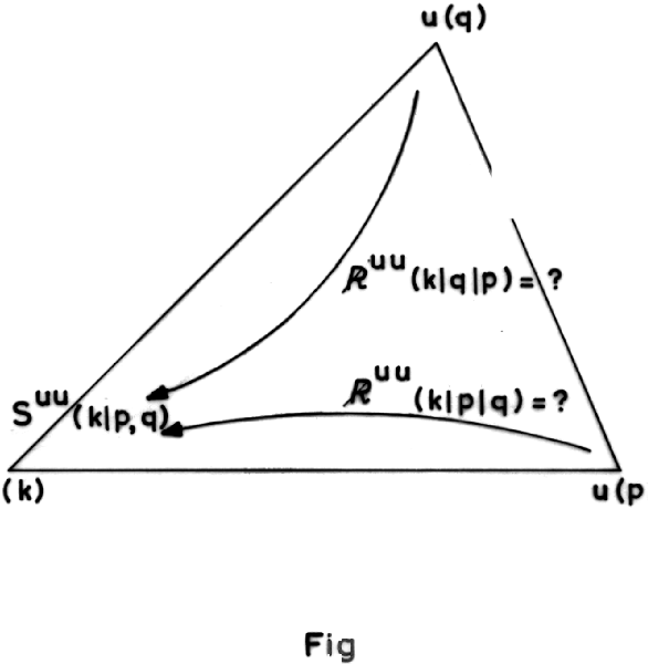
FIG. 2.:

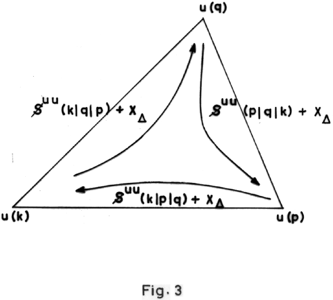
FIG. 3.:

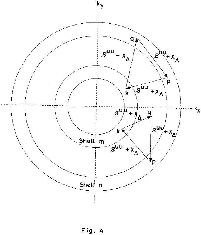
FIG. 4.:

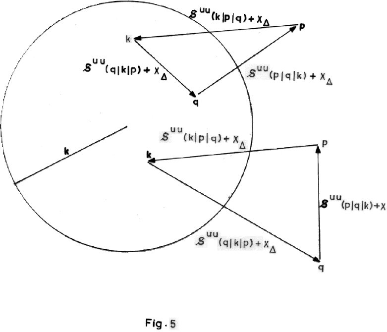
FIG. 5.:

FIG. 6.:

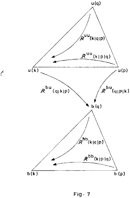
FIG. 7.:

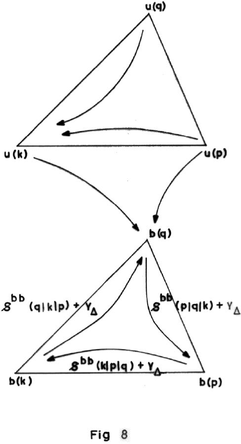
FIG. 8.:

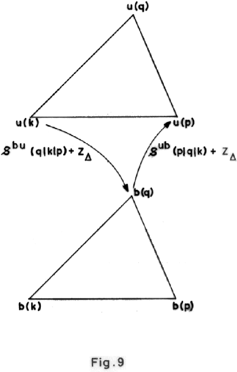
FIG. 9.:

FIG. 10.:

REFERENCES

- [1] J. A. Domaradzki and R. S. Rogallo. Phys. Fluids A, 2:413, 1990.
- [2] J. A. Domaradzki. Phys. Fluids, 31:2747, 1988.
- [3] Y. Zhou. Phys. Fluids A, 5:1092, 1993.
- [4] Y. Zhou. Phys. Fluids A, 5:2511, 1993.
- [5] R. H. Kraichnan. J. Atmos. Sci., 33:1521, 1976.
- [6] J. A. Domaradzki, R. W. Metcalfe, R. S. Rogallo, and J. J. Riley. Phys. Rev. Lett., 58:547, 1987.
- [7] G. K. Batchelor. Proc. Roy. Soc. (London), 2:413, 1950.
- [8] M. K. Verma, D. A. Roberts, M. L. Golstein, S. Ghosh, and W. T. Stribling. J. Geophys. Res., 101:21619, 1996.
- [9] A. Pouquet, U. Frisch, and J. Leorat. J. Fluid Mech., 77:321, 1976.
- [10] A. Pouquet. J. Fluid Mech., 88:1, 1978.
- [11] A. Ishizawa and Y. Hattori. chao-dyn/9810036, 1998.
- [12] A. Ishizawa and Y. Hattori. J. Phys. Soc. Jpn., 67:441, 1998.
- [13] M. Lesieur. Turbulence in Fluids - Stochastic and Numerical Modelling. Kluwer Academic Publishers, 1990.
- [14] D. C. Leslie. Developments in the theory of turbulence. Oxford University Press, 1973.
- [15] R. H. Kraichnan. J. Fluid Mech., 5:497, 1959.
- [16] M. M. Stanisic. The Mathematical Theory of Turbulence. Springer-Verlag, 1985.
- [17] G. Dar, M. K. Verma, and V. Eswaran, (submitted to Phys. Plasma)