Successive approximations for charged particle motion

Abstract

Single particle dynamics in electron microscopes, ion or electron lithographic instruments, particle accelerators, and particle spectrographs is described by weakly nonlinear ordinary differential equations. Therefore, the linear part of the equation of motion is usually solved and the nonlinear effects are then found in successive order by iteration methods.

When synchrotron radiation is not important, the equation can be derived from a Hamiltonian or a Lagrangian. The Hamiltonian nature can lead to simplified computations of particle transport through an optical device when a suitable computational method is used. H. Rose and his school have contributed to these techniques by developing and intensively using the eikonal method [1, 2, 3]. Many ingenious microscopic and lithographic devices were found by Rose and his group due to the simple structure of this method [4, 5, 6].

The particle optical eikonal method is either derived by propagating the electron wave or by the principle of Maupertuis for time independent fields. Maybe because of the time dependent fields which are often required, in the area of accelerator physics the eikonal method has never become popular, although Lagrange methods had been used sometimes already in early days [7]. In this area classical Hamilitonian dynamics is usually used to compute nonlinear particle motion. Here I will therefore derive the eikonal method from a Hamiltonian quite familiar to the accelerator physics community.

With the event of high energy polarized electron beams [8] and plans for high energy proton beams [9], nonlinear effects in spin motion have become important in high energy accelerators. I will introduce a successive approximation for the nonlinear effects in the coupled spin and orbit motion of charged particles which resembles some of the simplifications resulting from the eikonal method for the pure orbit motion.

To H. Rose on the occasion of his 65th birthday

I Introduction

The well known Lagrange variational principle requires

$$\delta\int{\cal L}dt=\delta\int[\vec{\tilde{p}}\cdot\dot{\vec{q}}-{\cal H}]dt=0$$ (1)

with the Lagrangian ${\cal L}$, Hamiltonian ${\cal H}$, and generalized momenta $\vec{\tilde{p}}$ and coordinates $\vec{q}$.

In this principle all variations of $\vec{q}(t)$ are allowed and therefore the Euler–Lagrange equations of motion hold,

$$\frac{d}{dt}\partial_{\dot{\vec{q}}}{\cal L}(\vec{q},\dot{\vec{q}},t)=\partial_{\vec{q}}{\cal L}(\vec{q},\dot{\vec{q}},t)\ .$$ (2)

For relativistic single particle motion the Lagrangian is

$${\cal L}=-mc\sqrt{c^{2}-\dot{\vec{r}}^{2}}+e\dot{\vec{r}}\cdot\vec{A}-e\Phi$$ (3)

where the position $\vec{r}(\vec{q})$ is a function of the generalized coordinates $\vec{q}$. The Jacobian matrix $\underline{r}$ of this function can be written in the form $\underline{r}=(\partial_{\vec{q}}\vec{r}^{T})^{T}$ and has the elements $r_{ij}=\partial_{q_{j}}r_{i}$. In this efficient notation $\vec{r}^{T}$ is the transpose

of the $3\times 1$ matrix $\vec{r}$. The Jacobian matrix of the function $\dot{\vec{r}}(\dot{\vec{q}})$ is also $\underline{r}$ since $\dot{\vec{r}}=\sum_{i=1}^{3}\dot{q_{i}}\partial_{q_{i}}\vec{r}=\underline{r}\dot{\vec{q}}$.

The generalized momentum is $\vec{\tilde{p}}=\partial_{\dot{\vec{q}}}{\cal L}={\underline{r}}^{T}(m\gamma\dot{\vec{r}}+e\vec{A})$ and the variational principle can thus be written as

$$\delta\int[\vec{\tilde{p}}^{T}\underline{r}^{-1}\dot{\vec{r}}-{\cal H}]dt = \delta\int[(m\gamma\dot{\vec{r}}+e\vec{A})^{T}\underline{r}\;\underline{r}^{-1}\dot{\vec{r}}-{\cal H}]dt$$ (4)

$$= \delta\int[m\gamma v^{2}+e\vec{A}^{T}\dot{\vec{r}}-{\cal H}]dt\ .$$ (5)

If only variations $\delta_{{\cal H}=E}$ are considered which keep the total energy ${\cal H}=E$ constant, the variational principle becomes

$$\delta_{{}_{{\cal H}=E}}\int[\vec{\tilde{p}}\cdot\dot{\vec{q}}-{\cal H}]dt = \delta_{{}_{{\cal H}=E}}\int\vec{\tilde{p}}\cdot d\vec{q}$$ (6)

$$=\delta_{{}_{{\cal H}=E}}\int[m\gamma v^{2}+e\vec{A}^{T}\dot{\vec{r}}]dt = 0\ .$$ (7)

The variational principle for constant total energy is called the principle of Maupertuis. However, in equation (7) it does not lead to Euler–Lagrange equations of motion, since not all variations are allowed.

A particle optical device usually has an optical axis or some design curve along which a particle beam should travel. This design curve $\vec{R}(l)$ is parameterized by a variable $l$ and the position of a particle in the vicinity of the design curve has coordinates $x$ and $y$ along the unit vectors $\vec{e}_{x}$ and $\vec{e}_{y}$ in a plane perpendicular this curve. This coordinate system is shown in figure 1. The third coordinate vector $\vec{e}_{l}=d\vec{R}/dl$ is tangential to the design curve and the curvature vector is $\vec{\kappa}=-d\vec{e}_{l}/dl$.

The unit vectors $\vec{e}_{x}$ and $\vec{e}_{y}$ in the usual Frenet–Serret comoving coordinate system rotate with the torsion of the design curve. If this rotation is wound back, the equations of motion do not contain the torsion of the design curve. The position and the velocity are

$$\vec{r}=x\vec{e}_{x}+y\vec{e}_{y}+\vec{R}(l)\ ,\ \ \dot{\vec{r}}=\dot{x}\vec{e}_{x}+\dot{y}\vec{e}_{y}+h\dot{l}\vec{e}_{l}\ ,$$ (8)

with $h=1+x\kappa_{x}+y\kappa_{y}$. This method is described in [3] and [10] and is mentioned here since design curves with torsion are becoming important when considering particle motion in helical wigglers, undulators, and wavelength shifters [11], and for polarized particle motion in helical dipole Siberian Snakes [12].

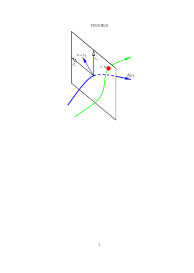
FIG. 1.: Curvatures $\kappa_{x}$, $\kappa_{y}$ of the design curve and generalized coordinates $x$, $y$, and $l$.

The variational principle (7) for the three generalized coordinates $x(t)$, $y(t)$, and $l(t)$ can now be written for the two generalized coordinates $x(l)$ and $y(l)$. This has the following two advantages: a) The particle trajectory along the design curve is usually more important than the particle position at a time $t$, and b) Whereas $\delta_{{}_{{\cal H}=E}}$ does not allow for all variations of the three coordinates, the total energy can be conserved for all variations of the two coordinates $x$ and $y$ by choosing for each position $\vec{r}$ the appropriate momentum with $m\gamma v=\sqrt{(E-e\Phi(\vec{r}))^{2}/c^{2}-(mc)^{2}}$. We obtain from equation (7)

$$\delta_{{}_{{\cal H}=E}}\int\vec{\tilde{p}}\cdot d\vec{q}=\delta\int[m\gamma v^{2}\frac{dt}{dl}+ev\vec{A}\cdot\frac{d\vec{r}}{dl}]dl=0$$ (9)

with $d\vec{r}/dl=x^{\prime}\vec{e}_{x}+y^{\prime}\vec{e}_{y}+h\vec{e}_{l}$ and $dt/dl=|d\vec{r}/dl|/v$. Since all variations are allowed, the integrand is a very simple new Lagrangian

$$\tilde{L}=m\gamma v\sqrt{{x^{\prime}}^{2}+{y^{\prime}}^{2}+h^{2}}+e(x^{\prime}A_{x}+y^{\prime}A_{y}+hA_{l})$$ (10)

which leads to Euler–Lagrange equations of motion

$${\tilde{p}}_{x} = \partial_{x^{\prime}}\tilde{L}\ ,\ \ {{\tilde{p}}_{x}}^{\prime}=\partial_{x}\tilde{L}\ ,$$ (11)

$${\tilde{p}}_{y} = \partial_{y^{\prime}}\tilde{L}\ ,\ \ {{\tilde{p}}_{y}}^{\prime}=\partial_{y}\tilde{L}\ .$$ (12)

The integral $\int_{0}^{l}\tilde{L}(\tilde{l})d\tilde{l}$ is called the eikonal.

Since the Hamiltonian formulation is very common in the area of accelerator physics, we will show how the eikonal can be derived from a Hamiltonian formulation.

The equations of motion for the three generalized coordinates $x(t)$, $y(t)$, and $l(t)$ can be obtained from the Hamiltonian

$${\cal H}=e\Phi+$$ (13)

$$\sqrt{m^{2}c^{2}+({\tilde{p}}_{x}-eA_{x})^{2}+({\tilde{p}}_{y}-eA_{y})^{2}+({\tilde{p}}_{l}/h-eA_{l})^{2}}\ .$$ (14)

In the case of time independent fields, ${\cal H}$ is the conserved total energy $E$ and there are only five independent variables, rather than six. Note that the velocity dependent or non holonomic [13] boundary condition ${\cal H}(\vec{p}(\vec{q},\dot{\vec{q}}),\vec{q},t)=E$ cannot be included in the Lagrange formalism directly. But in the Hamilton formalism this can be done. Furthermore, a switch of independent variable from $t$ to $l$ can easily be done in the Hamiltonian formulation. The Lagrange formulation is therefore abandoned (too easily, as will be shown later). In the variational condition

$$\delta\int[\dot{x}{\tilde{p}}_{x}+\dot{y}{\tilde{p}}_{y}+\dot{l}{\tilde{p}}_{l}-{\cal H}]dt=0$$ (15)

one can change to the independent variable $l$ as follows:

$$\delta\int[x^{\prime}{\tilde{p}}_{x}+y^{\prime}{\tilde{p}}_{y}+(-t^{\prime}){\cal H}-(-{\tilde{p}}_{l})]dl=0\ .$$ (16)

The six canonical coordinates are now $x$, ${\tilde{p}}_{x}$, $y$, ${\tilde{p}}_{y}$, $-t$, and ${\cal H}$, and the new Hamiltonian is given by $\tilde{H}=-{\tilde{p}}_{l}$ which has to be expressed as a function of the six coordinates [14, 15],

$$\tilde{H}=-h{\bigg{[}}eA_{l}+$$ (17)

$$\sqrt{({\cal H}-e\Phi)^{2}-(mc^{2})^{2}-({\tilde{p}}_{x}-eA_{x})^{2}-({\tilde{p}}_{y}-eA_{y})^{2}}{\bigg{]}}\ .$$ (18)

In the Hamilton formalism it is simple to take advantage of the fact that the total energy is conserved for time independent fields; ${\cal H}^{\prime}=\partial_{t}\tilde{H}=0$ leads to ${\cal H}=E$. Then from the six coordinates only the first four have to be considered, leading to the Lagrangian

$$\tilde{L}=x^{\prime}{\tilde{p}}_{x}+y^{\prime}{\tilde{p}}_{y}-\tilde{H}\ .$$ (19)

From $x^{\prime}=\partial_{{\tilde{p}}_{x}}\tilde{H}=\frac{h}{\sqrt{\phantom{h}}}({\tilde{p}}_{x}-eA_{x})$, $y^{\prime}=\partial_{{\tilde{p}}_{y}}\tilde{H}=\frac{h}{\sqrt{\phantom{h}}}({\tilde{p}}_{y}-eA_{y})$ where $\sqrt{\phantom{h}}$ is the square root in $\tilde{H}$ one obtains

$$\sqrt{\phantom{h}} = h\sqrt{\frac{(E-e\Phi)^{2}-(mc^{2})^{2}}{x^{\prime 2}+y^{\prime 2}+h^{2}}}$$ (20)

$$= m\gamma v\frac{h}{\sqrt{x^{\prime 2}+y^{\prime 2}+h^{2}}}\ ,$$ (21)

$${\tilde{p}}_{x} = \frac{\sqrt{\phantom{h}}}{h}x^{\prime}+eA_{x}\ ,\ \ {\tilde{p}}_{y}=\frac{\sqrt{\phantom{h}}}{h}y^{\prime}+eA_{y}\ ,$$ (22)

$$\tilde{L}=m\gamma v\sqrt{{x^{\prime}}^{2}+{y^{\prime}}^{2}+h^{2}}+e(x^{\prime}\!A_{x}+y^{\prime}\!A_{y}+hA_{l})$$ (23)

for $m\gamma v=\sqrt{(E-e\Phi)^{2}/c^{2}-(mc)^{2}}$. The very simple Lagrangian $\tilde{L}$ agrees with the integrand (10) of the eikonal.

In the following it will be shown how the Hamiltonian and the Lagrangian equations of motion for the particle trajectory $\vec{q}(l)$ can be solved in an iterative way. We write a general equation of motion for a coordinate vector $\vec{z}$ in the form

$${\vec{z}}^{\;\prime}=\vec{f}^{1}(\vec{z},l)+\vec{f}^{\geq 2}(\vec{z},l)$$ (24)

where we assume that $\vec{z}=0$ is a solution of the differential equation. Furthermore, we assume $\vec{z}$ to be small and let $\vec{f}^{1}$ be linear in the coordinates. We assume that the nonlinear part of the equation of motion can be expanded in a Taylor series $\vec{f}^{\geq 2}$. The linearized equation of motion is solved by a trajectory $\vec{z}_{1}(l)=\underline{M}(l)\vec{z}_{i}$ which depends linearly on the initial coordinates. For the transport matrix $\underline{M}(l)$ we therefore have

$$\underline{M}^{\prime}\vec{z}_{i}=\underline{f^{1}}\;\underline{M}\vec{z}_{i}$$ (25)

for all coordinate vectors $\vec{z}_{i}$; $\underline{f^{1}}$ being the Jacobian matrix of $\vec{f}^{1}$.

One can write every solution of (24) as $\vec{z}(l)=\underline{M}(l)\vec{\zeta}(l)$, leading to the equation of motion

$$\underline{M}^{\prime}\vec{\zeta}+\underline{M}{\vec{\zeta}}^{\;\prime}=\underline{f^{1}}\underline{M}\vec{\zeta}+\vec{f}^{\geq 2}(\vec{z})\ .$$ (26)

The Taylor coefficients of $\vec{\zeta}(\vec{z}_{i},l)$ with respect to the initial coordinates $\vec{z}_{i}=\vec{\zeta}(0)$ are called aberration coefficients. With equation (25) one obtains

$$\vec{z}(l)=\underline{M}(l)\{\vec{z}_{i}+\int_{0}^{l}{\underline{M}}^{-1}(\tilde{l})\vec{f}^{\geq 2}(\vec{z}(\tilde{l}))\}d\tilde{l}\ .$$ (27)

Now we assume that the general solution $\vec{z}(\vec{z}_{i},l)$ can be expanded in a power series with respect to the initial coordinates. Then symbolizing the $j$th order Taylor polynomial with $[\ldots]_{j}$, we write the orders up to $j$ as $\vec{z}_{j}=[\vec{z}(\vec{z}_{i},l)]_{j}$, i.e. we use lower indices to describe the order of $\vec{z}_{i}$. The upper index in $\vec{f}$ describes the order in $\vec{z}$, which is in turn a nonlinear function of $\vec{z}_{i}$. When $\vec{z}_{n-1}$ is known, one can iterate the expansion up to order $n$ with equation (27), since

$$\vec{z}_{n}=\underline{M}(l)\{\vec{z}_{i}+\int_{0}^{l}{\underline{M}}^{-1}(\tilde{l})[\vec{f}^{\geq 2}(\vec{z}_{n-1})]_{n}\}d\tilde{l}\ .$$ (28)

The zeroth order of the expansion with respect to the coordinates must vanish, which means that the trajectory $\vec{q}=0$ must satisfy the equation of motion for some momentum $p(l)$. Additionally we require that the vector potential on the design curve is gauged to zero. This can always be achieved. The canonical momentum $\vec{p}$ then also vanishes for the trajectory $\vec{q}=0$. It then follows that the Hamiltonian and the Lagrangian have no components linear in the coordinates and momenta. When computing trajectories through a particle optical device, it is customary to normalize the momenta to the initial design momentum $p_{0}=p(0)$. The following two dimensional generalized coordinates are therefore used:

$$\vec{q} = {x\choose y}\ ,\ \ \vec{p}={{\tilde{p}}_{x}/p_{0}\choose{\tilde{p}}_{y}/p_{0}}\ ,$$ (29)

$$L(\vec{q},{\vec{q}}^{\;\prime},l) = \tilde{L}/p_{0}\ ,\ \ \vec{p}=\partial_{{\vec{q}}^{\;\prime}}L\ ,\ \ {\vec{p}}^{\;\prime}=\partial_{\vec{q}}L\ ,$$ (30)

$$H(\vec{q},\vec{p},l) = \tilde{H}/p_{0}\ ,\ \ {\vec{q}}^{\;\prime}=\partial_{\vec{p}}H\ ,\ \ {\vec{p}}^{\;\prime}=-\partial_{\vec{q}}H\ .$$ (31)

The Euler–Lagrange equations lead to the second order differential equations $\frac{d}{dl}\partial_{{\vec{q}}^{\;\prime}}L=\partial_{\vec{q}}L$ for the two dimensional vector $\vec{q}$.

II Successive approximation in terms of Hamiltonians

In the Hamilton formalism one obtains first order equations of motion for the four dimensional vector $\vec{z}^{T}=(q_{1},q_{2},p_{1},p_{2})$. With the antisymmetric matrix $\underline{J}$ one can write the equation of motion as

$$\underline{J}=\left(\begin{array}[]{rr}{\underline{0}}_{2}&{\underline{1}}_{2}\\ -{\underline{1}}_{2}&{\underline{0}}_{2}\end{array}\right)\ ,\ \ {\vec{z}}^{\;\prime}=\underline{J}\partial_{\vec{z}}H\ ,$$ (32)

with the $2\times 2$ identity and zero matrixes ${\underline{1}}_{2}$ and ${\underline{0}}_{2}$. This structure implies special symmetries for the transport maps $\vec{\cal M}$ of particle optics. These maps describe how the final phase space coordinates $\vec{z}_{f}=\vec{\cal M}(\vec{z}_{i})$ of a particle, after flying through an optical device, are related to the initial coordinates $\vec{z}_{i}$. These maps are often weakly nonlinear and can be expanded in a Taylor expansion. The Hamiltonian nature implies that the Jacobian $\underline{\cal M}=(\partial_{\vec{z}}\vec{\cal M}^{T})^{T}$ of any transport map $\vec{\cal M}(\vec{z})$ is symplectic [13], meaning that

$$\underline{\cal M}\;\underline{J}\;\underline{\cal M}^{T}=\underline{J}\ .$$ (33)

For the successive approximations we separate the equation of motion into its linear and nonlinear part,

$${\vec{z}}^{\;\prime}=\underline{J}\partial_{\vec{z}}(H^{2}+H^{\geq 3})\ .$$ (34)

After we have solved for the linear transport matrix $\vec{z}_{1}=\underline{M}\vec{z}_{i}$, we can iterate by equation (28) which takes the form

$$\vec{z}_{n}=\underline{M}\{\vec{z}_{i}+\int_{0}^{l}{\underline{M}}^{-1}[\underline{J}\partial_{\vec{z}}H^{\geq 3}(\vec{z}_{n-1})]_{n}d\tilde{l}\}$$ (35)

With the relation $\underline{\cal M}^{-1}\;\underline{J}=\underline{J}\;\underline{\cal M}^{T}$ from equation (33) this can be written as

$$\vec{z}_{n}=\underline{M}\{\vec{z}_{i}+\underline{J}\int_{0}^{l}{\underline{M}}^{T}[\partial_{\vec{z}}H^{\geq 3}(\vec{z}_{n-1})]_{n}d\tilde{l}\}\ .$$ (36)

The corresponding equation for the aberrations ${\vec{\zeta}}_{n}={\underline{M}}^{-1}{\vec{z}}_{n}$ becomes

$$\vec{\zeta}_{n}=\vec{z}_{i}+\underline{J}\int_{0}^{l}[\partial_{\vec{\zeta}}H^{\geq 3}(\underline{M}\vec{\zeta}_{n-1})]_{n}d\tilde{l}\ .$$ (37)

This form of the iteration equation is quite simple. However, since the Hamiltonian (17) is a complicated function, the evaluation of the four integrals can become very cumbersome.

III Successive approximation in terms of Lagrangians

In [3] Rose used a variational principle to derive a successive approximation to nonlinear motion based on the eikonal. This method iterates position $\vec{q}$ and momentum $\vec{p}$ in their nonlinear dependence on the initial position ${\vec{q}}_{i}$ and momentum $\vec{p}_{i}$. Knowing the order $n-1$ dependence ${\vec{q}}_{n-1}$ and $\vec{p}_{n-1}$, one has to compute ${\vec{q}}^{\;\prime}_{n-1}$ by differentiation of ${\vec{q}}_{n-1}$ or by inversion of $\vec{p}=\partial_{{\vec{q}}^{\;\prime}}L(\vec{q},{\vec{q}}^{\;\prime},l)$. Then the eikonal can be evaluated to compute the order $n$ dependence ${\vec{q}}_{n}$ and $\vec{p}_{n}$. In general it can be cumbersome to compute ${\vec{q}}^{\;\prime}_{n-1}$ and therefore here we derive a new version of the eikonal method, which iterates directly ${\vec{q}}^{\;\prime}_{n}$ rather than the momentum.

In deriving the simple form of equation (37), advantage has only been taken of the symplectic first order transfer matrix. We therefore wish to exploit this advantage again by working with new coordinates which are identical with the canonical $\vec{q}$ and $\vec{p}$ up to first order so that the new coordinates lead to the same first order transport matrix $\underline{M}$. To first order one obtains

$$\vec{p}=\partial_{{\vec{q}}^{\;\prime}}L=\frac{p(s)}{p_{0}}{\vec{q}}^{\;\prime}+\frac{e}{p_{0}}{A_{x}^{1}\choose A_{y}^{1}}+{\cal O}^{2}(\vec{q},{\vec{q}}^{\;\prime})$$ (38)

where $p(s)$ is the momentum of a particle traveling on the design curve $\vec{q}=0$, and the upper index 1 specifies the part of the vector potential linear in $x$ and $y$. We therefore work with the coordinates

$$\vec{Q}={\vec{q}\choose\vec{u}}={{\vec{q}}\choose{\frac{p(s)}{p_{0}}{\vec{q}}^{\;\prime}+\frac{e}{p_{0}}{{A_{x}^{1}}\choose{A_{y}^{1}}}}}\ .$$ (39)

Moreover, it can be shown [16, 3, 17, 18] that the contribution from the vector potential can be gauged to vanish whenever there is no longitudinal magnetic field $B_{0}{\vec{e}}_{l}$ on the design curve. Then if one investigates trajectories which start with momentum $p_{0}$ in a region free of such a field, we have the simple relation $\vec{u}_{i}={\vec{q}}^{\;\prime}_{i}$.

By splitting the Lagrangian into its second order and its higher order part, the equation of motion becomes

$${\vec{Q}}^{\;\prime} = {\vec{q}\choose\vec{u}}^{\prime}$$ (40)

$$= {\frac{p_{0}}{p(s)}\vec{u}-\frac{e}{p(s)}{A_{x}^{1}\choose A_{y}^{1}}\choose\partial_{\vec{q}}L^{2}}-{0\choose\frac{d}{d\tilde{l}}\partial_{{\vec{q}}^{\;\prime}}L^{\geq 3}-\partial_{\vec{q}}L^{\geq 3}}\ .$$ (41)

After having solved the linearized equation of motion, we obtain with equation (28)

$$\vec{Q} = \underline{M}\{{\vec{Q}}_{i}-\int_{0}^{l}\underline{M}^{-1}{0\choose\frac{d}{d\tilde{l}}\partial_{{\vec{q}}^{\;\prime}}L^{\geq 3}-\partial_{\vec{q}}L^{\geq 3}}d\tilde{l}\}$$ (42)

$$= \underline{M}\{{\vec{Q}}_{i}+\underline{J}\int_{0}^{l}\underline{M}^{T}{\frac{d}{d\tilde{l}}\partial_{{\vec{q}}^{\;\prime}}L^{\geq 3}-\partial_{\vec{q}}L^{\geq 3}\choose 0}d\tilde{l}\}\ .$$ (43)

An integration by parts leads to

$$\vec{Q} = \underline{M}\{{\vec{Q}}_{i}-\underline{J}\int_{0}^{l}[{\underline{M}^{\prime}}^{T}{\partial_{{\vec{q}}^{\;\prime}}L^{\geq 3}\choose 0}+{\underline{M}}^{T}{\partial_{\vec{q}}L^{\geq 3}\choose 0}]d\tilde{l}$$ (45)

$$+\underline{J}{\bigg{[}}{\underline{M}}^{T}{\partial_{{\vec{q}}^{\;\prime}}L^{\geq 3}\choose 0}{\bigg{]}}_{0}^{l}\}\ .$$

Writing the Jacobian as ${\underline{M}}^{T}=\partial_{{\vec{Q}}_{i}}{\vec{Q}}_{1}^{T}=\partial_{{\vec{Q}}_{i}}(\vec{Q}-{\vec{Q}}_{\geq 2})^{T}$ where $\vec{Q}={\vec{Q}}_{1}+{\vec{Q}}_{\geq 2}$ was split into parts which depend on ${\vec{Q}}_{i}$ linearly and nonlinearly, we obtain

$${\underline{M}}^{-1}\vec{Q}={\vec{Q}}_{i}-\underline{J}\int_{0}^{l}[(\partial_{{\vec{Q}}_{i}}({\vec{q}}^{\;\prime T}-{\vec{q}}_{\geq 2}^{\;\prime T}))\partial_{{\vec{q}}^{\;\prime}}L^{\geq 3}$$ (46)

$$+(\partial_{{\vec{Q}}_{i}}({\vec{q}}^{T}-{\vec{q}}_{\geq 2}^{T}))\partial_{\vec{q}}L^{\geq 3}]d\tilde{l}+\underline{J}{\bigg{[}}(\partial_{{\vec{Q}}_{i}}{\vec{q}}_{1}^{T})\partial_{{\vec{q}}^{\;\prime}}L^{\geq 3}{\bigg{]}}_{0}^{l}$$ (47)

$$={\vec{Q}}_{i}-\underline{J}\int_{0}^{l}[\partial_{{\vec{Q}}_{i}}L^{\geq 3}-(\partial_{{\vec{Q}}_{i}}{\vec{q}}_{\geq 2}^{\;\prime T})\partial_{{\vec{q}}^{\;\prime}}(L-L^{2})$$ (48)

$$-(\partial_{{\vec{Q}}_{i}}{\vec{q}}_{\geq 2}^{T})\partial_{\vec{q}}(L-L^{2})]d\tilde{l}+\underline{J}{\bigg{[}}(\partial_{{\vec{Q}}_{i}}{\vec{q}}_{1}^{T})\partial_{{\vec{q}}^{\;\prime}}L^{\geq 3}{\bigg{]}}_{0}^{l}$$ (49)

$$={\vec{Q}}_{i}-\underline{J}\int_{0}^{l}[\partial_{{\vec{Q}}_{i}}L^{\geq 3}+(\partial_{{\vec{Q}}_{i}}{\vec{q}}_{\geq 2}^{\;\prime T})\partial_{{\vec{q}}^{\;\prime}}L^{2}+(\partial_{{\vec{Q}}_{i}}{\vec{q}}_{\geq 2}^{T})\partial_{\vec{q}}L^{2}$$ (50)

$$-(\partial_{{\vec{Q}}_{i}}{\vec{q}}_{\geq 2}^{\;\prime T})\partial_{{\vec{q}}^{\;\prime}}L-(\partial_{{\vec{Q}}_{i}}{\vec{q}}_{\geq 2}^{T})\frac{d}{d\tilde{l}}\partial_{{\vec{q}}^{\;\prime}}L]d\tilde{l}$$ (51)

$$+\underline{J}{\bigg{[}}(\partial_{{\vec{Q}}_{i}}{\vec{q}}_{1}^{T})\partial_{{\vec{q}}^{\;\prime}}L^{\geq 3}{\bigg{]}}_{0}^{l}\ .$$ (52)

Note that the $A^{\prime}_{x}$, $A^{\prime}_{y}$, $p(s)$ and $p_{0}$ of equation (39) drop out of the right hand side of equation (52) owing to the multiplications by the zeros in equation (45). The second order $L^{2}$ of the Lagrangian is a quadratic form in which every quadratic combination of the $\vec{q}$ and ${\vec{q}}^{\;\prime}$ can occur. It can be written using a matrix $\underline{L^{2}}$ as $L^{2}={\vec{Q}}^{T}\underline{L^{2}}\vec{Q}$. Part of the above integrand can be rewritten as

$${\vec{q}}_{\geq 2}^{\;\prime T}\partial_{{\vec{q}}^{\;\prime}}L^{2}+{\vec{q}}_{\geq 2}^{T}\partial_{\vec{q}}L^{2}={\vec{Q}}_{\geq 2}^{T}\underline{L^{2}}\vec{Q}+{\vec{Q}}^{T}\underline{L^{2}}{\vec{Q}}_{\geq 2}\ .$$ (53)

For convenience we write $L^{2}(\vec{a})={\vec{a}}^{T}\underline{L^{2}}\vec{a}$. Another integration by parts in equation (52) leads to

$${\underline{M}}^{-1}\vec{Q} = {\vec{Q}}_{i}-\underline{J}\int_{0}^{l}[\partial_{{\vec{Q}}_{i}}(L^{\geq 3}+L^{2}({\vec{Q}}_{\geq 2}))$$ (56)

$$+(\partial_{{\vec{Q}}_{i}}{\vec{q}}_{\geq 2}^{\;\prime T})\partial_{{\vec{q}}^{\;\prime}_{1}}L^{2}({\vec{Q}}_{1})+(\partial_{{\vec{Q}}_{i}}{\vec{q}}_{\geq 2}^{T})\partial_{{\vec{q}}_{1}}L^{2}({\vec{Q}}_{1})]d\tilde{l}$$

$$+\underline{J}{\bigg{[}}(\partial_{{\vec{Q}}_{i}}{\vec{q}}_{\geq 2}^{T})\partial_{{\vec{q}}^{\;\prime}}L+(\partial_{{\vec{Q}}_{i}}{\vec{q}}_{1}^{T})\partial_{{\vec{q}}^{\;\prime}}L^{\geq 3}{\bigg{]}}_{0}^{l}\ .$$

The first part of the integral contains $L_{E}=L^{\geq 3}+L^{2}({\vec{Q}}_{\geq 2})$. The integral $\int_{0}^{l}L_{E}d\tilde{l}$ is called the perturbation eikonal. This scheme embodies the essential requirement that the $n+1$ order dependence of $L_{E}$ on the initial variables $\vec{Q}_{i}$ can be computed already when $Q_{n-1}$ is known; $\vec{Q}_{n}$ does not need to be known. For an iteration of ${\vec{Q}}_{n}$, knowledge of ${\vec{Q}}_{n-1}$ is sufficient. Since ${\vec{q}}_{1}$ satisfies the first order equation of motion, we can use the relation $\partial_{{\vec{q}}_{1}}L^{2}({\vec{Q}}_{1})=\frac{d}{dl}\partial_{{\vec{q}}^{\;\prime}_{1}}L^{2}({\vec{Q}}_{1})$ to perform another integration by parts,

$${\underline{M}}^{-1}\vec{Q} = {\vec{Q}}_{i}-\underline{J}\partial_{{\vec{Q}}_{i}}\int_{0}^{l}L_{E}d\tilde{l}+\underline{J}{\bigg{[}}(\partial_{{\vec{Q}}_{i}}{\vec{q}}_{\geq 2}^{T})\partial_{{\vec{q}}^{\;\prime}}L$$ (58)

$$+(\partial_{{\vec{Q}}_{i}}{\vec{q}}_{1}^{T})\partial_{{\vec{q}}^{\;\prime}}L^{\geq 3}-(\partial_{{\vec{Q}}_{i}}{\vec{q}}_{\geq 2}^{T})\partial_{{\vec{q}}^{\;\prime}_{1}}L^{2}({\vec{Q}}_{1}){\bigg{]}}_{0}^{l}$$

$$= {\vec{Q}}_{i}-\underline{J}\partial_{{\vec{Q}}_{i}}\int_{0}^{l}L_{E}d\tilde{l}+\underline{J}{\bigg{[}}(\partial_{{\vec{Q}}_{i}}{\vec{q}}^{T})\partial_{{\vec{q}}^{\;\prime}}L$$ (60)

$$-(\partial_{{\vec{Q}}_{i}}{\vec{q}}_{1}^{T})\partial_{{\vec{q}}^{\;\prime}}L^{2}-(\partial_{{\vec{Q}}_{i}}{\vec{q}}_{\geq 2}^{T})\partial_{{\vec{q}}^{\;\prime}_{1}}L^{2}({\vec{Q}}_{1}){\bigg{]}}_{0}^{l}\ .$$

$\partial_{{\vec{Q}}_{i}}L_{E}$ is the part of $\partial_{{\vec{Q}}_{i}}L$ which up to order $n$ in ${\vec{Q}}_{i}$ does not depend on ${\vec{Q}}_{n}$. Similarly the term outside the integral is simply the part of $(\partial_{{\vec{Q}}_{i}}{\vec{q}}^{T})\partial_{{\vec{q}}^{\;\prime}}L$ which up to order $n$ does not depend on ${\vec{Q}}_{n}$. We therefore write $(\partial_{{\vec{Q}}_{i}}{\vec{q}}^{T})\partial_{{\vec{q}}^{\;\prime}}L-(\partial_{{\vec{Q}}_{i}}{\vec{q}}_{1}^{T})\partial_{{\vec{q}}^{\;\prime}}L^{2}-(\partial_{{\vec{Q}}_{i}}{\vec{q}}_{\geq 2}^{T})\partial_{{\vec{q}}^{\;\prime}_{1}}L^{2}({\vec{Q}}_{1})=\{(\partial_{{\vec{Q}}_{i}}{\vec{q}}^{T})\partial_{{\vec{q}}^{\;\prime}}L\}_{E}$. If we now express the Lagrangian in terms of the aberrations $\vec{\xi}$ with $\vec{Q}=\underline{M}\vec{\xi}$, we obtain the iteration equation

$${\vec{\xi}}_{n}=_{n}{\vec{Q}}_{i} - \underline{J}\partial_{{\vec{Q}}_{i}}\int_{0}^{l}L_{E}(\underline{M}\vec{\xi}_{n-1})d\tilde{l}$$ (61)

$$+ \underline{J}{\bigg{[}}\{(\partial_{{\vec{Q}}_{i}}{\vec{q}}^{T})\partial_{{\vec{q}}^{\;\prime}}L\}_{E}{\bigg{]}}_{0}^{l}\ .$$ (62)

When computing ${\vec{\xi}}_{n}$ from ${\vec{\xi}}_{n-1}$ with this iteration equation, all parts of the right hand side which contribute to higher orders are neglected, as indicated by $=_{n}$. This iteration equation can have several advantages over the Hamiltonian iteration equation (28):

• The Lagrangian (10) is a much simpler function than the Hamiltonian (17).

• The derivative in equation (61) is performed after the integral has been evaluated. Therefore only one integral has to be computed and it describes all four coordinates of ${\vec{\xi}}_{n}$.

• The fact that the various coordinates are the derivatives with respect to initial conditions yields very simple relations [19] between the various expansion coefficients of ${\vec{\xi}}_{n}$, which are the so called aberration coefficients of particle optical devices. These relations can be much simpler than relations entailed by the symplectic symmetry implicit in the Hamiltonian formulation.

• The second pair of coordinates in equation (39) can be calculated very easily. With equations (26) and (40), the equation of motion for $\vec{\xi}$ is

  $$\underline{M}{\vec{\xi}}^{\;\prime}={0\choose\frac{d}{d\tilde{l}}\partial_{{\vec{q}}^{\;\prime}}L^{\geq 3}-\partial_{\vec{q}}L^{\geq 3}}\ .$$ (63)

  After having computed ${\vec{q}}_{n}=\vec{M}_{2\times 4}{\vec{\xi}}_{n}$ by iteration, the derivative ${\vec{q}}^{\;\prime}$ can then easily be computed as ${\vec{q}}^{\;\prime}_{n}={\vec{M}}^{\;\prime}_{2\times 4}{\vec{\xi}}_{n}$ using equation (63). One thus only needs to iterate the two dimensional vector ${\vec{q}}_{n}$ and not a four dimensional vector ${\vec{z}}_{n}$ as in the Hamiltonian iteration procedure.

IV Successive approximation for spin orbit motion

The time variation of a spin $\vec{s}$ in the rest frame of a particle is described by the so called Thomas–BMT equation $\dot{\vec{s}}=\vec{\Omega}_{BMT}\times\vec{s}$ [20, 21] where

$$\vec{\Omega}_{BMT}= - \frac{q}{m\gamma}\{(a\gamma+1)\vec{B}_{\perp}+(1+a)\vec{B}_{\|}$$ (64)

$$- \frac{\gamma}{c}\vec{\beta}\times\vec{E}(a+\frac{1}{1+\gamma})\}$$ (65)

with the electric field $\vec{E}$, the parts of the magnetic field $\vec{B}$ which are perpendicular ($\perp$) and parallel ($\|$) to the particle’s velocity, and the anomalous gyro-magnetic factor $a=\frac{g-2}{2}$.

Changing to the comoving coordinate system of figure (1), we obtain $\vec{s}=S_{x}\vec{e}_{x}+S_{y}\vec{e}_{y}+S_{l}\vec{e}_{l}$ and ${\vec{s}}^{\;\prime}=(S^{\prime}_{x}-S_{l}\kappa_{x})\vec{e}_{x}+(S^{\prime}_{y}-S_{l}\kappa_{y})\vec{e}_{y}+(S^{\prime}_{l}+S_{x}\kappa_{x}+S_{y}\kappa_{y})\vec{e}_{l}$. The equation of motion for the vector $\vec{S}$ of these spin components is then

$${\vec{S}}^{\;\prime} = \vec{\Omega}\times\vec{S}\ ,$$ (66)

$$\vec{\Omega} = \vec{\Omega}_{BMT}\frac{h}{v}\sqrt{x^{\prime 2}+y^{\prime 2}+h^{2}}-\vec{\kappa}\times\vec{e}_{l}\ .$$ (67)

The equations of motion for the phase space vector $\vec{z}$ and the spin $\vec{S}$ have the form

$${\vec{z}}^{\;\prime}=\vec{f}(\vec{z},l)\ ,\ \ {\vec{S}}^{\;\prime}=\vec{\Omega}(\vec{z},l)\times\vec{S}\ .$$ (68)

The general solutions transporting the coordinates along the optical system, starting at the initial values $\vec{z}_{i}$, $\vec{S}_{i}$, is given by the transport map ${\cal M}$ and the rotation matrix $\underline{R}\in SO(3)$,

$$\vec{z}(l)=\vec{\cal M}(\vec{z}_{i},l)\ ,\ \ \vec{S}(l)=\underline{R}(\vec{z}_{i},l)\vec{S}_{i}\ .$$ (69)

In order to find the general solution, one could compute the nine coefficients of the rotation matrix by solving the differential equation

$$R_{ij}(\vec{z}_{i},l)^{\prime}=\epsilon_{ilk}\Omega_{l}R_{kj}(\vec{z}_{i},l)\ ,$$ (70)

where the vector product was expressed by the totally antisymmetric tensor $\epsilon_{ilk}$. However, computing the nine components of the rotation matrix seems inefficient, since a rotation can be represented by three angles. It has turned out [22] to be most efficient to represent the rotation of spins by the quaternion $A$ which gives the rotation transformation in the SU(2) representation as

$$A=a_{0}\underline{1}-{\rm i}\vec{a}\cdot\vec{\underline{\sigma}}\ .$$ (71)

Here $\underline{1}$ is the $2\times 2$ identity matrix and the elements of the vector $\vec{\underline{\sigma}}$ are the three two dimensional Pauli matrixes. When a rotation by an angle $\phi$ is performed around the unit vector $\vec{e}$, the quaternion representation of the rotation has $a_{0}=\cos(\phi/2)$ and $\vec{a}=\sin(\phi/2)\vec{e}$. Therefore $a_{0}^{2}+{\vec{a}}^{2}=1$ and the identity transformation is represented by $a_{0}=1$.

If a particle traverses an optical element which rotates the spin according to the quaternion $A$ and then passes through an element which rotates the spin according to the quaternion $B$, the total rotation of the spin is given by

$$C = c_{0}\underline{1}-{\rm i}\vec{c}\cdot\vec{\underline{\sigma}}=(b_{0}\underline{1}-{\rm i}\vec{b}\cdot\vec{\underline{\sigma}})(a_{0}\underline{1}-{\rm i}\vec{a}\cdot\vec{\underline{\sigma}})$$ (72)

$$= (b_{0}a_{0}-\vec{b}\cdot\vec{a})\underline{1}-{\rm i}(b_{0}\vec{a}+\vec{b}a_{0}+\vec{b}\times\vec{a})\cdot\vec{\underline{\sigma}}\ .$$ (73)

The concatenation of quaternions can be written in matrix form as

$$\vec{C} = {c_{0}\choose\vec{c}}=\underline{B}{a_{0}\choose\vec{a}}\ ,$$ (74)

$$\underline{B} = \left(\begin{array}[]{rrrr}b_{0}&-b_{1}&-b_{2}&-b_{3}\\ b_{1}&b_{0}&-b_{3}&b_{2}\\ b_{2}&b_{3}&b_{0}&-b_{1}\\ b_{3}&-b_{2}&b_{1}&b_{0}\end{array}\right)\ .$$ (79)

This concatenation of two quaternions can be used to find a differential equation for the spin rotation.

While propagating along the design curve by a distance $dl$, spins are rotated by an angle $\Omega dl=|\Omega|dl$ around the vector $\vec{\Omega}$. After having been propagated to $l$ by the quaternion $A$, a spin gets propagated from $l$ to $l+dl$ by the quaternion with $b_{0}=1$ and $\vec{b}=\frac{1}{2}\vec{\Omega}dl$. The resulting total rotation is given by $A+A^{\prime}dl$ and we obtain the differential equation

$${a_{0}^{\prime}\choose\vec{a}^{\;\prime}}=\frac{1}{2}\left(\begin{array}[]{rrrr}0&-\Omega_{1}&-\Omega_{2}&-\Omega_{3}\\ \Omega_{1}&0&-\Omega_{3}&\Omega_{2}\\ \Omega_{2}&\Omega_{3}&0&-\Omega_{1}\\ \Omega_{3}&-\Omega_{2}&\Omega_{1}&0\end{array}\right){a_{0}\choose\vec{a}}\ .$$ (80)

Writing the matrix as $\underline{\Omega}$ and the vector as $\vec{A}$, the spin orbit equation of motion has the form

$${\vec{z}}^{\;\prime}=\vec{f}(\vec{z},l)\ ,\ \ \vec{A}^{\prime}=\underline{\Omega}(\vec{z},l)\vec{A}\ .$$ (81)

The starting conditions are $\vec{z}(0)=\vec{z}_{0}$, $a_{0}=1$, and $\vec{a}=0$. The quaternion $A$ depends on the initial phase space coordinates $\vec{z}_{i}$ and can be expanded in a Taylor series with respect to these coordinates. In the following we want to devise an iteration method for $A_{n}$, which is the Taylor expansion to order $n$ of $A$.

The rotation vector $\vec{\Omega}$ is split into its value on the design curve and its phase space dependent part as $\vec{\Omega}(\vec{z},l)=\vec{\Omega}^{0}(l)+\vec{\Omega}^{\geq 1}(\vec{z},l)$. The spin motion on the design curve is given by $\vec{A}^{\prime}_{0}(l)=\underline{\Omega}^{0}\vec{A}_{0}(l)$. Similarly to equation (26), spin aberrations are defined with respect to the leading order motion. Small phase space coordinates will create a rotation which differs little from $\vec{A}_{0}(l)$ and we write the phase space dependent rotation as a concatenation of $\vec{A}_{0}$ and the $\vec{z}$ dependent rotation $(1+\delta,\vec{\delta})$ which reduces to the identity for $\vec{z}=0$ by requiring that the aberrations $\delta$ and $\vec{\delta}$ vanish on the design curve. With equation (74) we obtain

$$\vec{A}=\underline{A_{0}}{1+\delta\choose\vec{\delta}}\ .$$ (82)

The quaternion $A$ is now inserted in the differential equation (81) to obtain

$$\underline{A}^{\prime}_{0}{1+\delta\choose\vec{\delta}} + \underline{A}_{0}{\delta^{\prime}\choose{\vec{\delta}}^{\prime}}$$ (83)

$$= (\underline{\Omega}^{0}+\underline{\Omega}^{\geq 1})\underline{A}_{0}{1+\delta\choose\vec{\delta}}\ .$$ (84)

Taking into account the equation on the design curve and the fact that $\underline{A}_{0}^{T}$ describes the inverse rotation of $\underline{A}_{0}$, we obtain

$${\delta^{\prime}\choose{\vec{\delta}}^{\prime}}=(\underline{A}_{0}^{T}\underline{\Omega}^{\geq 1}\underline{A}_{0}){1+\delta\choose{\vec{\delta}}}=\underline{\tilde{\Omega}}(\vec{z},l){1+\delta\choose{\vec{\delta}}}\ .$$ (85)

Writing the Taylor expansion to order $n$ in $\vec{z}_{i}$ one finally obtains the iteration equation

$${\delta_{n}\choose{\vec{\delta}}_{n}}=_{n}\int_{0}^{l}\underline{\tilde{\Omega}}(\vec{z}_{n}){1+\delta_{n-1}\choose{\vec{\delta}}_{n-1}}d\tilde{l}\ ,\ \ {\delta_{0}\choose\vec{\delta}_{0}}=0\ .$$ (86)

This iteration method was used for the spin transport in the program SPRINT [22] and was evaluated using MATHEMATICA in [23].

In the case of successive approximation in terms of the Hamiltonian, the various aberration coefficients were related by the symplectic symmetry. With the Lagrange formalism the various aberration coefficients were related by their being derivatives of a common integral with respect to different initial coordinates. In the case of the successive approximation for spin motion, the various aberration coefficients in $\vec{\delta}$ and $\delta$ are related by the relation $(1+\delta)^{2}+\vec{\delta}^{2}=0$.

Acknowledgment

I owe thanks to D. Barber, H. Mais, and M. Vogt for thoroughly reading the manuscript and for the resulting improvements.

REFERENCES

[1]
H. Rose and U. Petri.
Optik, 33:151, 1971.
[2]
E. Plies and D. Typke.
Dreidimensional abbildende Eledtronenmikroskope II. Theorie
elektronenoptischer Systeme mit gekrümmter Achse.
Zeitschrift für Naturforschung, 33a, 1361-1377, 1978.
[3]
H. Rose.
Hamiltonian magnetic optics.
Nuclear Instruments and Methods in Physics Research,
A258:374–401, 1987.
[4]
H. Rose.
Correction of aperture aberrations in magnetic systems with threefold
symmetry aberration.
Nuclear Instruments and Methods 187, 187-199, 1981.
[5]
H. Rose.
Outline of a spherically corrected semiaplanatic medium-voltage
transmission electron microscope.
Optic, 85(1):19–24, 1990.
[6]
H. Rose, M. Haider, and K. Urban.
Elektronenmikroskopie mit atomarer Auflösung.
Physikalische Blätter, 54(5):411–416, 1998.
[7]
P. A. Sturrock.
Static and dynamic electron optics, Part II.
Cambridge University Press, p. 149, 1995.
[8]
D. P. Barber, et al.
The first achievement of longitudinal spin polarization in a high
energy electron storage ring.
Physics Letters, B(343):436–443, 1995.
[9]
SPIN Collaboration and the DESY Polarization Team.
Acceleration of polarized protons to 820 GeV at HERA.
UM–HR 96–20, University of Michigan Report, 1996.
[10]
G. H. Hoffstätter.
Nonlinear dependence of synchrotron radiation on beam parameters.
In Proceedings of PAC 94, Dallas/TX, 1995.
[11] G. Wüstefeld.
Orbit maps for
helical snake and helical undulator magnets.
In Proceedings of the workshop “Polarized Protons at High Energies”,
DESY, Hamburg, 1999.
[12]
A. Luccio and T. Roser.
Third workshop on Siberian Snakes and spin rotators.
formal report BNL-52453, Brookhaven National Laboratory, Upton, New
York, 1994.
[13]
H. Goldstein.
Classical Mechanics.
Addison-Wesley, Reading/MA, USA, 1980.
Second edition.
[14]
E. D. Courant and H. S. Snyder.
Theory of the alternating–gradient synchrotron.
Annals of physics, 3:1–48, 1958.
[15]
H. Mais.
Some topics in beam dynamics of storage rings.
formal report DESY 96–119, DESY, 1996.
[16]
E. Plies and H. Rose.
Über die axialen Bildfehler magnetischer Ablenksysteme mit
krummer Achse.
Optik 34, 2, 171-190, 1971.
[17]
G. Hoffstätter.
Geometrische Elektronenoptik angewandt auf ein durch Hexapole
korrigiertes Mikroskop mit sub Ångström Auflösung.
Master’s thesis, Darmstadt University of Technology, 1991.
[18]
G. H. Hoffstätter and H. Rose.
Gauge invariance in the eikonal method.
Nuclear Instruments and Methods in Physics Research,
A328:398–401, 1993.
[19]
G. H. Hoffstaetter.
Comments on aberration correction in symmetric imaging energy
filters.
Nuclear Instruments and Methods in Physics Research, page
accepted, 1998.
[20]
L. H. Thomas.
Phil. Mag., 3:1, 1927.
[21]
V. Bargmann, L. Michel, and V. L. Telegdi.
Precession of the polarization of particles moving in a homogeneous
electromagnetic field.
Physical Review Letters, 2(10):435–436, 1959.
[22]
K. Heinemann and G. H. Hoffstätter.
A tracking algorithm for the stable spin polarization field in
storage rings using stroboscopic averaging.
Physical Review E, 54:4240–4255, 1996.
and official DESY Report 96–078.
[23]
Ch. Weißbäcker.
Nichtlineare Effekte der Spindynamik in
Protonenbeschleunigern.
Master’s thesis, Darmstadt University of Technology, 1998.