An inertial range length scale in structure functions.

Abstract

It is shown using experimental and numerical data that within the traditional inertial subrange defined by where the third order structure function is linear that the higher order structure function scaling exponents for longitudinal and transverse structure functions converge only over larger scales, $r>r_{S}$, where $r_{S}$ has scaling intermediate between $\eta$ and $\lambda$ as a function of $R_{\lambda}$. Below these scales, scaling exponents cannot be determined for any of the structure functions without resorting to procedures such as extended self-similarity (ESS). With ESS, different longitudinal and transverse higher order exponents are obtained that are consistent with earlier results. The relationship of these statistics to derivative and pressure statistics, to turbulent structures and to length scales is discussed.

1 Introduction

An important tool in understanding intermittency in turbulence has been the exponents $\zeta_{p}$ of power laws for the velocity structure functions. The longitudinal structure functions are

$$S^{L}_{p}(r)=<(u(x+r)-u(x))^{p}>\sim r^{\zeta^{L}_{p}}$$ (1)

where $\overrightarrow{u}$ and $\overrightarrow{r}$ are in the same direction. Their measurement requires only a single hot wire probe that can, through the Taylor frozen turbulence assumption, determine one velocity component $u$ as a function of the parallel spatial direction $r$ and thus find the $S^{L}_{p}$ at high Reynolds numbers. Using crossed-wire probes, one can also obtain reliable, high Reynolds number measurements of transverse structure functions $S^{T}_{p}(r)$, where $\overrightarrow{u}$ and $\overrightarrow{r}$ are orthogonal, and their exponents $\zeta^{T}_{p}$. There are also mixed structure functions containing both longitudinal and transverse components.

The relationship between the $\zeta_{p}$ and intermittency [1] is in deviations of the the exponents $\zeta_{p}$ from their Gaussian or classical values of $\zeta_{p}=p/3$, where $\zeta_{2}\approx 2/3$ and $\zeta_{3}=1$ are expected for an energy cascade. In the presence of intermittency, $\zeta_{p}<p/3$ for $p>3$ is expected. Furthermore, it has generally been believed that all of the $\zeta^{L,T}_{p}$ of a given order $p$ should be the same in the infinite Reynolds number limit. This is closely related to the refined similarity hypothesis (RSH) which assumes that the only information that can affect the statistics on a given scale $r$ is the fluctuations in the energy cascade $\epsilon_{r}$ through that scale. Details about either the large scale forcing or the dissipative structures should be irrelevant in this picture. Measurements [2] have confirmed RSH as it relates dissipation to longitudinal statistics.

More recently, moderate Reynolds numbers simulations and experiments [3, 4] have found, with the help of the extended self-similarity hypothesis [5], that $\zeta^{T}_{p}~{}<~{}\zeta^{L}_{p}$ for $p>3$. This has been now been confirmed over all Reynolds numbers simulated [6] or observed [7] to date. If longitudinal and transverse statistics are different, then the statistics of strain, that is dissipation $\epsilon_{r}$, and the statistics of of vorticity, call it $\Omega_{r}$ for its relationship to the enstrophy, should be different. Since $\zeta^{T}_{p}~{}<~{}\zeta^{L}_{p}$, it implies that vorticity is more intermittent than strain. This possibility has been suggested by recent numerical results [6] that show that dissipation and enstrophy statistics scale as RSH predicts, but with separate distributions. This result implies that when the nonlinear coupling is written as a convolution in Fourier space that not only the velocity magnitude, but also the velocity phase, what makes the transfer of $\Omega_{r}$ different than $\epsilon_{r}$, is important. Related to this, if the dissipation-dissipation correlation and its $\Omega_{r}$ counterpart go as

$$<\epsilon_{x}\epsilon_{x+r}>~{}\sim~{}r^{\mu}\quad{\rm and}<\Omega_{x}\Omega_{x+r}>~{}\sim~{}r^{\mu^{\Omega}}$$ (2)

then different $\Omega_{r}$ statistics implies that $\mu^{\Omega}\neq\mu$. Experimentally, $\mu\approx 0.25$ [21] has been confirmed by the latest measurements and simulations [22, 10, 8], although lower Reynolds number measurements tend to give $\mu=0.5$. $\mu^{\Omega}\neq\mu$ is found in one numerical result [8].

It will be shown here that different longitudinal and transverse statistics suggest the existence of a crossover length scale within the inertial subrange. That is a length scale distinct from the large length scale $L$ or a multiple of the dissipation or Kolmogorov scale $\eta$, and maybe the order of the intermediate Taylor microscale $\lambda$, where the Taylor microscale Reynolds number and $\lambda$ are defined as

$$R_{\lambda}={{U\lambda}\over\nu}\quad\quad{\rm where}\quad\lambda={U\over{<(du/dx)^{2}.>^{1/2}}}$$ (3)

$R_{\lambda}$ is the definition of the Reynolds number that appears to give uniform scaling in a variety of different flows and is related to the large scale Reynolds number by $R_{\lambda}\sim(R=UL/\nu)^{1/2}$. The Kolmogorov scale is related to $\lambda$ by

$$\eta=(\nu/\epsilon)^{1/4}\sim\lambda R_{\lambda}^{-1/2}$$ (4)

where $\nu$ is viscosity and $\epsilon$ is the dissipation rate.

In order to discern if there is some crossover length scale for some structure function within the inertial subrange and determine if there are indeed different longitudinal and transverse exponents, a long inertial subrange and clean data are needed. Numerical simulations do not have this range, but if run sufficiently long give clean data and more flexibility. Observations can provide more dynamic range, but with more limited types of data. This paper will use both experimental and numerical data to try to present a more complete picture than either measurements or simulations alone of what evidence there is for different longitudinal and transverse statistics and its implications. Experimental data will be used to indicate the high Reynolds number trends, then analysis from forced numerical turbulence in a box at $R_{\lambda}=262$ on a $512^{3}$ mesh and $R_{\lambda}=390$ on a $1024^{3}$ mesh will be presented, with most of the discussion related to the $R_{\lambda}=262$ calculation. It will be shown that if the same inertial range scaling analysis defined by the experiments is applied to the simulations, then the trends in the lower Reynolds number simulations are consistent with the experiments and clearly demonstrate a trend where simple scaling breaks down at many multiples of the Kolmogorov scale within the traditional inertial subrange, and that this scale appears to increase with Reynolds number.

This paper will be organized as follows. First, constraints on and relationships between structure functions will be discussed. Recent results on structure function and pressure structure function scaling will be discussed in the context that different scalings for the same order imply the existence of a statistically signficant length scale within the inertial subrange where scaling properties of at least some structure functions could change. Next, there will be a discussion of existing experimental and observational results before showing new analysis of experimental data up to $R_{\lambda}=3200$. The analysis will use $S_{2}^{L,T}$ and $S_{3}$ to define the minimum limits over which inertial subrange scaling analysis can be applied before the results for the $\zeta^{L,T}_{p}$ for $p=4$ and 6 are presented. Then the numerical analysis will be presented in a similar manner.

2 Constraints

This section discusses kinematical constraints upon structure functions, related quantities, and what can be measured. There are only a few hard constraints for the scaling of small $p$ structure functions. For $p=2$, assuming isotropy and homogeniety and for a long enough inertial subrange, $\zeta^{L}_{2}=\zeta^{T}_{2}$ is expected. The classical value for $\zeta_{2}$ is 2/3 (5), which is closely related to assuming that the energy spectrum goes as

$$E(k)=c_{k}\epsilon^{2/3}k^{-5/3}$$ (5)

where $c_{K}$ is the experimentally determined Kolmogorov constant and $\epsilon$ is the equivalently either the rate of energy dissipation or the rate of energy transfer to small scales. With crossed wires, only one-dimensional longitudinal or transverse spectra can be found, but with a numerical simulation the full energy spectrum can be obtained in three-dimensions. An example from the $512^{3}$ forced data set to be discussed is shown in Figure 1. This spectrum is found between a lower wavenumber, large-scale, forcing or integral scale $L$ and a high wavenumber, small-scale, dissipation scale $\eta=(\nu/\epsilon)^{1/4}$, with $k_{\eta}=1/\eta$.

Figure 1: Three-dimensional kinetic energy spectrum $E(|k|)$ for the $512^{3}$ forced calculation. The dashed line has an exponent of -5/3 and $k_{\eta}=k_{\max}=256$. The dissipation spectrum $\epsilon(k)=\nu k^{2}E(k)$ with a peak at $k=34$ is shown. Resolution is determined by the ratio of the wavenumber of the peak of the dissipation spectrum (here $k\approx k_{\eta}/30=34$) to $k_{\max}$. Experience has shown that a ratio of at least 5 provides adequate resolution.

The theoretical basis for predicting a -5/3 spectrum is the presumption of a local, uniform energy cascade. There is no constraint requiring -5/3 or the corresponding $\zeta_{2}=2/3$ for structure functions and corrections to the $\zeta_{2}=2/3$ are claimed [9]. However, no corrections to a -5/3 energy spectrum have been seen in numerical spectrum such as Figure 1 and for the largest range of scales observationally [10]. How could two supposedly equivalent measures of turbulent scaling, the energy spectrum and the 2nd order structure functions, yield two inconsistent results concerning intermittency? A suggestion below is that dissipation range effects on $S^{L}_{2}$ are more persistent than thought.

For $p=3$, by balancing transfer and dissipation terms in the Karman-Howarth equation [11, 12], $\zeta_{3}\equiv 1$ is expected. This is the only fixed constraint on the $\zeta_{p}$ for isotropic, homogeneous turbulence regardless of intermittency and yields Kolmogorov’s 4/5 law for $S_{3}(r)$

$$S_{3}(r)=-{4\over 5}\epsilon r$$ (6)

However, linear in $r$ behavior is never observed exactly (see discussion with figure 2). This effect has been quantified [13] and it was shown that the peak of $-S_{3}/r$, after being compensated for the effects of forcing and dissipation, has a Reynolds number dependence like $l_{s}/L\sim R_{\lambda}^{-3/5}$, whereas $\lambda/L\sim R_{\lambda}^{-1}$. This could suggest the existence of a dynamically significant position in the inertial subrange that does not scale with either the small Kolmogorov scale or the large scale and has been interpreted in terms of an enstrophy production argument [14].

While it is difficult to obtain a clean power law for $p=3$, it is even harder to get convincing power laws when plotting $S_{p}$ versus $r$ for $p>3$. A device that has been used to determine higher order $\zeta_{p}$ is to make the assumption that even if $-S_{3}\sim r$ is not exact, if it is assumed to be exact then much stronger power laws for the $S_{p}$, $p\geq 4$, can be obtained by plotting $S_{p}$ versus $-S_{3}$ rather than versus $r$. This is known as extended self-similarity or ESS [5]. Another way of looking at ESS is that the $S_{p}$ are not true power laws all the way to the dissipation scale $\eta$, but only for $r>A\eta$, where $A$ is large, and ESS allows one to extend scaling much closer to $\eta$. However, there is a question of how much of this is a mirage because the ESS scaling exponents as $r\rightarrow 0$ are trivially the classical values of $p/3$. The additional length scale $A\eta$ probably should have no dynamical significance since it is a multiple of $\eta$, as will be discussed in section 3.

For $p\geq 4$, there are no rigorous constraints that the longitudinal and transverse structure functions should have the same $\zeta_{p}$. However, it has been shown [15] that when all components of the velocity field $\overrightarrow{u}$ and all directions of $\overrightarrow{\partial_{x}}$ are considered that there are four rotationally invariant combinations of fourth-order derivative correlations that can be written entirely in terms of the strain $e_{ij}$ and the vorticity $\omega_{i}$ and have been discussed in detail [16].

$$F_{e}=(15/7){{<(e^{2})^{2}>}\over{<e^{2}>^{2}}}\quad\quad F_{e\omega}=3{{<\omega^{2}e^{2}>}\over{<\omega^{2}><e^{2}>}}$$ (7)

$$F_{\omega ee\omega}=3{{<\omega_{i}e_{ij}e_{jk}\omega_{k}>}\over{<\omega^{2}><e^{2}>}}\quad\quad F_{\omega}=(9/5){{<\omega^{4}>}\over{<\omega^{2}>^{2}}}$$

Under the assumptions of homogeneity and isotropy $F_{e}$ is equivalent to the longitudinal fourth-order derivative flatness $F_{4}^{L}$ that can be measured with a single hot-wire probe and is related to the $r\rightarrow 0$ limit of $S_{4}^{L}(r)$. To determine the other irrotational flatnesses as functions of $R_{\lambda}$ can only be done at low Reynolds numbers with complicated probes [17] or simulations [16, 18], which suggest that each has its own scaling with Reynolds number.

With a crossed-wire probe, higher Reynolds number observations of the scaling of flatnesses related to the $r\rightarrow 0$ limit of the transverse and mixed structure functions could be determined. In addition to

$$F^{L}_{4}=F_{\ell\ell\ell\ell}=<u_{1,1}^{4}>/<u_{1,1}^{2}>^{2}=F_{e}$$ (8)

these are

$$F^{M}_{4}=F_{\ell\ell tt}={{<u_{1,1}^{2}u_{2,1}^{2}>}\over{<u_{1,1}^{2}><u_{2,1}^{2}>}}$$ (9)

and

$$F^{T}_{4}=F_{tttt}={{<u_{2,1}^{4}>}\over{<u_{2,1}^{2}>^{2}}}$$ (10)

which can be related to combinations of the irrotational flatnesses (7). The scaling of $F^{M}_{4}$ and $F^{T}_{4}$ should be dominated by their most intermittent components, which the analysis of the irrotational components indicates is $F_{\omega}$ [16].

Generalized structure functions should involve not only more than one velocity direction, but also more than one spatial position and direction. All of the structure functions discussed so far involve different velocity components, but only one spatial position and direction. In this class would be included structure functions where the angle between $\overrightarrow{u}$ and $\overrightarrow{\partial_{x}}$ is not 0 or $90^{\circ}$ [19]. The different rotationally invariant flatnesses (7) involve different velocity and spatial directions, but only one position, $r=0$. It should be noted that a new type of structure function that uses two spatial positions in the same direction, has recently come into use in conjunction with fusion models [20]. These are similar to the dissipation-dissipation correlation functions $<\epsilon_{x}\epsilon_{x+r}>$ where the two distances would be 0 (the derivative for dissipation) and the separation $r$ between the two locations of dissipation $\epsilon$.

While generalized structure functions could only be completely determined by numerical simulations or complicated probes at low Reynolds numbers, some insight might be gained by considering whether their number could be reduced. First, a way of systematically writing these down is needed [24]. However, unlike the way all fourth order derivative correlations can be expressed in terms of just four irrotational correlations, no simple reduction to a small number of fourth order structure functions has been found. What can be said is that if this number could be reduced, it would have to satisfy two rotational groups, one for position and the other for the velocity components [25]. The full group would correspond to the spin plus angular momentum group in quantum mechanics. Even if such a reduction does not exist, one would expect some general properties to hold among all fourth-order structure functions. For example, if there is a subrange where the longitudinal and transverse structure functions, $S_{4}^{L}(r)$ and $S_{4}^{T}(r)$, do have the same scaling, then maybe all fourth-order structure functions, including those related to fusion rules, are related in a similar manner. Or if there is a subrange where $S_{4}^{L}(r)$ and $S_{4}^{T}(r)$, do not have the same scaling, then relationships such as the fusion rules should not apply.

This leads us to three fourth-order structure functions measurable with crossed wire probes, each corresponding to one of the three derivative flatnesses (8-10). The longitudinal, mixed and transverse fourth-order structure functions are

$$S^{L}_{4}=S_{\ell\ell\ell\ell}=<(u(x+r)-u(x))^{4}>$$

$$S^{M}_{4}=S_{\ell\ell tt}=<(u(x+r)-u(x))^{2}(v(x+r)-v(x))^{2}>$$ (11)

$$S^{T}_{4}=S_{tttt}=<(v(x+r)-v(x))^{4}>$$

whose general moment form is given by eqns. 13.83-13.84 of [26]. However, the general moment form in no more fundamental than (11) in terms of the full rotational group. One would expect that if there are different scalings for the derivative flatnesses (7) under $R_{\lambda}$, there should also be correspondingly different $\zeta^{L,M,T}_{p}$, with $\zeta^{M}_{p}$ and $\zeta^{T}_{p}$ more strongly dominated by the vorticity statistics.

3 Why two length scales?

Another way of looking at the fourth-order velocity structure functions is to consider the second order pressure structure function $P_{2}(r)$. This is related to a combination of fourth-order velocity structure functions (11) by [27]

$$P_{2}(r)=<(p(x+r)-p(x))^{2}>=-{1\over 3}S^{L}_{4}(r)+{4\over 3}r^{2}\int_{r}^{\infty}y^{-3}[S^{L}_{4}(y)+S^{T}_{4}(y)-6S^{M}_{4}(y)]dy$$ (12)

$$+{4\over 3}\int_{0}^{r}y^{-1}[S^{T}_{4}(y)-3S^{M}_{4}(y)]dy$$

Assuming $S^{L}_{4}(r)\sim\zeta_{4}^{L}$,$S^{T}_{4}(r)\sim\zeta_{4}^{T}$, and $S^{M}_{4}(r)\sim\zeta^{M}_{4}$ then

$$P_{2}(r)=-{1\over 3}(1+{4\over{2-\zeta_{4}^{L}}})S_{4}^{L}(r)+{4\over 3}({1\over\zeta_{4}^{T}}-{1\over{2-\zeta_{4}^{T}}})S_{4}^{T}(r)$$

$$-4({1\over\zeta^{M}_{4}}-{2\over{2-\zeta^{M}_{4}}})S^{M}_{4}(r)$$

For the purposes here, the particular numerical prefactors are not important. The point to be made is that if the fourth-order longitudinal and transverse structure functions have different scalings, then $P_{2}$ should have different scaling at the two ends of the inertial subrange. Assume that $S^{L}_{4}\sim r^{\zeta^{L}_{4}}$ and $S^{T}_{4}\sim r^{\zeta^{T}_{4}}$ with $\zeta^{L}_{4}>\zeta^{T}_{4}$ and the scaling for $S^{M}_{4}$ between these. Then for $r$ small, $P_{2}$ would be dominated by the scaling of $S^{T}_{4}$ and for large $r$ by $S^{L}_{4}$, with some crossover length scale in the middle of the inertial subrange marking the separation between two regimes for the scaling of $P_{2}$.

Related to $P_{2}(r)$ is the pressure spectrum $S_{p}(k)$. It has been suggested [28] that the dependence of $P_{2}(k)$ on the spectral equivalents of the dissipation-dissipation correlation function $<\epsilon_{x}\epsilon_{x+r}>$ and also $<\Omega_{x}\Omega_{x+r}>$ and a cross correlation $<\Omega_{x}\epsilon_{x+r}>$ places a kinematical constraint upon exponents for these correlations, and therefore the related fourth-order velocity structure functions. The relation used to show this is

$$S_{p}(k)={{\epsilon^{2}}\over{4k^{4}\nu^{2}}}[E^{\epsilon}(k)+E^{\Omega}(k)-E^{M}(k)]$$ (13)

where $E^{\epsilon}(k)$, $E^{\Omega}(k)$, and $E^{M}(k)$ are the spectral versions of $<\epsilon_{x}\epsilon_{x+r}>$, $\nu^{2}<\Omega_{x}\Omega_{x+r}>$, and $\nu<\Omega_{x}\epsilon_{x+r}>$ respectively. If each goes as

$$E^{\epsilon}(k)=C^{\epsilon}\epsilon^{2}k^{-1}(kL)^{-\mu^{\epsilon}}$$ (14)

with corresponding $\mu^{\Omega}$ and $\mu^{M}$ for $E^{\Omega}(k)$ and $E^{M}(k)$, it is then argued that unless $\mu^{\epsilon}=\mu^{\Omega}=\mu^{M}$ for all $k$ there will be divergences in $S_{p}(k)$ as $\nu\rightarrow 0$. This is a reasonable conclusion for $k\rightarrow 0$. However, for $k>k_{\lambda}\sim 1/\lambda$ where $k_{\lambda}^{4}\nu^{2}\sim O(1)$, there is no need for this requirement. Therefore, there could be a kinematical constraint for $0<k<k_{\lambda}$ requiring that $\mu^{\epsilon}=\mu^{\Omega}=\mu^{x}$. Relating this to physical space, there would be a constraint that $\zeta^{L}=\zeta^{T}=\zeta^{M}$ as $r\longrightarrow 0$ and $R_{\lambda}\longrightarrow\infty$. This will be shown to be consistent with the analysis in sections (4,5). For $k_{\lambda}<k<k_{\eta}$, there would be no constraint, so that it would be possible that $\mu^{\epsilon}\neq\mu^{\Omega}\neq\mu^{M}$ and $\zeta^{L}\neq\zeta^{T}\neq\zeta^{M}$ as $r\longrightarrow\eta$, which is also indicated by the analysis here. What would be most satisfying would be if the pressure spectrum itself showed a clear break near $k=1/\lambda$. This has now been found in the pressure analysis of the $1024^{3}$ data to be discussed here [29].

4 New experimental evidence

There have been numerous experimental and observation studies of turbulence designed to determine the scaling of structure functions and related measures of intermittency such as the dissipation-dissipation correlation function (2). However, careful examination raises several questions. First, while the highest Reynolds number observations [7] do find that $\zeta^{T}(p)\neq\zeta^{L}(p)$, when ESS is used, compared with lower Reynolds number results, the difference is noticeably less. This suggests that in the very high Reynolds number limit the difference could go to zero. On the other hand, ESS might be giving a false impression of good scaling since the ratios $S^{T}_{p}(r)/S^{L}_{p}(r)$ as functions of $r$ do not show good scaling behavior to as small a scale as plotting with ESS does. A recurrent limitation is that scales below $\lambda$ in experimental and observational analysis are usually not shown, perhaps because it is felt that the small scales are less reliable. For example, the dissipation-dissipation correlation function exponent is expected to be $\mu\approx 0.25$ from the observed value of $\zeta^{L}_{6}\approx 1.78$. This is confirmed by several high Reynolds number measurements ([10, 22] and references therein), but only for $r\geq\lambda$. It is noted [22] that lower $R_{\lambda}$ experiments tend to give $\mu\approx 0.5$. One moderate Reynolds number ($R_{\lambda}=400$) experiment for a circular jet [23] that shows $\mu\approx 0.2$ for $r\geq\lambda$, also shows a breakdown in scaling of $<\epsilon_{x}\epsilon_{x+r}>$ for $r<\lambda$ that could be with the origin of $\mu\approx 0.5$ at low $R_{\lambda}$.

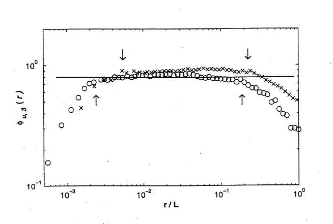
Figure 2: The normalized third-order velocity structure functions. $\phi_{u,3}=-<\Delta u_{r}^{3}>/(<\epsilon>r).$ $\times$, ML; $\circ$, RC. The vertical down and up arrows indicate the classical inertial-range bounds ($r_{\eta}$ and $r_{L}$) for ML and RC, respectively. The isotropic value of $\overline{\phi_{u,3}(r)}=0.8$ is shown by the solid line.

The new experimental analysis comes from data from two experiments at the Moscow wind tunnel that has been used to investigate a number of fundamental issues involving turbulent spectra and structure functions [10, 30]. The two experiments are for a mixing layer ML at $R_{\lambda}$=2100 and a return channel RC at $R_{\lambda}$=3200, which are the highest Reynolds number laboratory data sets available with both longitudinal and transverse velocities. The advantage of an experiment over atmospheric observations is that an experiment offers more controlled conditions, which could be especially important for determining transverse structure functions since any inherent anisotropy in the flow could affect their values. With respect to this, an important point to remember in the following discussion is that the ML data set is very anisotropic and RC data set is nearly completely isotropic. Therefore, only the RC, $R_{\lambda}=3200$ experimental data can be directly compared to the isotropic numerical data to be presented. The ML data set is included to show that most of the relevant properites also appear when there is anisotropy. Extended self-similarity will not be used in order to emphasize the regimes with simple scaling and where this breaks down within the inertial subrange. It will be shown that the scalings of all of the measured higher-order structure functions change within the inertial subrange.

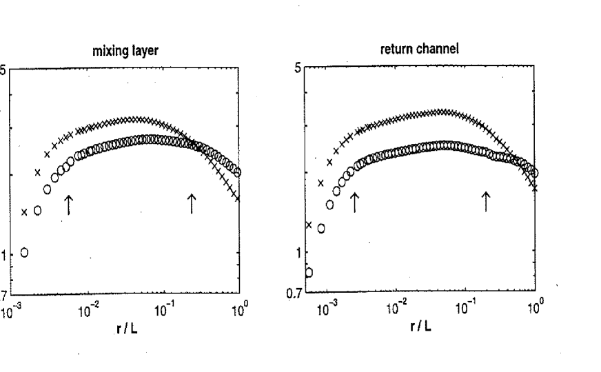
Figure 3: The normalized second-order velocity structure functions. $\phi^{L,T}_{s,2}=<\Delta s_{r}^{2}>/(<\epsilon>r)^{2/3}.$ $\circ,~{}s=u,~{}\phi_{u,2}=\phi^{L}_{2}$; $\times,~{}s=w,~{}\phi_{w,2}=\phi^{T}_{2}$. $\eta=0.00018$ and $0.00014$ for ML and RC respectively. Arrows are $r_{\eta}$ and $r_{L}$. The vertical arrows indicate the classical inertial-range bounds.

Figure 2 shows the third-order longitudinal structure functions $-S_{3}(r)$ divided by $r$ for ML and RC. Excluding using the absolute value, all odd order transverse-only structure functions are zero. Figure 2 uses arrows to indicate the inertial subrange based upon the regime over which $-S_{3}(r)/r$ is constant for ML and RC. For ML and RC respectively, at the large scale arrows are lengths $r_{L}=L/5$ and $L/6$ and at the small scales lengths $r_{\eta}=30\eta$ and $25\eta$. Figure 3 shows the second-order longitudinal $S^{L}_{2}(r)$ and transverse $S^{T}_{2}(r)$ structure functions for ML and RC. For $S^{L}_{2}(r)$, at large $r$ there is scaling out to an $r_{L}$ consistent with $r_{L}$ from $S_{3}(r)$ in Figure 2. In addition, there is a new large length that we will call $r_{4/3}<r_{L}$ over which the isotropic relation $S^{T}_{2}(r)\approx(4/3)S^{L}_{2}(r)$ holds. $r_{4/3}$ is smaller than the range over which the longitudinal second order structure function $S^{L}_{2}$ has good scaling behavior, which is roughly out to $r_{L}$, but is consistent with the maximum $r$ for which the transverse second order structure function $S^{T}_{2}$ has good scaling. For ML and RC, $r_{4/3}=L/30$ and $L/25$ respectively. The small length scale $r_{\eta}$ is roughly where the one must begin to apply extended self-similarity, ESS, (section 2) if one is to get good scaling relationships for the higher order longitudinal structure functions down to the Kolmogorov scale $\eta$. The reason $r_{\eta}$ is being introduced is to clearly indicate that any new length scale between $r_{\eta}$ and $r_{4/3}$ or $r_{L}$ is fully within the inertial subrange. While $r_{4/3}<r_{L}$ at large scales, the range over which the 4/3 rule for $S^{L,T}_{2}(r)$ seems to fit at small scales extends to $r<r_{\eta}$. This would be consistent with how extended self-similarity extends scaling regimes more into the dissipation regime.

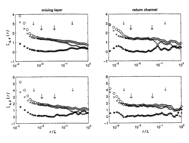
Figure 4: The local slopes $\zeta^{L,T}_{p}(r)=d\log[S^{L,T}_{p}(r)]/d\log(r),\quad p=4,6.$ $s=u$ for $\zeta^{L}_{p}$ and $s=w$ for $\zeta^{T}_{p}$. $\circ,~{}\zeta_{u,p}(r)=\zeta^{L}_{p}(r)$; $\times,~{}\zeta_{w,p}(r)=\zeta^{T}_{p}(r)$; $*,~{}R_{p}(r)=S^{L}_{p}(r)/S^{T}_{p}(r)$. The outer small vertical arrows indicate the classical inertial range bounds, $r_{\eta}$ and $r_{L}$, while the inner large vertical arrows indicated the new bounds, $r_{S}$ and $r_{4/3}$, where $\zeta^{T}_{p}\approx\zeta^{L}_{p}$.

Figures 4(a-d) plot the logarithmic derivatives of the fourth and sixth-order longitudinal and transverse structure functions. For fourth and higher order structure functions there are no isotropy relationships that would require that $S^{T}_{p}$ have the same scaling as $S^{L}_{p}$ over the entire inertial subrange, only the pressure spectum argument (section 3) that $\zeta^{T}_{4}$ should equal $\zeta^{L}_{4}$ for $r>\lambda$. Consistent with the pressure spectrum argument, there is a regime in Figures 4(a-d) where the higher order structure functions do have the same scaling, between two lengths, $r_{4/3}$ and a new small length scale that we will call $r_{S}>r_{\eta}$. Referring to Table 1 for ML ($R_{\lambda}\approx 2100$) and RC ($R_{\lambda}\approx 3200$), $r_{S}=60\eta$ and $50\eta$ respectively while $\lambda=R_{\lambda}^{1/2}\eta\approx 46\eta$ and $56\eta$ respectively. So $r_{S}\approx\lambda$, but it is also roughly twice the value of $r_{\eta}$. For $r<r_{S}$, both $\zeta^{T}_{p}$ and $\zeta^{L}_{p}$ increase rapidly from their $r>r_{S}$ constant values, with $\zeta^{L}_{p}$ increasing the fastest.

This analysis shows a regime within even the rather strict definition of a measurable inertial subrange defined by $r_{\eta}<r<r_{4/3}$ where universal scaling of longitudinal and transverse structure functions is found and therefore assumptions of refined self-similarity might apply. In addition, there is a regime for $r<r_{S}$ where both the longitudinal and transverse scaling exponents diverge from constant behavior. Praskovsky’s analysis shows that if scaling functions were fitted over the entire inertial subrange, that different exponents for the longitudinal and transverse structure functions would be found that would be consistent with recent experiments [7] and simulations [3, 6].

5 New numerical evidence

To determine more clearly how significant the differences between the longitudinal and transverse structure functions are, it is necessary to see some trends. For this purpose we now move to analysis of a $512^{3}$ forced calculation of isotropic turbulence in a periodic box with $R_{\lambda}=262$ and another $1024^{3}$ calculation with $R_{\lambda}=390$. The cleaner numerical data also allows one to more directly compare $S^{L}_{2}$ and $S^{T}_{2}$ and to apply extended self-similarity.

The simulations are classic turbulence simulations in a periodic box with the lowest band of wavenumber modes forced to have constant energy by Gaussian white noise. Statistics were taken several eddy turnover times after any large excursions in the dissipation due to the initial conditions have dissappeared and once the dissipation rate had settled to the point where it was varying by less than 5% on the timescale of several eddy turnover times. Experience has shown that this type of Gaussian white noise forcing yields stable statistics over a single eddy turnover time. The $512^{3}$ simulations were not dealiased and the statistics represent an average over 40 large scale eddy turnover times done on the Cray T3D of the IDRIS Institute in Orsay, France. The $1024^{3}$ calculations were done on a Fujitsu VOO5999/56 at the Nagoya University Compution Center and represent an average over 1.1 large scale eddy turnover times. How well the $1024^{3}$ calculation satisfies isotropy relations for $S^{L,T}_{2}(r)$ and $S_{3}(r)$ is discussed elsewhere [31]. Figure 1 is the three-dimensional kinetic energy spectrum for the $512^{3}$ calculation, showing a clear -5/3 regime. The Kolmogorov scale $\eta$ is half the mesh size $\eta=\Delta x/2$. This is considered adequate resolution because the peak of the dissipation spectrum, roughly where the -5/3 regime rolls over into the dissipation regime, is at $k\approx k_{\eta}/30$ where $k_{\eta}=2\pi/\eta$.

In the experiments above, the original definition of an inertial subrange placed the smallest scale useful for analysis at about $r_{\eta}=25\eta$, roughly the scale associated with the peak of the dissipation spectrum. This definition of $r_{\eta}$ would make it greater than $\lambda$ for both simulations, which for $R_{\lambda}=262$ is $\lambda\approx 16\eta$ and for $R_{\lambda}=390$ is $\lambda\approx 20\eta$. Therefore, a quantitative means of choosing $r_{\eta}$ must be determined that can be applied equally to simulations at lower Reynolds number and the $R_{\lambda}=3200$ experiments. A difficulty in choosing a method is that the simulations are not at high enough a Reynolds number to exhibit either a clearly defined linear regime in $S_{3}$ or a long regime where the isotropy relationship between $S_{2}^{L}$ and $S_{2}^{T}$ is obeyed.

The problem is illustrated by Figure 5, which plots $-S_{3}(r)/(.8\epsilon r)$ and the normalized form with the viscous correction

$$D_{LLL}(r)=\frac{-S_{3}(r)+6\nu{{\partial S_{2}^{L}(r)}\over{\partial r}}}{.8\epsilon r}\quad.$$ (15)

While the span over which $D_{LLL}(r)$ is 1 indicates that there is an energy cascade, an inertial subrange over which $-S_{3}(r)/.8r$ is flat as in the experiments in Figure 2 is not seen. Therefore, arbrtrarily a inertial subrange will be chosen as those $r$ where $-S_{3}(r)/(.8\epsilon r)~{}>~{}0.8$. This is the consistent with how $r_{\eta}$ was chosen for the RC experiment and gives consistent values of $r_{\eta}$ for the $512^{3}$ and $1024^{3}$ simulations and the RC experiment. Based upon Figure 5, an inertial subrange can be defined between $r/\eta=$19 and 193.

Figure 5: $-S_{3}(r)/(.8\epsilon r)$. Also shown is $(-S_{3}(r)+6\nu\partial S_{2}^{L}(r)/\partial r)/(.8\epsilon r)$. An arbitrary constant line is drawn to indicate where an inertial subrange is defined. $r$ is with respect to the size of the box $(2\pi)^{2}$

Let us now use $S^{L}_{2}(r)$ and $S^{T}_{2}(r)$ to consider this definition of an inertial subrange using the isotropic relationship in 3D between the transverse and longitudinal structure functions.

$$S^{T}_{2}(r)=S^{L}_{2}(r)+{r\over 2}\partial S^{L}_{2}(r)/\partial r$$ (16)

In the inertial subrange where $S_{2}(r)\sim r^{2/3}$, from (16) one gets $S^{T}_{2}(r)\sim(4/3)S^{L}_{2}(r)$. As $r\rightarrow 0$, $S_{2}(r)\sim r^{2}$, so one gets $S^{T}_{2}(r)\sim 2S^{L}_{2}(r)$. Figure 6 shows the second-order longitudinal and transverse structure functions divided by $r^{2/3}$. $S^{T}_{2}(r)/r^{2/3}$ is plotted twice, first divided by 4/3 to demonstrate how well the inertial range relation is obeyed and then divided by 2 to demonstrate the approach to the dissipation range.

The 4/3 rule in Figure 6 is only approached at the largest scales, for $r$ greater than where $-S_{3}(r)/(.8\epsilon r)$ is greatest in Figure 5, which could be called $r_{\max}$. For $r<r_{\max}$ in Figure 6, the gradient of $S^{L}_{2}(r)$ is slightly steeper than the $r^{2/3}$ prediction, which would be consistent with measurements of a small correction over many years that is usually interpreted as due to intermittency. However, $S^{T}_{2}(r)$ does not show this correction, and since it is $S^{T}_{2}(r)$ which forms the major portion of the energy (4/5ths), it should not be surprising that the energy spectrum (Figure 1) is very close to -5/3. If the slope in $S^{L}_{2}(r)/r^{2/3}$ is a dissipation range effect, then one could compensate for this in analysis of higher order structure functions by using a new ESS variable based upon $S^{L}_{2}(r)$

$$R^{L}_{2}=(S^{L}_{2}(r))^{3/2}/\epsilon,$$ (17)

rather than $-S_{3}(r)$. This is done below.

Figure 6: $S^{L}_{2}(r)/r^{2/3}$ (line) and $S^{T}_{2}(r)/r^{2/3}$ plotted twice. Once divided by 4/3 to show the inertial subrange (dash) and once divided by 2 to show the dissipation range (dot-dash).

For direct comparison with the experiments, Figures 7a and 7b show the logarithmic derivative of the 4th and 6th order structure functions for $R_{\lambda}=262$ against $r$ and Figure 8 shows $S_{4}^{L,M,T}(r)$ for $R_{\lambda}=390$. As in Figure 4, there is a span we will define as $r_{L}>r>r_{S}$ where the slopes of the longitudinal and transverse structure functions are constant, but in this case they are not identical. In the experiments, $r_{S}$ was chosen to be the first $r$ (from below) where $\zeta^{T}_{p}(r)\neq\zeta^{L}_{p}(r)$. Since there is no regime where $\zeta^{T}_{p}(r)=\zeta^{L}_{p}(r)$ in the simulations, the choice of $r_{S}$ is more subjective for the simulations. We have chosen $r_{S}$ to be where a line of constant $\zeta_{4}=1.28$ at large $r$ would meet a line with a logarithmic dependence through $\zeta^{T}_{4}$ at small $r$. The results are given in Table 1 and are similar to the experiments in that $r_{S}$ is greater than $r_{\eta}$, the lower limit that was defined for inertial range behavior in $S_{3}$.

What is particularly similar to the experiments in Figure 7 is that for $r<r_{S}$, all $\zeta_{p}^{L,T}$ increase and this increase is greater for $\zeta^{L}_{p}$ than for $\zeta^{T}_{p}$. There is also a clear trend where the difference between $\zeta^{T}_{p}$ and $\zeta^{L}_{p}$ defined as

$$\delta_{p}=\min_{r}\{\zeta^{L}_{p}-\zeta^{T}_{p}\}$$ (18)

is decreasing as $R_{\lambda}$ increases, pointing to the experiments where $\zeta^{T}_{p}\approx\zeta^{L}_{p}$ for $r>r_{s}$.

Figure 7: $\zeta_{4}(r)$ and $\zeta_{6}(r)$ for $R_{\lambda}=262$. Also shown are $S^{T}_{4}(r)/S^{L}_{4}(r)$, $S^{T}_{6}(r)/S^{L}_{6}(r)$ and extended self-similarity using $R^{L}_{2}$ (17) is applied.

Figure 8: $\zeta^{L}_{4}(r)$, $\zeta^{T}_{4}(r)$, $\zeta^{M}_{4}$ and $\zeta_{3}$ for $R_{\lambda}=390$.

Applying ESS with $R_{2}$ brings the slopes back down for $r<r_{S}$, long regimes for scaling $S^{L}_{4}(r_{3})$ and $S^{L}_{6}(r_{3})$ appear, and the differences between $\zeta^{T}_{p}$ and $\zeta^{L}_{p}$ appear more clearly. For the $R_{\lambda}=262$ simulation, Figure 9 shows different $\zeta^{T}_{p}$ and $\zeta^{L}_{p}$ that are consistent with earlier work in the same Reynolds number regime [3, 4, 6]. However, the long regime of nearly constant $\zeta^{L}_{p}$ should now be considered an artifact of using ESS and the need to apply ESS seems to be intimately tied to the new length $r_{S}$, where $r_{S}$ is not simply a constant times $eta$.

Figure 9: $\zeta^{L}_{p}$ and $\zeta^{T}_{p}$ for $R_{\lambda}=262$. Values are taken at $r/\eta=188$. SL is the She-Leveque formula [32], which is an excellent fit to the observations. $p/3$ is the classical prediction.

6 Discussion

In Kerr [16], in addition to velocity statistics, equivalent passive scalar and mixed velocity-scalar statistics were calculated. It was noted that the scaling of the derivative flatness for a passive scalar $\theta$

$$F_{\partial\theta^{4}}=F_{\nabla\theta}=(9/5)<(\nabla\theta)^{4}>/(<(\nabla\theta)^{2}>)^{2}$$ (19)

was similar to the vorticity flatness $F_{\omega}$, that is $z^{\theta}_{4}$ [33] and $z^{\omega}_{4}$ were both much larger than the exponent $z^{e}_{4}$ for $F^{L}_{4}=F_{e}$. There was also a strong anti-correlation between the scalar derivative and vorticity, that is

$$F_{\nabla\theta\omega 2}=<(\overrightarrow{\nabla}\theta\cdot\overrightarrow{\omega})^{2}>/<(\nabla\theta)^{2}><\omega^{2}>~{}<~{}1$$ (20)

Taking this analogy between the statistics of the scalar gradient and vorticity a step further, if the scaling of $F_{\nabla\theta}$ could be used as a tool for determining the scaling of $F_{\omega}$, then high Reynolds experiments for temperature statistics [34] could have been implying greater scaling exponents in the transverse derivative correlations and greater deviations from classical structure function exponents long before the new work with crossed-wire probes. However, without more theoretical understanding and corroborating evidence from velocity structure functions, these hints were not studied further.

case	$R_{\lambda}$	$\delta_{4}$	$\delta_{6}$	$r_{\eta}$	$r_{S}$	$\lambda$
$512^{3}$	262	.2	.35	$27\eta$	$27\eta$	$16\eta$
$1024^{3}$	390	.05		$22\eta$	$40\eta$	$20\eta$
ML	2100	0	0	$30\eta$	$60\eta$	$46\eta$
RC	3200	0	0	$25\eta$	$50\eta$	$56\eta$

Table 1: Dependence of $\delta_{p}=\zeta^{L}_{p}-\zeta^{T}_{p}$ (18), $r_{\eta}$ and $r_{S}$ on case and $R_{\lambda}$.

The theoretical, experimental and numerical discussion here replaces that speculation with moderate to high Reynolds numbers experimental and numerical data about the behavior of the transverse structure functions. The important points are that for $p>3$ that $\zeta^{T}_{p}\approx\zeta^{L}_{p}$ for $r>r_{S}$ as $R_{\lambda}\longrightarrow\infty$, where $r_{S}$ is further into the inertial subrange than expected, and that none of the $\zeta_{p}$’s show simple scaling behavior for $r<r_{S}$. Table 1 shows $\delta_{4}$, $\delta_{6}$, $r_{\eta}$, $r_{S}$ and $\lambda$ for the numerical cases of $R_{\lambda}=262$ and $R_{\lambda}=390$ and the experimental cases ML ($R_{\lambda}=2100$) and RC ($R_{\lambda}=3200$). Between ML and RC, mixing layer and return channel, the trend for $r_{\eta}$ and $r_{S}$ is opposite that between the much lower Reynolds number simulations and the experiments. This is probably just a reflection of the influence of anisotropy for ML. The overall trend supports the existence of a length scale $r_{S}$ that is much larger than $\eta$, with the scaling of $r_{S}$ as a function of $R_{\lambda}$ intermediate between that for $\eta$ and that for $\lambda$.

The theoretical discussion showed that this second small length scale would not be expected if the energy cascade and the refined similarity hypothesis were controlled only by the statistics of the dissipation $\epsilon$. For there to be a dynamically significant length scale within the inertial subrange, there must be something in addition to $\epsilon$ controlling the cascade, the fundamental dissipation mechanism must involve two length scales, or both. This paper addresses only one kind of higher order statistic, the structure functions. Clearly a thorough analysis of all higher order statistics, including pressure and the dissipation-dissipation correlation function, needs to be done on available measurements and simulations from the point of view of determining whether some length scale of the order of the Taylor microscale has a role for them also. This has been done for pressure spectra for the $1024^{3}$ data set used here [29] and the results are consistent with the existence of such a length scale separating spectral regimes of -7/3 and -5/3.

Either numerically or observationally, consistent conditions over a wide range of Reynolds numbers are necessary if any conclusions are to be drawn. This is difficult to obtain with atmospheric measurements. As an example, for one series of atmospheric measurements over a wide range of Reynolds number, $<\epsilon_{x}\epsilon_{x+r}>$ has been determined over the entire inertial subrange [10]. For larger $r$, there is convergence to $\mu\approx 0.2$, but there is an enormous scatter between different measurements at smaller $r$ so that any $R_{\lambda}$ dependence in the equivalent of $r_{S}$ for $<\epsilon_{x}\epsilon_{x+r}>$ would be difficult to determine. Therefore, well-controlled high Reynolds number experiments would be very useful. This could also provide a motivation for doing a careful $2048^{3}$ forced simulation, which is now feasible.

If confirmed, what could be the dynamical significance of this crossover length scale beyond just being an average between the integral scale and the Kolmogorov scale? To date, no importance has been attached to the Taylor microscale $\lambda$ beyond that of an average. When the first visualizations of vortex filaments were done [16], one way of characterizing them was they had a width the order of the Kolmogorov microscale and a length the order of the Taylor microscale. However, in a $64^{3}$ or $128^{3}$ DNS, it would be impossible to determine whether the length was $\lambda$, a fraction of the size of the box, or just a multiple of $\eta$. That is, the the radius of curvature might just be a multiple of $\eta$. The highest resolution visualizations of isotropic, homogeneous turbulence [35] would support this scenario. That is, vortex filaments are observed, but they do not snake through the entire domain and instead have a length that appears to be a only a multiple of $\eta$. However, it can be argued that these are hyperviscous calculations that are predisposed to shortening the vortex filaments. Furthermore, statistical models based strictly upon vortex filaments [32, 36] do not seem capable of producing different longitudinal and transverse scaling in the high Reynolds number limit.

Therefore, it seems that some other type of dynamical object besides simple filaments would be needed if a theoretical basis for a second dynamically significant length scale is to be given. The only dynamical structure that has been identified in either turbulence or idealized calculations of Navier-Stokes and Euler that self-generates two small length scales is the structure found in the interaction of two anti-parallel vortex tubes as the peak vorticity appears to be developing a singularity [37]. However, the spectrum of this structure is $k^{-3}$, nowhere near $k^{-5/3}$. So until high Reynolds number, very highly resolved calculations are done for Navier-Stoke vortex reconnection, any connection between the properties of this structure and the scaling properties of turbulence is pure conjecture.

Acknowledgements. NCAR is supported by the U.S. National Science Foundation. R.M.K. wishes to thank Service d’Astrophysique, Centre d’Etudes de Saclay for support. M.M. wishs to thank the Centre National de Recherche Scientifique of France for computing support. T.G. thanks deeply to Nagoya University Computation Center for supporting the computation and to the support of the Grant-in-Aid for Scientific Research (C-2 09640260) by The Ministry of Education, Science, Sports and Culture of Japan.

References

- [1] A.N.,Kolmogorov “A refinement of previous hypotheses concerning the local structure of turbulence in a viscous incompressible fluid at high Reynolds number.” J. Fluid Mech. 13, 82-85 (1962).
- [2] G.,Stolovitzky,P.,Kailasnath, and K.R.,Sreenivasan “Kolmogorov’s refine similiarity hypotheses..” Phys. Rev. Lett. 69, 1178-1181 (1992).
- [3] O.N.,Boratav, and R.B.,Pelz “ Structures and structure functions in the inertial range of turbulence.” Phys. Fluids 9, 1400-1415 (97).
- [4] J.A. Herweiger and W. van de Water, 1995: Transverse structure functions of turbulence. Advances in Turbulence V, R. Benzi ed., Kluwer, 210-216. (Proceedings of the Fifth European Turbulence Conference, Siena, Italy, 5-8 July 1995.)
- [5] R.,Benzi,S.,Ciliberto,C.,Baudet,G.R.,Chavarria, and R.,Tripiccione “Extended self-similarity in the dissipation range of fully developed turbulence.” Europhys. Lett. 24, 275- (1993).
- [6] Chen, S., Sreenivasan, K.R., Nelkin, M. and Cao, N. “Refined similarity hypothesis for transverse structure functions in fluid turbulence.” Phys. Rev. Lett. 79, 2253-2256 (97).
- [7] Dhruva, B., Tsuji, Y., Sreenivasan, K.R., “Transverse structure functions in high-Reynolds-number turbulence.” Phys. Rev. E. 56, R4928-R4930 (97).
- [8] M.E.,Brachet “Direct simulation of three-dimensional turbulence in the Taylor-Green vortex.” Fluid Dyn. Res. 8, 1-8 (1991).
- [9] F.,Anselmet,Y.,Gagne,E.J.,Hopfinger, and R.A.,Antonia “High-order velocity structure functions in turbulent shear flow..” J. Fluid Mech. 140, 63- (1984).
- [10] A.,Praskovsky, and S.,Oncley “Measurements of the Kolmogorov constant and intermittency exponent at very high Reynolds numbers..” Phys. Fluids 6, 2886-2888 (1994).
- [11] A.N.,Kolmogorov “The local structure of turbulence in incompressible viscous fluid for very large Reynolds number” Dokl. Akad. Nauk. SSSR 30, 9-13 (1941). (reprinted in Proc. Roy. Soc. Lond. A 434, 9-13 (1991).); “Dissipation of energy in locally isotropic turbulence” Dokl. Akad. Nauk. SSSR 31, 99-101 (1941). (reprinted in Proc. Roy. Soc. Lond. A 434, 99-101 (1991).).
- [12] U.,Frisch Turbulence: the legacy of A. N. Kolmogorov (Cam. Univ. Press, 1995).
- [13] F.,Moisy,P.,Tabeling, and H.,Willaime “Kolmogorov equation in fully developed turbulence..” Phys. Rev. Lett. April, - (2000).
- [14] E.A.,Novikov “Statistical balance of vorticity and a new scale for vortical structures in turbulence..” Phys. Rev. Lett. 71, 2718-2720 (1993).
- [15] Siggia, E.D., “Invariants for the one-point vorticity and strain rate correlations.” Phys. Fluids 24, 1934-1936 (81).
- [16] Kerr, R. M., “Higher order derivative correlations and the alignment of small–scale structures in isotropic numerical turbulence.” J. Fluid Mech. 153, 31-58 (85).
- [17] E.Kit,A.,Tsinober,J.L.,Balint,,,J.M., and Wallace,E.Levich “An experimental study of helicity related properties of a turbulent flow past a grid..” Phys. Fluids 30, 3323-3325 (1987).
- [18] A.,Vincent, and M.,Meneguzzi “The spatial structure and statistical properties of homogeneous turbulence.” J. Fluid Mech. 225, 1-25 (1991).
- [19] I.,Arad,B.,Dhruva,S.,Kurien,V.S.,L’vov, I.,Procaccia, and K.R.,Sreenivasan “The extraction of anisotropic contributions in turbulent flows..” Phys. Rev. Lett. 81, 5330- (1998).
- [20] R.,Benzi,L.,Biferale, and F.,Toschi “Multiscale velocity correlations in turbulence..” Phys. Rev. Lett. 80, 3244-3247 (1998).
- [21] M.,Nelkin “Do the dissipation fluctuations in high Reynolds number turbulence define a universal exponent?.” Phys. Fluids 24, 556- (1981).
- [22] K.R.,Sreenivasan, and P.,Kailasnath “An update on the intermittency exponent in turbulence..” Phys. Fluids A 5, 512-514 (1993).
- [23] R.A,Antonia,B.R.,Satyaprakash, and A.K.M.F.,Hussain “Statistics of fine-scale velocity in turbulent plane and circular jets..” J. Fluid Mech. 119, 55-89 (1982).
- [24] S.A.,Orszag “Representation of isotropic turbulence by scalar functions” Stud. in Appl. Math. 48, 275-279 (1969).
- [25] Spector 1998, private communication.
- [26] A.S.,Monin,A.M.,Yaglom, and ed. J.L.,Lumley Statistical Fluid Mechanics, vol. 2 (M, 1975).IT Press.
- [27] R.J.,Hill, and J.M.,Wilczak “Pressure structure functions and spectra for locally isotropic turbulence.” J. Fluid Mech. 296, 247-269 (1995).
- [28] M.,Nelkin “Enstrophy and dissipation must have the same scaling exponent in the high Reynolds number limit of fluid turbulence..” Phys. Fluids 11, 2202-2204 (1999).
- [29] T.,Gotoh“Pressure spectrum in very high Reynolds number turbulence.” (under preparation).
- [30] Praskovsky, A., Praskovskaya, E., and Horst, T., “Further experimental support for the Kolmogorov refined similarity hypothesis.” Phys. Fluids 9, 2465-2467 (1997).
- [31] D.,Fukayama,T.,Oyamada,T.,Nakano, T.,Gotoh, and K.,Yamamoto “Longitudinal structure functions in decaying and forced turbulence.” J. Phys. Soc. Japan 69, 701-715 (2000).
- [32] She, Z-S. and E. Leveque, “Universal scaling laws in fully developed turbulence.” Phys. Rev. Lett. 72, 336- (1994).
- [33] R.A.,Antonia, and A.J.,Chambers “On the correlation between turbulent velocity and temperature derivatives in the atmospheric surface layer..” Boun. Lay. Met. 18, 399-410 (1980).
- [34] R.A.,Antonia,E.J.,Hopfinger,Y.,Gagne, and F.,Anselmet “Temperature structure functions in turbulent shear flows..” Phys. Rev. A. 30, 2704-2707 (1984).
- [35] D.H.,Porter,A.,Pouquet, and P.R.,Woodward “Kolmogorov-like spectra in decaying three-dimensional supersonic flows.” Phys. Fluids 6, 2133-2142 (1994).
- [36] G.,He,S.,Chen, and R.H.,KraichnanR.,Zhang,Y.,Zhou, “Statistics of Dissipation and Enstrophy Induced by Localized Vortices.” Phys. Rev. Lett. 81, 4636-4639 (1998).
- [37] R.M.,Kerr “Evidence for a singularity of the three-dimensional incompressible Euler equations..” Phys. Fluids A 5, 1725- (1993).