Nonlinear, ground-state, pump-probe spectroscopy

Abstract

A theory of pump-probe spectroscopy is developed in which optical fields drive two-quantum, Raman-like transitions between ground state sublevels. Three fields are incident on an ensemble of atoms. Two of the fields act as the pump field for the two-quantum transitions. The absorption or gain of an additional probe field is monitored as a function of its detuning from one of the fields which constitutes the pump field. Although the probe absorption spectrum displays features common to those found in pump-probe spectroscopy of single-quantum transitions, new interference effects are found to modify the spectrum. Many of these features can be explained within the context of a dressed atom picture.

I Introduction

Of fundamental interest in nonlinear spectroscopy is the response of an atomic vapor to the simultaneous application of a pump and a probe field. A calculation of the probe field absorption is relatively straightforward [1, 2] in the weak probe field limit. Let $\Omega$ and $\Omega^{\prime}\$denote the pump and probe field frequencies, $\Delta=\Omega-\omega$ the pump field detuning from atomic resonance $\omega$, and $\delta_{1}=\Omega^{\prime}-\Omega$ the probe-pump detuning. For a pump field detuning $\left|\Delta\right|\gg\gamma_{e}$, $\chi$, where $\gamma_{e}$ is the upper state decay rate and $\chi$ is a pump-field Rabi frequency, one finds the spectrum to consist of three components. There is an absorption peak centered near $\delta_{1}=-\Delta$ ($\Omega^{\prime}=\omega),$ an emission peak centered near $\delta_{1}=\Delta$ ($\Omega^{\prime}=2\Omega-\omega)$ and a dispersive like structure centered near $\delta_{1}=0$. Experimentally, a spectrum exhibiting all these features was first obtained by Wu et al. [3]. The absorption and emission peaks can be given a simple interpretation in a dressed-atom picture [4], but the non-secular structure centered at $\delta_{1}=0$ is somewhat more difficult to interpret [5, 6]. The width of these spectral components is on the order of $\gamma_{e}$, neglecting any Doppler broadening.

The spectral response can change dramatically when atomic recoil accompanying the absorption or emission of radiation becomes a factor [7], as in the case of a highly collimated atomic beam or for atoms cooled below the recoil limit. In this limit, the absorption and emission peaks are each replaced by an absorption-emission doublet, and the dispersive-like structure is replaced by a pair of absorption-emission doublets. The spectrum can be given a simple interpretation in terms of a dressed atom theory, including quantization of the atoms’ center-of-mass motion [7]. It turns out, however, that at most one absorption-emission doublet (one of the central ones) can be resolved unless the excited state decay rate is smaller than the recoil shift. Since this condition is violated for allowed electronic transitions, it is of some interest to look for alternative level schemes in which this structure can be resolved fully. If the optical transitions are replaced by two-photon, Raman-like transitions between ground state levels, the widths of the various spectral components are determined by ground state relaxation rates, rather than excited state decay rates. As a result, the probe’s spectral response should be fully resolvable. Raman processes have taken on added importance in sub-Doppler [8] and sub-recoil [9] cooling, atom focusing [10], atom interferometry [11, 12, 13, 14], and as a method for probing Bose condensates [15].

In this article we propose a scheme for pump-probe spectroscopy of an atomic vapor using Raman transitions. This is but one of a class of interactions that can be considered under the general heading of nonlinear ground state spectroscopy. The spectral response is found to be similar to that of traditional pump-probe spectroscopy [1]; however, new interference phenomena can modify the spectrum [Sec. III]. The interference phenomena can be interpreted in terms of a dressed atom picture [Sec. IV]. Although part of the motivation for this work is the study of recoil effects, such effects are neglected in this article.

II Equations of Motion

The atom field geometry is indicated schematically in Fig. 1. Three-level atoms interact with two optical fields, $E_{1}$ and $E_{2}$, producing strong coupling between initial and final levels $1$ and $2$ via an intermediate excited state level $e$. Field $E_{1}$ couples only levels $1$ and $\ e$, while field $E_{2}$ couples only levels $2$ and $\ e$. In addition, there is a weak probe field $E$ that couples only levels $1$ and $\ e$. As a consequence, fields $E$ and $E_{2}$ can also drive two-photon transitions between levels $1$ and $2$. Levels $1$ and $2$ are pumped incoherently at rates $\Lambda_{1}$ and $\Lambda_{2}$, respectively, and both states decay at rate $\Gamma.$ The incoherent pumping and decay represent an oversimplified model for atoms entering and leaving the interaction volume.

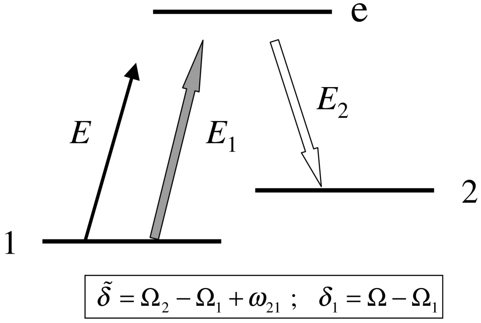
FIG. 1.: Schematic diagram of the atom-field system. Fields $E_{1}$ and $E$ drive only the $1-e$ transition and field $E_{2}$ only the $2-e$ transition.

The incident fields are assumed to be nearly copropagating so that all two-photon Doppler shifts can be neglected. In this limit and in the limit of large detuning on each single photon transition, one can consider the atoms to be stationary with regards to their interaction with the external fields. We wish to calculate the linear probe absorption spectrum. The electric field can be written as

$$E\left({\bf R,}t\right)=\frac{1}{2}\left[E_{1}e^{i\left({\bf k}_{1}\cdot{\bf R}-\Omega_{1}t\right)}+E_{2}e^{i\left({\bf k}_{2}\cdot{\bf R}-\Omega_{2}t\right)}\right.+\left.Ee^{i\left({\bf k}\cdot{\bf R}-\Omega t\right)}\right]+c.c.,$$ (1)

where $\Omega_{1},$ $\Omega_{2}$, and $\Omega$ are the field frequencies, ${\bf k}_{1},$ ${\bf k}_{2}$, and ${\bf k}$ the field propagation vectors, and $c.c.$ stands for complex conjugate. In an interaction representation, neglecting any decay or incoherent pumping of the ground state levels, the state probability amplitudes obey the equations of motion.

$$i\dot{a}_{e} = \chi_{1}e^{-i\Delta_{1}t}a_{1}+\chi_{2}e^{-i\Delta_{2}t}a_{2}+\chi e^{-i\Delta t}a_{1}$$ (4)

$$-i\left(\gamma_{e}/2\right)a_{e},$$

$$i\dot{a}_{1} = \chi_{1}e^{i\Delta_{1}t}a_{e}+\chi e^{i\Delta t}a_{e},$$ (5)

$$i\dot{a}_{2} = \chi_{2}e^{i\Delta_{2}t}a_{e},$$ (6)

where $\chi_{j}=-d_{ej}E_{j}/2\hbar$ ($j=1,2)$ and $\chi=-d_{e1}E/2\hbar$ are Rabi frequencies (assumed to be real and positive), $d_{ej}$ is a dipole moment matrix element, and $\Delta_{j}=\Omega_{j}-\omega_{ej}$ and $\Delta=\Omega-\omega_{e1}$ are atom-field detunings. Assuming that the magnitude of the detunings are much larger than $\gamma_{e}$ and any Doppler shifts associated with the single photon transitions, it is possible to adiabatically eliminate the excited state amplitude to arrive at the following equations for the ground state amplitudes:

$$i\dot{a}_{1} = S_{1}a_{1}+S\left(e^{i\delta_{1}t}+e^{-i\delta_{1}t}\right)a_{1}+ge^{-i\tilde{\delta}t}a_{2}$$ (9)

$$+g^{\prime}e^{-i\delta^{\prime}t}a_{2};$$

$$i\dot{a}_{2} = S_{2}a_{2}+ge^{i\tilde{\delta}t}a_{1}+g^{\prime}e^{i\delta^{\prime}t}a_{1},$$ (10)

where

$$\tilde{\delta} = \Delta_{2}-\Delta_{1}=\Omega_{2}-\Omega_{1}+\omega_{21};$$ (12)

$$\delta^{\prime} = \Delta_{2}-\Delta=\Omega_{2}-\Omega+\omega_{21};$$ (13)

$$\delta_{1} = \Delta-\Delta_{1}=\Omega-\Omega_{1}=\tilde{\delta}-\delta^{\prime},$$ (14)

are detunings associated with two-quantum processes and

$$g = \chi_{1}\chi_{2}/\Delta;\text{ \ }g^{\prime}=\chi\chi_{2}/\Delta;\text{ \ }$$ (15)

$$S_{1} = \chi_{1}^{2}/\Delta;\text{ \ }S_{2}=\chi_{2}^{2}/\Delta;\text{ \ }S=\chi\chi_{1}/\Delta,$$ (16)

are Rabi frequencies or Stark shifts associated with two quantum processes. In writing Eqs. (II), we assumed that $\Delta\approx\Delta_{1}\approx\Delta_{2}$ and $\left|\Delta\right|\gg\left|\tilde{\delta}\right|,\left|\delta^{\prime}\right|,\left|\delta_{1}\right|.$

It will prove convenient, especially when going over to a dressed atom picture, to introduce a representation in which

$$a_{1} = b_{1}e^{-i\tilde{\delta}t/2}e^{-i(S_{1}+S_{2})t/2};$$ (17)

$$a_{2} = b_{2}e^{i\tilde{\delta}t/2}e^{-i(S_{1}+S_{2})t/2}.$$ (18)

Combining Eqs. (II) and (18) one finds

$$i\dot{b}_{1} = -(\delta/2)b_{1}+gb_{2}+S\left(e^{i\delta_{1}t}+e^{-i\delta_{1}t}\right)b_{1}$$ (21)

$$+g^{\prime}e^{i\delta_{1}t}b_{2};$$

$$i\dot{b}_{2} = (\delta/2)b_{2}+gb_{1}+g^{\prime}e^{-i\delta_{1}t}b_{1},$$ (22)

where

$$\delta=\tilde{\delta}-(S_{1}-S_{2}).$$ (23)

The corresponding equations for density matrix elements $\rho_{11}=\left|b_{1}\right|^{2}$, $\rho_{22}=\left|b_{2}\right|^{2}$, $\rho_{12}=b_{1}b_{2}^{\ast}=\rho_{21}^{\ast}$ are

$$\dot{\rho}_{11} = -ig\left(\rho_{21}-\rho_{12}\right)-ig^{\prime}e^{i\delta_{1}t}\rho_{21}+ig^{\prime}e^{-i\delta_{1}t}\rho_{12}-\Gamma\rho_{11}+\Lambda_{1};$$ (25)

$$\dot{\rho}_{22} = ig\left(\rho_{21}-\rho_{12}\right)+ig^{\prime}e^{i\delta_{1}t}\rho_{21}-ig^{\prime}e^{-i\delta_{1}t}\rho_{12}-\Gamma\rho_{22}+\Lambda_{2};$$ (26)

$$\dot{\rho}_{12} = i\delta\rho_{12}-ig\left(\rho_{22}-\rho_{11}\right)-ig^{\prime}e^{i\delta_{1}t}\left(\rho_{22}-\rho_{11}\right)-iS\left(e^{i\delta_{1}t}+e^{-i\delta_{1}t}\right)\rho_{12}-\Gamma\rho_{12},$$ (27)

where the incoherent pumping and decay terms have been introduced. It is important to note that, in this representation, the frequency appearing in the $g^{\prime}$ terms is $\delta_{1}=\delta^{\prime}-\tilde{\delta}=\Omega-\Omega_{1}$. In other words, the effective field frequency associated with field $E_{2}$ in this representation is $\Omega_{1}$ rather than $\Omega_{2}$.

It follows from the Maxwell-Bloch equations that the probe absorption coefficient, $\alpha$, and index change, $\Delta n$, are given by

$$\alpha = \frac{kNd_{1e}^{2}}{2\hbar\epsilon_{0}}\mathop{\rm Im}\left(\frac{\rho_{1e}^{\prime}}{\chi}\right);$$ (29)

$$\Delta n = -\frac{Nd_{1e}^{2}}{2\hbar\epsilon_{0}}\mathop{\rm Re}\left(\frac{\rho_{1e}^{\prime}}{\chi}\right),$$ (30)

where $N$ is the atomic density,

$$\rho_{1e}^{\prime}\approx\frac{1}{\Delta}\left[\chi\rho_{11}^{(0)}+\chi_{1}\rho_{11}^{+}+\chi_{2}\rho_{12}^{+}\right],$$ (31)

and $\rho_{11}^{(0)}$, $\rho_{11}^{+}$, and $\rho_{12}^{+}$ are coefficients that appear in the solution of Eqs. (II) (to first order in $\chi$) written in the form:

$$\rho_{jj^{\prime}}=\rho_{jj^{\prime}}^{(0)}+\rho_{jj^{\prime}}^{+}e^{i\delta_{1}t}+\rho_{jj^{\prime}}^{-}e^{-i\delta_{1}t};\text{ \ \ \ }j,j^{\prime}=1,2$$ (32)

The first and third terms in Eq. (31) are analogous to the terms that appear in conventional theories of pump-probe spectroscopy, but the second term is new and leads to qualitatively new features in the probe absorption spectrum.

An expression for $\rho_{1e}^{\prime}$ is given in Appendix A. The absorption coefficient is plotted in Figs. 2(a)-(c) for several values of $\delta/g$, and

$$\eta=\sqrt{\chi_{1}/\chi_{2}}.$$ (33)

If $\eta\ll 1$, the two-quantum probe absorption spectrum has the same structure as the probe absorption spectrum involving single quantum transitions. The situation changes if $\eta\gtrsim 1$. For example, aside from an interchange of absorption and gain components as a function of $\delta$, the probe spectrum for single quantum transitions depends only on the magnitude of the pump field detuning. This is clearly not the case for two-quantum transitions, as is evident from Fig. 2(a) drawn for $\eta=1,$ $\Gamma/g=0.1$, $\delta/g=\pm 1$. Probe absorption and gain are interchanged when $\delta$ changes sign, but the ratio of the amplitude of the absorption to gain peak changes when $\delta$ changes sign. There is another subtle difference present in these spectra. The sense of the central dispersive component is opposite to that for single quantum transitions. With decreasing $\eta$ , the sense of the central component would reverse, as the spectrum reverts to the same structure found in pump-probe spectroscopy of single quantum transitions. The probe response also depends on the sign of $\Delta$ (through $g=\chi_{1}\chi_{2}/\Delta$); this feature follows from the dependence of the spectrum on the sign of $\delta$ and the relationship

$$\rho_{1e}^{\prime}(-\delta,-\Delta,-\delta_{1})=-\rho_{1e}^{\prime}(\delta,\Delta,\delta_{1})^{\ast},$$ (34)

which can be derived using Eqs. (A10)-(A) of Appendix A. It is also possible for the components centered at positive or negative $\delta_{1}$ to vanish (in the secular approximation) for certain values of $\eta$, as can be seen in Fig. 2(b).

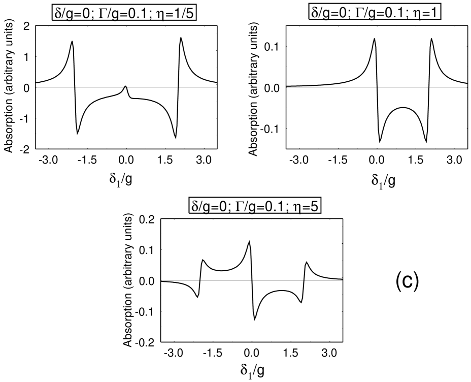
FIG. 2.: Probe field absorption in arbitrary units. Positive ordinate values correspond to probe absorption and negative values to probe gain.

The case of $\delta/g=0$ is shown in Fig. 2(c) for $\eta=1/5,1,$5, and $\Delta>0.$ If $\eta=1/5$, the spectrum is similar to that found for single quantum transitions [1]. For $\eta=1,$ the spectral component at negative $\delta_{1}$ is found to vanish. When $\eta\gtrsim 1$, there is a dispersive-like structure centered at $\delta_{1}=0$ that is not found in the pump-probe spectroscopy of single quantum transitions. Expressions for the three components are given in Eqs. (A8) of Appendix A for $\left|g\right|\gg\Gamma$, $\Gamma\ll\eta^{2}$.

III Dressed atom approach

The spectral features seen in Figs. 2 (a),(b) can be explained using a dressed atom approach. Semiclassical dressed states for two-quantum transitions can be introduced via the transformation [16]

$$\left(\begin{array}[]{c}\left|A\right\rangle\\ \left|B\right\rangle\end{array}\right) = {\bf T}\left(\begin{array}[]{c}\left|1\right\rangle\\ \left|2\right\rangle\end{array}\right);$$ (40)

$${\bf T} = \left(\begin{array}[]{cc}\cos\left(\theta\right)&-\psi\sin\left(\theta\right)\\ \psi\sin\left(\theta\right)&\cos\left(\theta\right)\end{array}\right),$$ (43)

where

$$\omega_{BA}=\sqrt{\delta^{2}+4g^{2}}$$ (44)

is the frequency separation of the dressed states,

$$\cos\left(\theta\right)=\left[\frac{1}{2}\left(1+\frac{\delta}{\omega_{BA}}\right)\right]^{1/2},$$ (45)

and

$$\psi=\left|\Delta\right|/\Delta.$$ (46)

The angle $\theta$ is restricted such that $0\leq\theta\leq\pi/4$ for $\delta>0$ and $\pi/4\leq\theta\leq\pi/2$ for $\delta<0$. For $\theta\sim 0$ ($\delta>0$, $\left|g/\delta\right|\ll 1$), $\left|A\right\rangle\sim\left|1\right\rangle$, while for $\theta\sim\pi/2$ $(\delta<0,$ $\left|g/\delta\right|\ll 1),$ $\left|B\right\rangle\sim\left|1\right\rangle$. In the secular approximation,

$$\Gamma\ll\omega_{BA},$$ (47)

it follows from Eqs. (II) and (III) that, to zeroth order in the probe field, the diagonal dressed state density matrix elements are given by

$$\left.\rho_{AA}^{(0)}=(\Lambda_{1}/\Gamma)\cos^{2}(\theta)+(\Lambda_{2}/\Gamma)\sin^{2}(\theta)\equiv\Lambda_{A}/\Gamma;\right.$$ (49)

$$\left.\rho_{BB}^{(0)}=(\Lambda_{2}/\Gamma)\cos^{2}(\theta)+(\Lambda_{1}/\Gamma)\sin^{2}(\theta)\equiv\Lambda_{B}/\Gamma;\right.$$ (50)

$$\left.\rho_{AA}^{(0)}-\rho_{BB}^{(0)}=\left(\Lambda_{A}-\Lambda_{B}\right)/\Gamma\right.$$ (51)

$$\left.=\left[(\Lambda_{1}-\Lambda_{2})/\Gamma\right]\cos(2\theta);.\right.$$ (52)

Note that $\left(\rho_{AA}^{(0)}-\rho_{BB}^{(0)}\right)$ has the same sign as $(\Lambda_{1}-\Lambda_{2})$ if $\delta>0$ and the opposite sign if $\delta<0.$

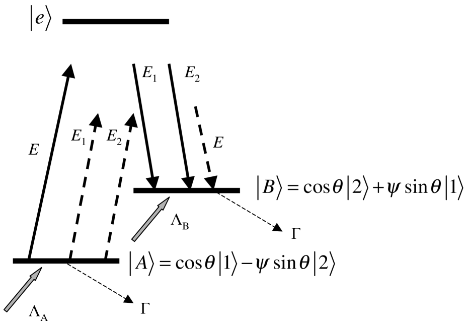
FIG. 3.: Dressed-state energy level diagram. In the interaction representation adopted in the text, the frequency of field $E_{2}$ must be set equal to $\Omega_{1}$ in calculating resonance conditions. For $\left(\Lambda_{A}-\Lambda_{B}\right)>0$, solid arrows correspond to probe absorption centered at $\delta_{1}=\omega_{BA}$ and dashed arrows correspond to probe gain centered at $\delta_{1}=-\omega_{BA}$.

It is now possible to use the energy level diagram (Fig. 3) to read directly the probe absorption spectrum. The probe field is absorbed (or amplified) via two quantum transitions between states $\left|A\right\rangle$ and $\left|B\right\rangle$. The two quantum transitions involve one photon from the probe field and one photon from either field $E_{1}$ or $E_{2}$, since all of these fields couple states $\left|A\right\rangle$ and $\left|B\right\rangle$ to state $\left|e\right\rangle$. It is important to remember that the effective field frequency of field $E_{2}$ is equal to $\Omega_{1}$ in this interaction representation. Fields $E_{1}$ and $E$ couple state $\left|e\right\rangle$ to the components of states $\left|A\right\rangle$ and $\left|B\right\rangle$ involving state $\left|1\right\rangle$, while field $E_{2}$ couples state $\left|e\right\rangle$ to the components of states $\left|A\right\rangle$ and $\left|B\right\rangle$ involving state $\left|2\right\rangle$. For example the matrix element for the two-quantum process from state $\left|A\right\rangle$ to $\left|B\right\rangle$ involving absorption of a probe photon and emission of a field $E_{2}$ photon is

$\displaystyle\frac{-i\chi}{-i\Delta}\cos(\theta)\frac{(-i\chi_{2})}{\Gamma-i(\delta_{1}-\omega_{BA})}\cos(\theta),$

while that for absorption of a probe photon and emission of a field $E_{1}$ photon is

$\displaystyle\frac{-i\chi}{-i\Delta}\cos(\theta)\frac{(-i\chi_{1})}{\Gamma-i(\delta_{1}-\omega_{BA})}\psi\sin(\theta).$

These two processes add coherently, such that probe absorption via transitions from state $\left|A\right\rangle$ to $\left|B\right\rangle$ is proportional to the sum of these two matrix elements squared, multiplied by the population difference $\left(\rho_{AA}^{(0)}-\rho_{BB}^{(0)}\right).$ In other words, the probe absorption at $\delta_{1}=\omega_{BA}$ is proportional to a quantity $C_{+}$ given by

$$C_{+}=\left(g/\Delta\Gamma\right)\left[(\Lambda_{1}-\Lambda_{2})/\Gamma\right]\cos\left(2\theta\right)\left(\psi\eta\sin\left(\theta\right)\cos(\theta)+\frac{1}{\eta}\cos^{2}\left(\theta\right)\right)^{2}.$$ (53)

Similarly, probe gain via transitions from state $\left|A\right\rangle$ to $\left|B\right\rangle$ at $\delta_{1}=-\omega_{BA}$ is proportional to

$$C_{-}=\left(g/\Delta\Gamma\right)\left[(\Lambda_{1}-\Lambda_{2})/\Gamma\right]\cos\left(2\theta\right))\left(\psi\eta\sin\left(\theta\right)\cos\left(\theta\right)-\frac{1}{\eta}\sin^{2}\left(\theta\right)\right)^{2}.$$ (54)

A formal derivation of these results is given in Appendix B.

For the sake of definiteness, let us take $(\Lambda_{1}-\Lambda_{2})>0;$ then $C_{+}$ corresponds to absorption for $\delta>0$ and to gain for $\delta<0$, while $C_{-}$ corresponds to gain for $\delta>0$ and to absorption for $\delta<0$. Note that the component centered at $\delta_{1}=-\omega_{BA}$ vanishes if $\Delta>0$ and $\tan(\theta)=\eta^{2}$, while that at $\delta_{1}=\omega_{BA}$ vanishes if $\Delta<0$ and $\tan(\theta)=\eta^{-2}$. The values of $A_{\pm}=\pm C_{\pm}\left[\Gamma^{2}\Delta/\left|g\right|(\Lambda_{1}-\Lambda_{2})\right]$ are plotted in Fig. 4 as a function of $\delta/g$ for $\Delta>0$ and $\eta=1,2$. For $\Delta<0$, one can use the relationship $A_{\pm}(-\Delta,-\delta)=A_{\mp}(\Delta,\delta)$.

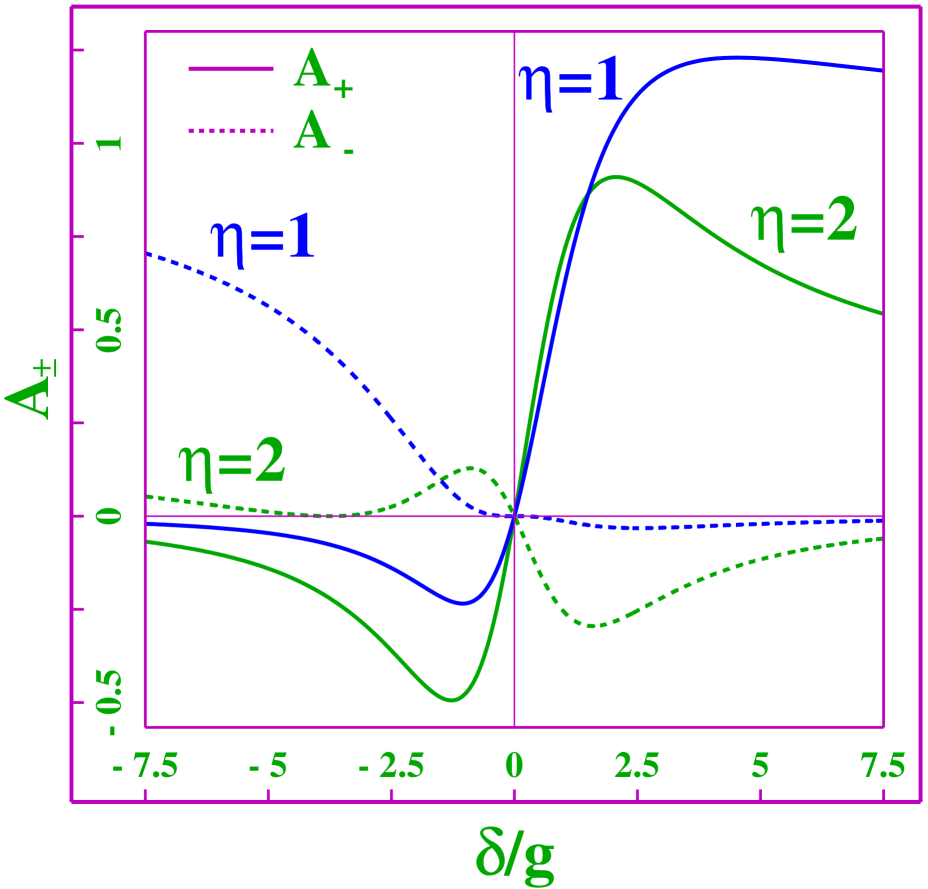
FIG. 4.: Amplitude $A_{+}$ of the peak centered at $\delta_{1}=\omega_{BA}$ and amplitude $A_{-}$ of the peak centered at $\delta_{1}=-\omega_{BA}$, for $\Delta>0.$ Positive values of $A_{\pm}$ correspond to absorption and negative values to gain.

The probe absorption vanishes in the secular approximation (47) when $\delta=0,$ since, in this case, $\theta=\frac{\pi}{4}$ and the populations of the dressed states are equal. The lowest order dressed atom approach is not useful in this limit. Typical spectra are shown in Fig. 2(c) and were discussed in Sec. III.

IV Conclusion

The probe absorption spectrum has been calculated for two-quantum transitions between levels that are simultaneously driven by a two-quantum pump field of arbitrary intensity. In addition to features found in conventional pump-probe spectroscopy of single quantum transitions, new features have been found that can be identified with interference phenomena. Both Doppler and recoil effects were neglected in out treatment. For nearly copropagating fields, effects arising from these processes are negligible. Doppler shifts can be accounted for by the replacements $\delta_{1}\rightarrow\delta_{1}+({\bf k}_{1}-{\bf k})\cdot{\bf v}$, $\delta_{1}-\tilde{\delta}\rightarrow\delta_{1}-\tilde{\delta}+({\bf k}_{2}-{\bf k})\cdot{\bf v,}$ and $\delta_{1}+\tilde{\delta}\rightarrow\delta_{1}+\tilde{\delta}+(2{\bf k}_{1}-{\bf k}_{2}-{\bf k})\cdot{\bf v}$ in the equations in the Appendix.

The dependence of the interference effect of the signs of $\Delta$ and $\tilde{\delta}$ can be understood in the bare atom picture in a perturbative limit. A schematic representation of the probability amplitude leading to probe absorption at $\delta_{1}=\tilde{\delta}$ is shown in Fig. 5(a). Each arrow represents an interaction with one of the fields. The two contributions to the final state amplitude add coherently. Putting in the appropriate energy denominators, one finds that the absorption varies as

$$A=\left|\frac{i^{2}\chi\chi_{2}^{\ast}}{\left(\gamma_{e}/2-i\Delta\right)\left[\Gamma-i\left(\Delta-\Delta_{2}\right)\right]}+\frac{i^{4}\chi\chi_{2}^{\ast}\left|\chi_{1}\right|^{2}}{\left(\gamma_{e}/2-i\Delta\right)\left[\Gamma-i\left(\Delta-\Delta_{1}\right)\right]\left(\gamma_{e}/2-i\Delta\right)\left[\Gamma-i\left(\Delta-\Delta_{2}\right)\right]}\right|^{2}.$$ (55)

For $\left|\tilde{\delta}\right|\gg\Gamma,$ and $\left|\Delta\right|\gg\gamma_{e}$, this equation reduces to

$$A=\left|\frac{\chi\chi_{2}^{\ast}}{\Delta}\right|^{2}\frac{1}{\Gamma^{2}+\left(\delta_{1}-\tilde{\delta}\right)^{2}}\left|1+\frac{\left|g\right|\eta^{2}\psi}{\tilde{\delta}}\right|,$$ (56)

which shows the dependence on the signs of $\Delta$ ($\psi=\left|\Delta\right|/\Delta)$ and $\tilde{\delta}.$ A similar calculation for the emission component represented schematically in Fig. 5(b) leads to

$$G=\left|\frac{\chi^{\ast}\chi_{1}^{2}\chi_{2}^{\ast}}{\Delta^{2}\tilde{\delta}}\right|^{2}\frac{1}{\Gamma^{2}+\left(\delta_{1}+\tilde{\delta}\right)^{2}}\left|1-\frac{\left|g\right|\eta^{-2}\psi}{\tilde{\delta}}\right|.$$ (57)

New effects will arise if the fields are not copropagating and the active medium is a subrecoil cooled atomic

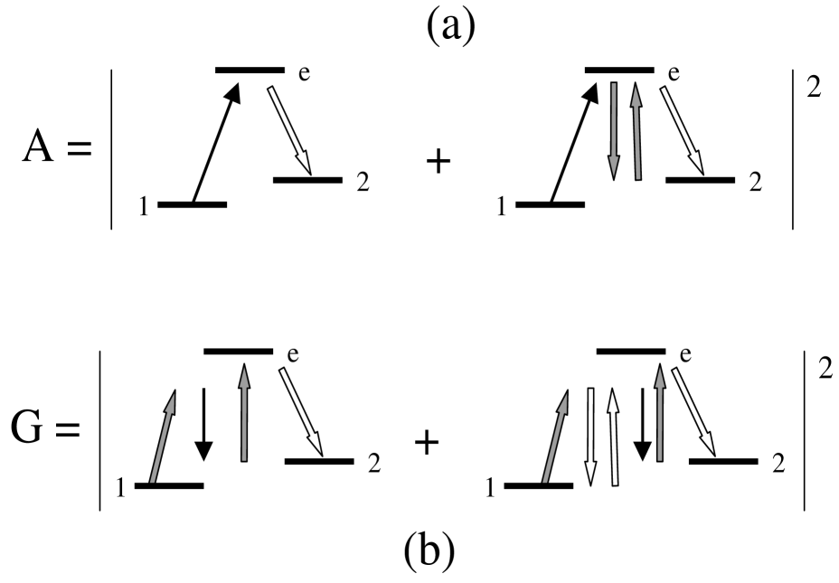
FIG. 5.: Schematic representation of the 1$\rightarrow 2$ transition probability leading to probe absorption or probe gain in lowest order perturbation theory in the bare basis. The thin arrow represents the probe field, the broad filled arrows field $E_{1}$, and the broad open arrows field $E_{2}$. (a) absorption, (b) gain. Terms involving the sequential absorption and emission of the same field have been neglected, since such terms result only in Stark shifts of levels $1$ and $2$. The diagrams are drawn for $\tilde{\delta}>0$; if $\tilde{\delta}<0$, the roles of absorption and gain would be interchanged.

vapor, a highly collimated atomic beam, or a BEC. As for single quantum transitions [7], each component of the spectrum undergoes recoil splitting. Since the center-of-mass momentum states differ for two-quantum processes involving fields $E_{1}$ and $E$ from those involving fields $E_{2}$ and $E$, one might expect the spectrum consists of eight absorption and eight emission components rather then the four absorption and four emission components found for single quantum transitions; however this does not appear to be the case. Instead, each component results from a coherent superposition of two quantum processes involving fields $\left(E_{1},E\right)$ and $\left(E_{2},E\right)$.

V Acknowledgments

This work is supported by the U. S. Army Research Office under Grant No. DAAG55-97-0113 and by the National Science Foundation under Grant No. PHY-9800981. We are grateful to the Prof. G. Raithel for fruitful discussions.

$\_\_\_\_\_\_\_\_\_\_\_\_\_\_\_\_\_\_\_\_\_\_\_\_\_\_\_\_\_\_\_\_\_\_\_\_\_\_\_\_\_\_\_\_\_\_\_\_\_\_\_\_\_\_\_\_\_\_\_\_\_\_\_\_\_\_\_\_\_\_\_\_\_\_\_\_\_\_\_\_\_\_\_\_\_\_\_\_\_\_\_\_\_\_\_\_\_\_\_\_\_\_\_\_\_\_\_\_\_\_\_\_\_\_\_\_\_\_\_\_\_\_\_\_\_\_\_\_\_\_\_\_\_\_\_\_$

A Bare State Calculations

Substituting Eqs. (32) into Eqs. (II), one finds to zeroth order in the probe field that

$$w^{(0)} = \rho_{22}^{(0)}-\rho_{11}^{(0)}=\frac{(\Lambda_{2}-\Lambda_{1})}{\Gamma}\frac{\Gamma^{2}+\delta^{2}}{\Gamma^{2}+\delta^{2}+4\left|g\right|^{2}};$$ (A2)

$$\rho_{11}^{(0)} = \frac{1}{2}\left[\frac{(\Lambda_{2}+\Lambda_{1})}{\Gamma}-w^{(0)}\right];$$ (A3)

$$\rho_{12}^{(0)} = \frac{-ig}{\Gamma-i\delta}w^{(0)}=\left(\rho_{21}^{(0)}\right)^{\ast},$$ (A4)

and that, to first order in the probe field, $w^{+}=\rho_{22}^{+}-\rho_{11}^{+}$, $\rho_{12}^{+}$, $\rho_{21}^{+}$, and $m^{+}=\rho_{22}^{+}+\rho_{11}^{+}$ satisfy

$$\left.m^{+}=0;\right.$$ (A6)

$$\left.\left(\Gamma+i\delta_{1}\right)w^{+}-2ig^{\ast}\rho_{21}^{+}+2ig\rho_{12}^{+}=2ig^{\prime}\rho_{21}^{(0)};\right.$$ (A7)

$$\left.\left[\Gamma+i\left(\delta_{1}-\delta\right)\right]\rho_{12}^{+}+ig^{\ast}w^{+}=-ig^{\prime\ast}w^{(0)}-iS\rho_{12}^{(0)};\right.$$ (A8)

$$\left.\left[\Gamma+i\left(\delta_{1}+\delta\right)\right]\rho_{21}^{+}-igw^{+}=iS\rho_{21}^{(0)}.\right.$$ (A9)

Equation (31) can be rewritten as

$$\rho_{1e}^{\prime}\approx(\chi^{\ast}/\Delta)\left[\rho_{11}^{(0)}-\frac{1}{2}y_{0}+y_{12}\right],$$ (A10)

where

$$y_{0} = \left(\chi_{1}/\chi\right)^{\ast}w^{+};$$ (A12)

$$y_{12} = \left(\chi_{2}/\chi\right)^{\ast}\rho_{12}^{+};$$ (A13)

$$y_{21} = \left(\frac{\chi_{2}\chi_{{}_{1}}^{\ast}}{\chi^{\ast}\chi_{1}}\right)\rho_{21}^{+}.$$ (A14)

In Eqs. (A-A10) we have allowed the Rabi frequencies to be complex.

The quantities $y_{0}$, $y_{12}$, and $y_{21}$ satisfy the coupled equations:

$$\left[\Gamma+i\left(\delta_{1}-\delta\right)\right]y_{12}+i\left|g\right|\psi\eta^{-2}y_{0} = a;$$ (A16)

$$\left(\Gamma+i\delta_{1}\right)y_{0}-2i\left|g\right|\psi\eta^{2}y_{21}+2i\left|g\right|\psi\eta^{2}y_{12} = b;$$ (A17)

$$\left[\Gamma+i\left(\delta_{1}+\delta\right)\right]y_{21}-i\left|g\right|\psi\eta^{-2}y_{0} = c,$$ (A18)

where

$$b = \frac{-2\left|g\right|^{2}}{\Gamma+i\delta}w^{(0)}=2c$$ (A20)

$$a = -i\left|g\right|\psi\eta^{-2}w^{(0)}-\frac{\left|g\right|^{2}}{\Gamma-i\delta}w^{(0)}.$$ (A21)

and $\psi=(\left|\Delta\right|/\Delta)$. Note that the equations do not depend on the phase of the various Rabi frequencies, but do depend on the sign of $\Delta$. Explicit solutions for $y_{0}$ and $y_{12}$ are:

$$y_{0} = -i\frac{2a\left|g\right|\psi\eta^{2}\left(\delta+\delta_{1}-i\Gamma\right)+b\left[\delta^{2}-\left(\delta_{1}-i\Gamma\right)^{2}\right]+2c\left|g\right|\psi\eta^{2}\left(\delta-\delta_{1}+i\Gamma\right)}{\left(\delta_{1}-i\Gamma\right)\left(\delta^{2}-\delta_{1}^{2}+2i\Gamma\delta_{1}+\Gamma^{2}+4\left|g\right|^{2}\right)};$$ (A23)

$$y_{12} = i\frac{a\left[\delta_{1}^{2}+\delta\left(\delta_{1}-i\Gamma\right)-2i\Gamma\delta_{1}-\Gamma^{2}-2\left|g\right|^{2}\right]-b\eta^{-2}\left|g\right|\psi\left(\delta+\delta_{1}-i\Gamma\right)-2c\left|g\right|^{2}}{\left(\delta_{1}-i\Gamma\right)\left(\delta^{2}-\delta_{1}^{2}+2i\Gamma\delta_{1}+\Gamma^{2}+4\left|g\right|^{2}\right)}.$$ (A24)

The line shape is totally non-secular when $\delta=0.$ In the limit that $\Delta>0$, $\left|g\right|\gg\Gamma$, and $\Gamma\ll\eta^{2},$ one finds that the absorption coefficient $\alpha$ for $\delta_{1}\approx 0$ is

$$\alpha\sim-\frac{1}{4}\left(\frac{kNd_{1e}^{2}}{2\hbar\epsilon_{0}\Delta}\right)\frac{\Lambda_{1}-\Lambda_{2}}{\Gamma}\frac{\delta_{1}\Gamma}{\left(\delta_{1}^{2}+\Gamma^{2}\right)},$$ (A25)

that for $\delta_{1}\approx 2\left|g\right|$ is

$$\alpha\sim\frac{1}{8}\left(\frac{kNd_{1e}^{2}}{2\hbar\epsilon_{0}\Delta}\right)\frac{\Lambda_{1}-\Lambda_{2}}{\Gamma}\frac{\left(\delta_{1}-2\left|g\right|\right)\Gamma}{\left[\left(\delta_{1}-2\left|g\right|\right)^{2}+\Gamma^{2}\right]}(1+\eta^{-2}),$$ (A25)

and that for $\delta_{1}\approx-2\left|g\right|$ is

$$\alpha\sim\frac{1}{8}\left(\frac{kNd_{1e}^{2}}{2\hbar\epsilon_{0}\Delta}\right)\frac{\Lambda_{1}-\Lambda_{2}}{\Gamma}\frac{\left(\delta_{1}+2\left|g\right|\right)\Gamma}{\left[\left(\delta_{1}+2\left|g\right|\right)^{2}+\Gamma^{2}\right]}(1-\eta^{-2}).$$ (A26)

Note that the component at $\delta_{1}=-2\left|g\right|$ vanishes if $\eta=1$. For $\Delta<0$, one can use Eq. (34).

B Dressed-State Calculations

Equation (II) can be written in the form

$$i\hbar{\bf\dot{b}}=\left({\bf V+V}_{p}\right){\bf b},$$ (B1)

where

$${\bf V}=\hbar\left(\begin{array}[]{cc}-\delta/2&g^{\ast}\\ g&\delta/2\end{array}\right),$$ (B2)

$${\bf V}_{p}=\hbar\left(\begin{array}[]{cc}Se^{i\delta_{1}t}+S^{\ast}e^{-i\delta_{1}t}&g^{\prime\ast}e^{i\delta_{1}t}\\ g^{\prime}e^{-i\delta_{1}t}&0\end{array}\right),$$ (B3)

$$g=\frac{\chi_{1}\chi_{2}^{\ast}}{\Delta};\text{ \ }g^{\prime}=\frac{\chi\chi_{2}^{\ast}}{\Delta};\text{ \ }S=\frac{\chi^{\ast}\chi_{1}}{\Delta},$$ (B4)

and we have allowed for complex Rabi frequencies,

$$\chi_{1}=\left|\chi_{1}\right|e^{i\phi_{1}},\chi_{2}=\left|\chi_{2}\right|e^{i\phi_{2}},\chi=\left|\chi\right|e^{i\phi}.$$ (B5)

If one introduces semi-classical dressed states via the transformation

$${\bf b}_{d}={\bf T}_{c}{\bf b},$$ (B6)

where

$${\bf b}_{d}=\left(\begin{array}[]{c}A\\ B\end{array}\right),$$ (B7)

$${\bf T}_{c}=\left(\begin{array}[]{cc}\cos\left(\theta\right)e^{i\phi_{d}/2}&-e^{-i\phi_{d}/2}\sin\left(\theta\right)\\ e^{i\phi_{d}/2}\sin\left(\theta\right)&e^{-i\phi_{d}/2}\cos\left(\theta\right)\end{array}\right),$$ (B8)

and

$$\phi_{d}=\phi_{1}-\phi_{2}+\frac{\pi}{2}(1-\psi)$$ (B9)

(recall that $\psi=\left|\Delta\right|/\Delta$), then the dressed-state Hamiltonian is given by

$${\bf V}_{d}=\hbar\left(\begin{array}[]{cc}-\omega_{BA}/2&0\\ 0&\omega_{BA}/2\end{array}\right)+{\bf T}_{c}{\bf V}_{p}{\bf T}_{c}^{{\bf\dagger}}.$$ (B10)

The dressed state density matrix,

$${\bf\rho}_{d}=\left(\begin{array}[]{cc}\rho_{AA}&\rho_{AB}\\ \rho_{BA}&\rho_{BB}\end{array}\right)$$ (B11)

evolves as

$$\left(\frac{d}{dt}+\Gamma\right){\bf\rho}_{d}\approx\frac{1}{i\hbar}\left[{\bf V}_{d},{\bf\rho}_{d}\right]+\left(\begin{array}[]{cc}\Lambda_{A}&0\\ 0&\Lambda_{B}\end{array}\right),$$ (B12)

Off-diagonal terms have been neglected in the matrix representing the incoherent pumping, since they give rise to terms of order $\Gamma/\omega_{BA}\ll 1$ (secular approximation).

The dressed state density matrix is expanded as

$${\bf\rho}_{d}={\bf\rho}_{d}^{(0)}+{\bf\rho}_{d}^{+}e^{i\delta_{1}t}+{\bf\rho}_{d}^{-}e^{-i\delta_{1}t},$$ (B13)

and it is found from Eqs. (B1)-(B3), (B6)-(B13) that ${\bf\rho}_{d}^{+}$ obeys the equation of motion

$$\left(\frac{d}{dt}+\Gamma\right){\bf\rho}_{d}^{+}=i\left(\begin{array}[]{cc}0&\left(\omega_{BA}-\delta_{1}\right)\rho_{AB}^{+}\\ -\left(\omega_{BA}+\delta_{1}\right)\rho_{BA}^{+}&0\end{array}\right)+\frac{1}{i\hbar}\left[{\bf V}_{pd},{\bf\rho}_{d}^{(0)}\right],$$ (B14)

where

$${\bf V}_{pd}=\hbar\left(\begin{array}[]{cc}\cos\left(\theta\right)\left[S\cos\left(\theta\right)-g^{\prime\ast}e^{i\phi_{d}}\sin\left(\theta\right)\right];&\cos\left(\theta\right)\left[S\sin\left(\theta\right)+g^{\prime\ast}\cos\left(\theta\right)e^{i\phi_{d}}\right]\\ \sin\left(\theta\right)\left[-g^{\prime\ast}\sin\left(\theta\right)e^{i\phi_{d}}+S\cos\left(\theta\right)\right];&\sin\left(\theta\right)\left[S\sin\left(\theta\right)+g^{\prime\ast}\cos\left(\theta\right)e^{i\phi_{d}}\right]\end{array}\right)$$ (B15)

In the secular approximation, the steady state solution of Eq. (B14) is

$${\bf\rho}_{d}^{+}=\left(\begin{array}[]{cc}0&\rho_{AB}^{+}\\ \rho_{BA}^{+}&0\end{array}\right),$$ (B16)

where

$$\rho_{AB}^{+} = i\cos\left(\theta\right)\left[S\sin\left(\theta\right)+g^{\prime\ast}\cos\left(\theta\right)e^{i\phi_{d}}\right]\left(\rho_{AA}^{(0)}-\rho_{BB}^{(0)}\right)/\left(\Gamma+i\left(\delta_{1}-\omega_{BA}\right)\right),$$ (B18)

$$\rho_{BA}^{+} = -i\sin\left(\theta\right)\left[-g^{\prime\ast}\sin\left(\theta\right)e^{i\phi_{d}}+S\cos\left(\theta\right)\right]\left(\rho_{AA}^{(0)}-\rho_{BB}^{(0)}\right)/\left(\Gamma+i\left(\delta_{1}+\omega_{BA}\right)\right).$$ (B19)

The coherence $\rho_{1e}^{\prime}$ needed in Eq. (1) for the absorption coefficient and index change is given by

$$\rho_{1e}^{\prime}\approx(1/\Delta)\left[\chi^{\ast}\rho_{11}^{(0)}+\chi_{1}^{\ast}\rho_{11}^{+}+\chi_{2}^{\ast}\rho_{12}^{+}\right].$$ (B20)

The first term can be evaluated using Eq. (A3) for $\rho_{11}^{(0)}$; it contributes to the index change, but not the absorption. For the remaining terms, one rewrites $\rho_{11}^{+}$ and $\rho_{12}^{+}$ in the dressed basis using Eqs. (B6),(B8),(B11), and uses Eq. (B5) to extract all the phase factors to arrive at

$$\rho_{1e}^{\prime}\approx(\chi^{\ast}/\left|\Delta\right|)\left[\psi\rho_{11}^{(0)}+f_{+}+f_{-}\right]$$ (B21)

where

$$f_{+} = \frac{i\left|g\right|}{\left[\Gamma+i\left(\delta_{1}-\omega_{BA}\right)\right]}\cos\left(2\theta\right)\frac{\left(\Lambda_{1}-\Lambda_{2}\right)}{\Gamma}\cos^{2}(\theta)\left(\psi\eta\sin\left(\theta\right)+\frac{1}{\eta}\cos\left(\theta\right)\right)^{2},$$ (B23)

$$f_{-} = -\frac{i\left|g\right|}{\left[\Gamma+i\left(\delta_{1}+\omega_{BA}\right)\right]}\cos\left(2\theta\right)\frac{\left(\Lambda_{1}-\Lambda_{2}\right)}{\Gamma}\sin^{2}(\theta)\left(\psi\eta\cos\left(\theta\right)-\frac{1}{\eta}\sin\left(\theta\right)\right)^{2}.$$ (B24)

Note that the approach and results of Sec. III are unchanged if one uses complex dressed states defined by

$$\left(\begin{array}[]{c}\left|A\right\rangle\\ \left|B\right\rangle\end{array}\right)={\bf T}_{c}^{\ast}\left(\begin{array}[]{c}\left|1\right\rangle\\ \left|2\right\rangle\end{array}\right).$$ (B25)

REFERENCES

• [1] B. R. Mollow, Phys. Rev. A 5, 2217 (1972).
• [2] S. Haroche and S. Hartmann, Phys. Rev. A 6, 1280 (1972).
• [3] F. Y. Wu, S. Ezekiel, M. Ducloy, and B. R. Mollow, Phys. Rev. Lett. 38, 1077 (1977).
• [4] C. Cohen-Tanoudji and S. Reynaud, J. Phys. B 10, 345 (1977).
• [5] G. Grynberg and C. Cohen-Tannoudji, Optics Comm. 96, 150 (1993).
• [6] P. R. Berman and G. Khitrova, Optics Comm. xx, xxxx (2000).
• [7] P. R. Berman, B. Dubetsky, and J. Guo, Phys. Rev. A 51, 3947 (1995).
• [8] See, for example, P. D. Lett, W. D. Phillips, S. L. Rolston, C. E. Tanner, R. N. Watts, and C. I. Westbrook, J. Opt. Soc. Am. B 6, 2084 (1989); J. Dalibard and C. Cohen-Tannoudji, ibid. 6, 2023 (1989); P. J. Ungar, D. S. Weiss, E. Riis, and S. Chu, ibid. 6, 2058 (1989); D. S. Weiss, E. Riis, Y. Shevy, P. J. Ungar, and S. Chu, ibid. 6, 2072 (1989); A. Aspect, E. Arimondo, R. Kaiser, N. Vanteenkiste, and C. Cohen-Tannoudji, ibid. 6, 2112 (1989).
• [9] A. Aspect, E. Arimondo, R. Kaiser, N. Vansteenkiste, and C. Cohen-Tannoudji, Phys. Rev. Lett. 61, 826 (1988); M. Kasevich and S. Chu, Phys. Rev. Lett. 69, 1741 (1992).
• [10] M. Prentiss, G. Timp, N. Bigelow, R. E. Behringer, J. E. Cunningham, Appl. Phys. Lett. 60, 1027, (1992); T. Sleator, T. Pfau, V. Balykin, and J. Mlynek, Appl. Phys. B 54, 375 (1992).
• [11] Atom Interferometry, edited by P.R. Berman (Academic, San Diego, 1997).
• [12] D. S. Weiss, B. C. Young, S. Chu, Phys. Rev. Lett. 70, 2706 (1993).
• [13] A. Peters, K. Y. Chung, and S. Chu, Nature, 400, 849 (1999).
• [14] T. L. Gustavson, P. Bouyer, and M. A. Kasevich, Phys. Rev. Lett. 78, 2046 (1997).
• [15] D. M. Stamper-Kurn, A. P. Chikkatur, A. Görlitz, S. Innouye, S. Gupta, D. E. Pritchard, and W. Ketterle, Phys. Rev. Lett. 83, 2876 (1999).
• [16] P. R. Berman, Phys. Rev. A 53, 2627 (1996).
Conversion to HTML had a Fatal error and exited abruptly. This document may be truncated or damaged.