Measurement of Carbon Disulfide Anion Diffusion in a TPC

Abstract

A Negative Ion Time Projection Chamber was used to measure the field dependence of lateral and longitudinal diffusion for CS₂ anions drifting in mixtures of CS₂ and Ar at 40 Torr. Ion drift velocities and limits on the capture distance for electrons as a function of field and gas mixture are also reported.

,

1 Introduction

The Directional Recoil Identification From Tracks (DRIFT) detector has recently been proposed [1] to search for dark matter. This detector is unique in that it drifts negative ions, instead of electrons, in a time projection chamber (TPC). A detailed description of the operation, motivation, and other uses of a negative ion TPC (NITPC) can be found in [2]. Briefly, an electronegative component in the gas captures ionized electrons forming negative ions. These anions then drift to the anode wires where, provided the electronegative component allows it, the anions are ionized and normal electron avalanche occurs. The motivation for such an arrangement is that it allows transport of charge to the anode with the minimum possible diffusion. Using a proportional chamber, Crane showed that CS₂ has the desired electronegative properties [3]. Using a single wire drift chamber of unusual design, Martoff et al. [2] measured the drift velocity and lateral diffusion of CS₂ ions in two different gas mixtures. In this paper we used a NITPC to measure the drift velocity, lateral diffusion and longitudinal diffusion in a variety of CS₂-Ar gas mixtures. These measurements allowed limits to be set on the electron capture distance in these mixtures.

2 Theory

The diffusion of charged particles being drifted through a gas has been parameterized by an expression of the form [4]:

$$\sigma^{2}=\frac{4\varepsilon_{\mathrm{k}}L}{3eE}$$ (1)

where $L$ is the drift distance, $E$ is the drift field and $\varepsilon_{\mathrm{k}}$ is the characteristic (average) energy of the electron or ion. For electrons, $\varepsilon_{\mathrm{k}}$ varies from thermal ($\sim k_{\mathrm{B}}T$) at low drift fields to several eV at higher $E/p$. The nonlinear variation of $\varepsilon_{\mathrm{k}}$ for electrons arises from the mass mismatch between electrons and gas atoms which prevents elastic electron–atom collisions from efficiently thermalizing the electron energy gained between collisions [5]. Ions, on the other hand, have masses comparable to the gas atoms and hence would be expected to remain well thermalized even if the energy gained between collisions became comparable with $\sim k_{\mathrm{B}}T$. Thus $\varepsilon_{\mathrm{k}}$ for ions should remain constant and one should be able to reduce the diffusion of ions (as 1/$\sqrt{E}$) to much lower values than for electrons. The NITPC concept relies critically on this hypothesis. The purpose of the present work was to test it in detail.

3 Experimental Method

3.1 Apparatus

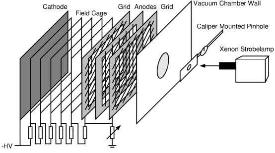
Figure 1: TPC in Situ (not to scale)

The NITPC used in this experiment consisted of a drift region attached to a multi-wire proportional chamber (MWPC) (Figure 1). The drift region was composed of a solid copper cathode and field cage. The field cage consisted of 4 loops of 500 $\mu$m wire supported by acrylic posts and connected by a ladder of precision 10 M$\Omega$ resistors. The lateral dimensions of the field cage were 15 cm by 20 cm. The MWPC was made of three wire planes: two grid planes sandwiching an anode plane. The grid and anode wires were 100 $\mu$m and 20 $\mu$m gold coated tungsten respectively. Anode wire spacing was 2 mm, grid wire spacing was also 2 mm but at 45 degrees to the anodes and the gap was 1.1 cm. The drift distance, from the solid copper cathode to the nearest grid plane, was 10 cm.

A single negative high voltage supply connected at the cathode was used to set the drift and MWPC potentials via the field cage resistance and a variable resistance between anode and grid. During operation, the MWPC voltage was kept as high as possible to yield the greatest gas gain and to insure 100% transparency [4].

The detector was mounted with wire planes vertical in an evacuable chamber. Gas mixtures were prepared in the chamber by introducing gases one by one through a manifold. CS₂ vapor was evolved from a liquid source by the low pressure in the chamber. All experiments were done at a pressure of 40.0 Torr. The chamber pressure was measured with a capacitive manometer allowing accurate (0.1 Torr) determination of pressure and mixture. Before each run, the chamber was evacuated to $\sim$ 50 mTorr measured using a Convectron gauge, then backfilled with the desired gas mixture and pressure. A gas filling would be used for several hours, during which time the pressure rise was about a percent.

The diffusion measurements were made using photoelectrons generated from the solid copper cathode in the following way. Near the NITPC was a port containing a fused silica window. A UV flashlamp projected light through a movable 200 $\mu$m aperture, through the silica window, through the grid and anode wire planes, and onto the cathode. The projected spot on the cathode was $\sim$ 1.3 mm by $\sim$ 2 mm measured using photographic film. To maintain the photoelectron yield, the copper cathode was cleaned with abrasive every three to five runs. A photodiode viewing the flashlamp directly provided a start signal for drift time measurements.

The anode wires were connected to Amptek A-250 charge sensitive pre-amplifiers which were housed inside the chamber to reduce noise pickup. The outputs of the Ampteks were amplified and shaped by Ortec 855 spectroscopy amplifiers. These signals were digitized and stored on a 20 MHz digital oscilloscope. The scope used the photodiode signal as a trigger. Waveform averaging was used to improve signal to noise.

3.2 Measurement

To measure the lateral diffusion, the maximum pulse heights on two adjacent wires were measured as the aperture was moved laterally through 40, 125 $\mu$m steps. Pulse height maxima were measured on waveforms averaged over either 128 or 256 individual flashlamp shots. Space charge should not affect the results of this experiment. The number of photoelectrons produced was always less than $\sim$ 50 per flash. The lateral diffusion of the anions was always greater than 0.7 mm. Since the gain was low, $\sim$ 3000, the size of the avalanche was $\sim$ 0.05 mm [4]. In those cases where two avalanches overlapped, the reduction in gain for the second avalanche was less than 1% [4]. In addition to these theoretical arguments, the gain linearity was tested by confirming that a $\times$10 reduction in flash energy resulted in an order of magnitude reduction in pulse height.

Figure 2: Two–Gaussian Fit to Typical Data Set

Figure 2 shows a set of measurements, with aperture position on the horizontal axis and pulse height of the averaged waveforms on the vertical axis. The data for each peak was fit to a function that allowed deconvolution of the deposited charge from a known electronic artifact. The distance between the two peaks represented the 2 mm wire spacing and was used to normalize the lateral measurement. The +’s and $\times$’s in Figure 2 are the data for each wire, the line is the fitted function.

The longitudinal diffusion was determined by measuring the pulse width in time on a single wire. To convert this measurement to distance, the drift speed as a function of drift field was determined for each gas mixture. This was done by measuring the delay time between the light pulse (photoelectron generation) and the peak of the anode signal. Though the majority of the delay was due to the time ions spent in the drift field, a correction was made for the delay in the MWPC.

In order to minimize variations due to changing chamber conditions, a set of runs at different drift fields would be done with a given gas mixture. Additionally, all of the above measurements (lateral and longitudinal diffusion and drift velocity) were done concurrently at a given drift field. The delay time and pulse time-width were both measured at the aperture position corresponding to maximum pulse height for the wire under test. To reduce the effects of gas aging, a gas mixture was kept for only one set of runs, and was flushed at the end of the day.

4 Results and Discussion

There are a number of contributions to the measured $\sigma$. The main ones are the finite spot size, geometry of the chamber, capture distance, and the diffusion itself(given by Equation 1). Since the gap distance in the MWPC was so small and the field so large the diffusion there was assumed to be minimal. The various contributions can be assumed to be uncorrelated and hence to add in quadrature:

$$\sigma_{\mathrm{measured}}^{2}=\sigma_{\mathrm{spot}}^{2}+\sigma_{\mathrm{geometry}}^{2}+\sigma_{\mathrm{capture}}^{2}+\frac{2k_{\mathrm{B}}T_{\mathrm{eff}}L}{e}\frac{1}{E}$$ (2)

where $\varepsilon_{\mathrm{k}}$ in Equation 1 has been characterized in terms of an effective temperature $T_{\mathrm{eff}}$. The NITPC hypothesis is that $T_{\mathrm{eff}}$ will remain constant and close to room temperature up to very high drift fields.

For the lateral measurements, the $\sigma_{\mathrm{spot}}$ was significant while for the longitudinal measurements it was not due to the short duration of the pulse. In the lateral measurements $\sigma_{\mathrm{geometry}}$ arises from the 2 mm wire spacing and is significant. For the longitudinal measurements $\sigma_{\mathrm{geometry}}$ arises from the different pathlengths ions can take to get to the anode wires and is also significant. None of these is a function of the field.

Since $\sigma_{\mathrm{capture}}$ is expected to increase with increasing field, a linear relationship between $\sigma_{\mathrm{measured}}^{2}$ and $1/E$ supports the assumption that $\sigma_{\mathrm{capture}}$ is slowly varying or constant. In that case, $T_{\mathrm{eff}}$ can be deduced from the slope. The capture distance can be deduced from the intercept if the geometry and spot size contributions are known or estimated, since according to Equation 2

$$\sigma_{\mathrm{capture}}^{2}=\sigma_{\mathrm{intercept}}^{2}-\sigma_{\mathrm{geometry}}^{2}-\sigma_{\mathrm{spot}}^{2}$$ (3)

4.1 Lateral Diffusion

The main lateral diffusion results are summarized in Figure 3 and Table 1. The plot shows the lateral diffusion squared ($\sigma^{2}$) versus the inverse of the drift field.

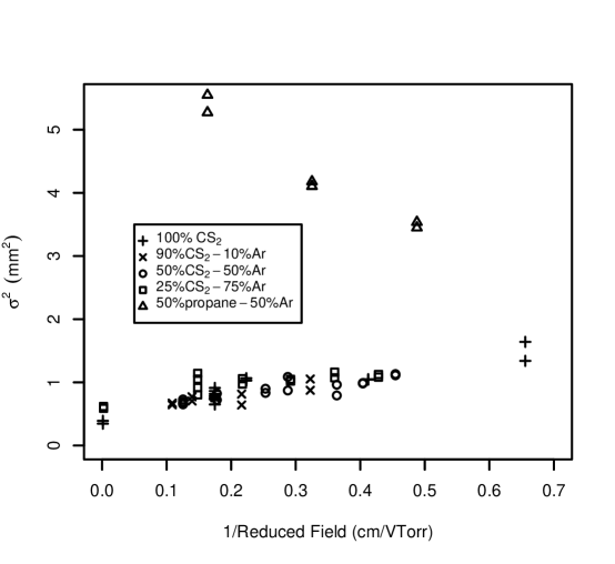
Figure 3: Lateral Diffusion for Various Gas Mixtures

Table 1: Lateral Diffusion Results

Gas Mixture Slope Temperature Y-Intercept $\sigma_{capture}$ 100%CS₂ 0.16 $\pm$0.02 Vmm/Torr 360 $\pm$40 K 0.50 $\pm$0.05 mm² $<$0.4 mm 90%CS₂-10%Ar 0.13 $\pm$0.03 Vmm/Torr 300 $\pm$80 K 0.52 $\pm$0.07 mm² $<$0.4 mm 50%CS₂-50%Ar 0.11 $\pm$0.02 Vmm/Torr 260 $\pm$40 K 0.56 $\pm$0.05 mm² $<$0.5 mm 25%CS₂-75%Ar 0.10 $\pm$0.02 Vmm/Torr 240 $\pm$50 K 0.74 $\pm$0.06 mm² $<$0.6 mm

On the graph, the marks represent the data taken for different gas mixtures at a variety of drift fields. The triangles are electrons drifted in 50% propane-50%argon for reference. The points very close to the origin are from experiments where the drift region was removed and the MWPC used alone with a copper cathode in place of one of the grid planes. The copper cathode was in approximately the same position relative to the light source for both the MWPC and NITPC measurements so that the spot size was constant. The reason that several diffusion values appear for each drift field is that two wires were used during the measurement. Since the uncertainty in the Gaussian fits for the points is much smaller than the marks, the separation between the points at identical fields represents a systematic error. This is believed to be due to the modulation of UV light intensity by the grid and anode wires.

Clearly, the electron data (open triangles in Figure 3) do not obey Equation (2), but all of the ion data do. The ion data were fit to lines from which $T_{\mathrm{eff}}$ and the intercept were extracted. As can be seen in Table 1, all of the temperatures are consistent with thermal diffusion with perhaps a hint that the lateral diffusion is decreasing with increasing concentration of Ar.

The fact that the high field points lie on the general trend of the data is important in that it shows that electrons are captured even in very large E/p. For the 100% CS₂ data the high field was 83 V/cmTorr while for the 25%  CS₂ - 75% Ar data it was 45 V/cmTorr. The intercept data shown in Table 1 and Equation 3 can now be used to figure out $\sigma_{\mathrm{capture}}$. Given the crude nature of our photographic measurement $\sigma_{\mathrm{spot}}$ could not be estimated with any reliability. However, $\sigma_{\mathrm{geometry}}=2mm/\sqrt{12}$ which allows to us to place the upper limits on $\sigma_{\mathrm{capture}}$ shown in Table 1.

4.2 Mobility

Figure 4 shows the drift velocity data for the gas mixtures plotted against the reduced field. The data from each of the gas mixtures was fitted to $v=m(E/p)+n(E/p)^{2}$.

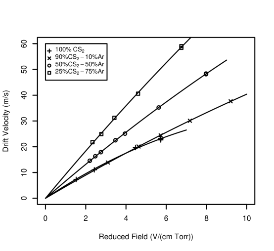
Figure 4: Drift Velocity vs. Field

Table 2: Mobility Coefficients

Gas Mixture m n 100%CS₂ 5.2 $\pm$0.2 -0.20 $\pm$0.03 90%CS₂-10%Ar 4.6 $\pm$0.03 -0.057 $\pm$0.004 50%CS₂-50%Ar 6.77 $\pm$0.03 -0.090 $\pm$0.005 25%CS₂-75%Ar 9.4 $\pm$0.1 -0.10 $\pm$0.02

Table 2 shows the drift velocity coefficients for the different gas mixtures. The drift velocity increases with increasing concentration of argon. This is not unexpected as an Ar atom is much smaller than a CS₂ molecule and therefore the mean free path of the CS₂ ions is much larger, the mean time to collision is increased, thus yielding a higher drift velocity. In addition the larger mass of the CS₂ molecule means that it will preferentially scatter off of the Ar atoms in the forward direction.

4.3 Longitudinal Diffusion

The longitudinal diffusion results are shown in Figure 5 and Table 3. As in the lateral case, the rms diffusion squared is plotted against the inverse of the reduced drift field.

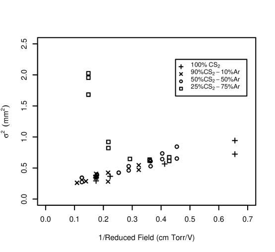
Figure 5: Longitudinal Diffusion

As before, the marks represent the data for the various gas mixtures. All of the data look linear with the obvious exception of the 25%CS₂-75%Ar mixture. The linear datasets were fit to straight lines, giving the $T_{\mathrm{eff}}$ values and intercepts shown in Table 3. Notice that in this case the trend is for the temperature to increase with increasing concentration of Ar.

Table 3: Longitudinal Diffusion Results

Gas Mixture Slope Temperature Y-Intercept $\sigma_{capture}$ 100%CS₂ 0.10 $\pm$0.01 Vmm/Torr 230 $\pm$20 K 0.17 $\pm$0.02 mm² $<$0.4 mm 90%CS₂-10%Ar 0.11 $\pm$0.02 Vmm/Torr 260 $\pm$40 K 0.14 $\pm$0.04 mm² $<$0.4 mm 50%CS₂-50%Ar 0.13 $\pm$0.01 Vmm/Torr 300 $\pm$20 K 0.14 $\pm$0.04 mm² $<$0.4 mm

Unlike the lateral case, $\sigma_{\mathrm{spot}}$ is small since photoelectrons are created at the same time. Also unlike the lateral case, $\sigma_{\mathrm{geometry}}$ is difficult to calculate since it arises from the different path lengths traveled by the ions. It is probably significant on the scale of these measurements (i.e. sub-mm). Therefore we can again only infer an upper limit on the capture distance, shown in Table 3 for the three measurements which indicated a constant capture distance.

Given the discussion accompanying Equation 2 the interpretation of the 25%CS₂-75%Ar data is that $\sigma_{\mathrm{capture}}$ is a stronger function of the field for this mixture. This interpretation is bolstered by a measurement of a 10%CS₂-90%Ar mixture in which some of the electrons drifted directly to the anode wires without being captured by the CS₂. This was seen as a “direct” pulse, arriving within several microseconds after the light pulse instead of the several milliseconds that the ions take.

4.4 Trends

The lateral and longitudinal ion diffusion data are generally consistent with diffusion at thermal ion energies, with the exceptions noted above (25%CS₂-75%Ar mixtures).

If a further trend exists it is for the lateral diffusion to decrease with increasing Ar concentration while the opposite occurs for the longitudinal diffusion. Removing the systematic error discussed above may help to resolve these trends. Both of these deviations from Equation 1 can be understood from the fact that CS₂ is much heavier than Ar and therefore tends to preserve its direction of motion after a collision with Ar, violating one of the assumptions underlying Equation 1.

The $\sigma_{\mathrm{capture}}$ limits are harder to understand. For gas mixtures 50% Ar or less the lateral and longitudinal data both indicate a constant value with respect to field and gas mixture. One would expect each of these to increase with increasing Ar concentration but this increase may be masked by the constant terms in Equation 3. At 75% Ar the lateral and longitudinal data are very different. The lateral data seem to indicate an elevated though field independent $\sigma_{\mathrm{capture}}$ while the longitudinal data clearly indicate a field dependent $\sigma_{\mathrm{capture}}$. At 90% Ar the prompt arrival of electrons is evidence for a $\sigma_{\mathrm{capture}}$ larger than 10 cm.

5 Conclusion

The lateral and longitudinal diffusion of CS₂ anions were systematically studied as a function of field and gas mixture. While mostly consistent with a thermal model certain trends were identified which need to be explored in more detail. The drift velocity of CS₂ anions and limits on the capture distance for producing those anions were also measured. These measurements are critical for the operation of the DRIFT detector and for future uses for NITPCs. The results show that the NITPC concept will permit detectors such as DRIFT[1] to achieve submillimeter track diffusion for drift distances of the order of a meter, over a useful range of gas mixtures and drift fields.

6 Acknowledgments

Funding for this project was provided by:

• Academic Student Project Award of Occidental College (spring 98, fall 98)

• Ford-Anderson Summer Research Grant (summer 98)

• Research Corporation Grant No. CC–4512 (summer 98)

7 References

References

- [1] Daniel P. Snowden-Ifft, C. Jeff Martoff, and Juan M. Burwell. Low pressure negative ion drift chamber for dark matter search. Accepted for publication in Physical Review D, 2000.
- [2] C. Jeff Martoff, Daniel P. Snowden-Ifft, Tohru Ohnuki, Neil J. C. Spooner, and Matthew Lehner. Supressing drift chamber diffusion without magnetic field. Nucl. Instr. & Meth. in Phys. Res. A, 440:335, 2000.
- [3] H. R. Crane. CO2-CS2 geiger counter. Rev. Sci. Inst., 32:953, 1961.
- [4] Luigi Rolandi and Walter Blum. Particle Detection with Drift Chambers. Springer-Verlag, Berlin, Germany, 1994.
- [5] F. Sauli. Experimental Techniques in High Energy Physics, page 81. Addison-Wesley Publishing, 1987.