Physical Aspects of Axonemal Beating and Swimming

Abstract

We discuss a two-dimensional model for the dynamics of axonemal deformations driven by internally generated forces of molecular motors. Our model consists of an elastic filament pair connected by active elements. We derive the dynamic equations for this system in presence of internal forces. In the limit of small deformations, a perturbative approach allows us to calculate filament shapes and the tension profile. We demonstrate that periodic filament motion can be generated via a self-organization of elastic filaments and molecular motors. Oscillatory motion and the propagation of bending waves can occur for an initially non-moving state via an instability termed Hopf bifurcation. Close to this instability, the behavior of the system is shown to be independent of microscopic details of the axoneme and the force-generating mechanism. The oscillation frequency however does depend on properties of the molecular motors. We calculate the oscillation frequency at the bifurcation point and show that a large frequency range is accessible by varying the axonemal length between 1 and 50$\mu$m. We calculate the velocity of swimming of a flagellum and discuss the effects of boundary conditions and externally applied forces on the axonemal oscillations.

I Introduction

Many small organisms and cells swim in a viscous environment using the active motion of cilia and flagella. These are hair-like appendages of the cell which can undergo periodic motion and use hydrodynamic friction to induce cellular self-propulsion [bray92]. In this paper, we are interested in those flagella and cilia which contain force generating elements integrated along the whole length of the elastic filamentous structure. They represent rod-like elastic structures which move and bend as a result of internal stresses. Examples for these systems are paramecium which has a large number of cilia on its surface; sperm, which use a single flagellum to swim; and chlamydomonas which uses two flagella to swim [bray92]. Cilia also occur in very different situations. An example is the kinocilium which exists in many hair bundles of mechanosensitive cells and has the ability to beat periodically [rusc90].

The common structural theme of cilia and flagella is the axoneme, a characteristic structure which occurs in a large number of very different organisms and cells and which appeared early in evolution. The axoneme consists of a cylindrical arrangement of 9 doublets of parallel microtubules and one pair of microtubules in the center. In addition, it contains a large number of other proteins such as nexin which provide elastic links between microtubule doublets, see Fig. 1. The axoneme is inherently active. A large number of dynein molecular motors are located in two rows between neighboring microtubules and can induce forces and local displacements between adjacent microtubules [albe94].

Axonemal flagella can generate periodic waving or beating patterns of motion. In the case of sperm for example, a bending wave of the flagellum propagates from the head which contains the chromosomes towards the tail. In a viscous environment, the surrounding fluid is set in motion and hydrodynamic forces act on the filament. For typical values of frequencies and length scales given by the size of a flagellum, the Reynolds number is small and inertia terms in the fluid hydrodynamics can be neglected [tayl51]. Therefore, only friction forces resulting from solvent viscosity can contribute to propulsion. Under such conditions self-propulsion is possible if a wave propagates towards one end, a situation which breaks time-reversal invariance of the sequence of deformations of the flagellum [purc77].

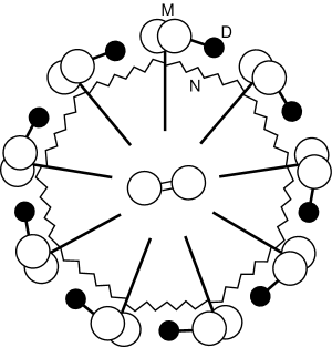
FIG. 1.: Schematic representation of the cross-section of the axoneme. Nine doublets of microtubules (M) are arranged in a cylindrical fashion, two microtubules are located in the center. Dynein motors (D) are attached to microtubule doublets and interact with a neighboring doublet. Elastic elements (N) such as nexin are indicated as springs.

How can bending waves be generated by axonemal dyneins which act internally within the axoneme? Dynein molecular motors induce relative forces between parallel elastic filaments, which are microtubule doublets. As a result of these forces, the filaments have the tendency to slide with respect to each other. If such a sliding is permitted globally, the filaments simply separate but no bending occurs. Bending results if global sliding is suppressed by rigidly connecting the filament pair in the region close to one of the two ends. In this situation, sliding is still possible locally, however only if the filaments undergo a bending deformation. This coupling of axonemal bending to local microtubule sliding has been demonstrated experimentally. In situations where the axoneme is cut at its basal end, filaments slide and in the presence of ATP separate without bending [warn81]. Small gold-beads specifically attached to microtubules in fully functioning flagella can be used to directly visualize the local relative sliding during beating [brok91].

The theoretical problem of oscillatory axonemal bending and wave patterns have been addressed by several authors. One can distinguish two principally different mechanisms to generate oscillatory forces within the axoneme: (i) Deterministic forcing: a chemical oscillator could regulate the dynein motors which are activated and deactivated periodically. In this case, the regulatory system defines a dynamical force-pattern along the axoneme and drives the system in a deterministic way [sugi82]. (ii) Self-organized beating: the axoneme oscillates spontaneously as a result of the interplay of force-generating elements and the elastic filaments [mach63, brok75, brok85, lind95]. In particular, Brokaw has studied thoroughly self-organized patterns of beating using numerical simulations of simple models [brok85, brok99]. Such models are based on the bending elasticity of the flagellum and an assumption on the coupling of motor activity to the flagellar deformations.

In the present work, we are mostly interested in self-organized beating. Our approach is conceptually different from other works as we focus on an oscillating instability of the motor-filament system. In general, spontaneous oscillations occur via a so-called Hopf-bifurcation where an initially stable quiescent state becomes unstable and starts to oscillate. There is evidence for the existence of such a dynamic instability in the axoneme. Demembranated flagella show a behavior which depends on the ATP-concentration $C_{ATP}$ in the solution. For small $C_{\rm ATP}$, the flagellum is straight and not moving. If $C_{\rm ATP}$ is increased, oscillatory motion sets in at a critical value of the ATP concentration and persists for larger concentrations [gibb75]. This implies an instability of the initial straight state with respect to a wave-like mode. Recently, it has been demonstrated using a simple model for molecular motors that a large number of motors working against an elastic element can generate oscillations via a Hopf bifurcation by a generic mechanism [juli95, juli97]. This suggests that a system consisting only of molecular motors and semiflexible filaments can in general undergo self-organized oscillations. This idea is supported by the facts that flagellar dyneins are capable of generating oscillatory motion [shin98] and that experiments suggest the existence of dynamic transitions in many-motor systems [rive98, fuji98]. Patterns of motion of cilia and flagella can be complex and embedded in three dimensional space. Many examples of propagating bending waves, however, are planar and can thus be considered as confined to two-dimensions [brok91].

In the following sections, we present a systematic study of a simplified model for the axoneme which has been introduced recently [cama99] and which captures the basic physical properties that are relevant for its dynamics. In Section II, we present a thorough analysis of the dynamics of flexible filaments driven by internal forces. This work is inspired by recent studies of the dynamics of semiflexible filaments subject to external forces [gold95, wigg98, wigg98b]. We show how the dynamic equations can be solved perturbatively and we calculate the shapes of bending waves, the velocity of swimming and the tension profile along the flagellum. In Section III, we briefly review a simple two-state model for a large number of coupled molecular motors. This model is well suited to represent the dynein molecular motors which act within the axoneme. Self-organized bending waves and oscillations via a Hopf bifurcation of the coupled motor-filament system are studied in section IV. We calculate the wave-patterns close to a Hopf bifurcation and determine the frequencies selected by the system. Finally, we discuss the relevance of our simple model to real axonemal cilia and flagella and propose experiments which could be performed to test predictions that follow from our work.

II A simple model for axonemal dynamics

The cylindrical arrangement of microtubule doublets within the axoneme can be modeled effectively as an elastic rod. Deformations of this rod lead to local sliding displacements of neighboring microtubules. Here, we consider planar deformations. In this case, the geometric coupling of bending and sliding can be captured by considering two elastic filaments (corresponding to two microtubule doublets) arranged in parallel with constant separation $a$ along the whole length of the rod. At one end, which corresponds to the basal end of an axoneme and which we call “head”, the two filaments are rigidly attached and not permitted to slide with respect to each other. Everywhere else, sliding is possible, see Fig. 2. The configurations of the system are described by the shape of the filament pair given by the position of the neutral line ${\bf r}(s)$ as a function of the arclength $s$, where ${\bf r}$ is a point in two dimensional space. The shapes of the two filaments are then given by

$${{\bf r}}_{1}(s) = {{\bf r}}(s)-a\;{\bf n}(s)/2$$ (1)

$${{\bf r}}_{2}(s) = {{\bf r}}(s)+a\;{\bf n}(s)/2\quad,$$ (2)

where ${\bf n}$ with ${\bf n}^{2}=1$ is the filament normal. The local geometry along the filament pair is characterized by the relations

$$\dot{\bf r} = {\bf t}$$ (3)

$$\dot{\bf t} = C{\bf n}$$ (4)

$$\dot{\bf n} = -C{\bf t}\quad,$$ (5)

where ${\bf t}$ denotes the normalized tangent vector and $C=\dot{\bf t}\cdot{\bf n}$ is the local curvature. Throughout this paper dots denote derivatives with respect to $s$, i.e. $\dot{\bf r}\equiv\partial_{s}{\bf r}\equiv\partial{\bf r}/\partial s$.

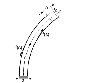
FIG. 2.: Two filaments (solid lines) ${\bf r_{1}}$ and ${\bf r_{2}}$ at constant separation $a$ are rigidly connected at the bottom end with $s=0$, where $s$ is the arclength of the neutral line ${\bf r}$ (dashed). Internal forces $f(s)$ are exerted in opposite directions, tangential to the filaments. The sliding displacement $\Delta$ at the tail is indicated.

A Bending and sliding of a filament pair

The two filaments are assumed to be incompressible and rigidly attached to each other at one end where $s=0$. Bending of the filament pair and local sliding displacements are then coupled by a geometric constraint. The sliding displacement at position $s$ along the neutral line

$$\Delta(s)\equiv\int_{0}^{s}ds^{\prime}(|\dot{\bf r}_{1}|-|\dot{\bf r}_{2}|)$$ (6)

is defined to be the difference of the total arclengths along the two filaments up to the points ${\bf r}_{1}(s)$ and ${\bf r}_{2}(s)$ which face each other along the neutral line. From Eqns. (2) and (5) follows that $\dot{\bf r}_{1,2}=(1\pm aC/2){\bf t}$ and thus

$$|\dot{\bf r}_{1,2}|=1\pm aC/2\quad.$$ (7)

Therefore,

$$\Delta=a\int_{0}^{s}ds^{\prime}C\quad$$ (8)

is given by the integrated curvature along the filament.

B Enthalpy functional

The bending elasticity of filaments (microtubules) characterizes the energetics of the filament pair. In addition to filament bending, we also have to take into account the large number of passive and active elements (e.g. nexin links and dynein molecular motors) which give rise to relative forces between neighboring microtubule doublets. These internal forces can be characterized by a coarse-grained description defining the force per unit length $f(s)$ acting at position $s$ in opposite directions on the two microtubules, see Fig. 2 (internal forces must balance). This force density is assumed to arise as the sum of active and passive forces generated by a large number of proteins. This internal force density corresponds to a shear stress within the flagellum which tends to slide the two filaments with respect to each other. A static configuration of a filament pair of length $L$ can thus be characterized by the enthalpy functional

$$G\equiv\int_{0}^{L}\left[\frac{\kappa}{2}C^{2}+f\Delta+\frac{\Lambda}{2}\dot{\bf r}^{2}\right]ds\quad.$$ (9)

Here, $\kappa$ denotes the total bending rigidity of the filaments. The incompressibility of the system is taken into account by the Lagrange multiplier function $\Lambda(s)$ which is used to enforce the constraint $\dot{\bf r}^{2}=1$ which ensures that $s$ is the arclength [gold95]. The internal force density $f$ couples to the sliding displacement $\Delta$ as described by the contribution $\int dsf\Delta$. The variation of this term under small deformations of the filament shape represents the work performed by internal stresses. Using Eq. (8) leads after a partial integration to

$$G=\int_{0}^{L}ds\left[\frac{\kappa}{2}C^{2}-aCF+\frac{\Lambda}{2}\dot{\bf r}^{2}\right]\quad,$$ (10)

where

$$F(s)\equiv-\int_{s}^{L}ds^{\prime}f\quad$$ (11)

is the force density integrated to the tail. From Eq.(10) it follows that if the internal stresses or $F$ are imposed, $G$ is minimized for a filament curvature $C=C_{0}$ where $C_{0}(s)=aF(s)/\kappa$ is a local spontaneous curvature. The internal forces therefore induce filament bending. In order to derive the filament dynamics, we determine the variation $\delta G$ with respect to variations $\delta{\bf r}$. Details of this calculation are given in Appendix A. As a result, we find

$$\frac{\delta G}{\delta{\bf r}}=\partial_{s}[\,(\kappa\dot{C}-af)\,{\bf n}-\tau{\bf t}\,\,]\quad.$$ (12)

Here,

$$\tau=\Lambda+\kappa C^{2}-aCF\quad,$$ (13)

plays the role of the physical tension. This becomes apparent since from Eq. (12) it follows that

$$\tau(s)={\bf t(s)}\cdot\left(\int_{s}^{L}ds^{\prime}\delta G/\delta{\bf r}+{\bf F}_{\em ext}(L)\right)$$ (14)

where ${\bf F}_{\em ext}(L)$ is the external force applied at the end which satisfies Eq. (25). Therefore, $\tau$ is the tangent component of the integrated forces acting on the filament.

C Dynamic equations

We derive the dynamic equation with the simplifying assumption that the hydrodynamics of the surrounding fluid can be described by two local friction coefficients $\xi_{\parallel}$ and $\xi_{\perp}$ for tangential and normal motion, respectively. The equations of motion in this case are given by [wigg98, wigg98b]

$$\partial_{t}{\bf r}=-\left(\frac{1}{\xi_{\perp}}{\bf n}{\bf n}+\frac{1}{\xi_{\parallel}}{\bf t}{\bf t}\,\right)\cdot{\frac{\delta G}{\delta{\bf r}}}\quad.$$ (15)

For the following, it is useful to introduce a coordinate system ${\bf r}=(X,Y)$ and the angle $\psi$ between the tangent ${\bf t}=(\cos\psi,\sin\psi)$ and the X-axis which satisfies $C=\dot{\psi}$. We find with Eq. (12)

$$\partial_{t}{\bf r} = \frac{1}{\xi_{\perp}}{\bf n}\,(-\kappa\stackrel{{\scriptstyle\mbox{...}}}{{\psi}}+a\dot{f}+\dot{\psi}\tau)$$ (16)

$$+ \frac{1}{\xi_{\parallel}}{\bf t}\,(\kappa\dot{\psi}\ddot{\psi}-a\dot{\psi}f+\dot{\tau})\quad.$$ (17)

Noting that $\partial_{t}\dot{\bf r}={\bf n}\partial_{t}\psi$, we obtain an equation of motion for $\psi(s)$ alone:

$$\partial_{t}\psi = \frac{1}{\xi_{\perp}}(-\kappa\stackrel{{\scriptstyle\mbox{....}}}{{\psi}}+a\ddot{f}+\dot{\psi}\dot{\tau}+\tau\ddot{\psi})$$ (18)

$$+ \frac{1}{\xi_{\parallel}}\dot{\psi}(\kappa\dot{\psi}\ddot{\psi}-af\dot{\psi}+\dot{\tau})\quad.$$ (19)

The tension $\tau$ is determined by the constraint of incompressibility $\partial_{t}\dot{\bf r}^{2}=2{\bf t}\cdot\partial_{t}\dot{\bf r}=0$. This condition and Eq. (17) leads to a differential equation for the tension profile:

$$\ddot{\tau}-\frac{\xi_{\parallel}}{\xi_{\perp}}\dot{\psi}^{2}\tau=a\partial_{s}(\dot{\psi}f)-\kappa\partial_{s}(\dot{\psi}\ddot{\psi})+\frac{\xi_{\parallel}}{\xi_{\perp}}\dot{\psi}(a\dot{f}-\kappa\stackrel{{\scriptstyle\mbox{...}}}{{\psi}})\quad.$$ (20)

Eqns. (19) and (20) determine the filament dynamics. The filament shape follows from

$${\bf r}(s,t)={\bf r}(0,t)+\int_{0}^{s}(\cos\psi,\sin\psi)ds^{\prime}\quad,$$ (21)

where ${\bf r}(0,t)$ can be obtained from Eq. (17) evaluated at $s=0$.

D Boundary Conditions

The filament dynamics depends on the imposed boundary conditions. The variation $\delta G$ has contributions at the boundaries which can be interpreted as externally applied forces ${\bf F}_{\rm ext}$ and torques $T_{\rm ext}$ acting at the ends, see Appendix A. At the head with $s=0$,

$${\bf F}_{\rm ext} = (\kappa\dot{C}-af){\bf n}-\tau{\bf t}$$ (22)

$$T_{\rm ext} = -\kappa C-a\int_{0}^{L}ds^{\prime}f\quad.$$ (23)

Similarly, at the tail for $s=L$,

$${\bf F}_{\rm ext} = (-\kappa\dot{C}+af){\bf n}+\tau{\bf t}$$ (24)

$$T_{\rm ext} = \kappa C\quad.$$ (25)

If constraints on the positions and/or angles are imposed at the ends, forces and torques have to be applied to satisfy these constraints. In the following, we will discuss different boundary conditions as specified in Table I:

Case A is the situation of a filament with clamped head, i.e. both the tangent and the position at the head are fixed, the tail is free. Case B is a filament with fixed head, i.e. the tangent at the head can vary. The situation of a swimming sperm corresponds to case C where the friction force of a viscous load attached at the head is taken into account, the head is otherwise free. As an example of a situation with an external force ${\bf F}_{\rm ext}(L)$ applied at the tail we consider Case D. For simplicity, we assume a force parallel to the (fixed) tangent at the head.

boundary	head $s=0$		tail $s=L$
condition
A	$\partial_{t}{\bf r}={\bf 0}$	$\partial_{t}{\bf t}={\bf 0}$	${\bf F}_{\rm ext}={\bf 0}$	$T_{\rm ext}=0$
B	$\partial_{t}{\bf r}={\bf 0}$	$T_{\rm ext}=0$	${\bf F}_{\rm ext}={\bf 0}$	$T_{\rm ext}=0$
C	${\bf F}_{\rm ext}=-\zeta\partial_{t}{\bf r}$	$T_{\rm ext}=0$	${\bf F}_{\rm ext}={\bf 0}$	$T_{\rm ext}=0$
D	$\partial_{t}{\bf r}={\bf 0}$	$\partial_{t}{\bf t}={\bf 0}$	${\bf F}_{\rm ext}\neq{\bf 0}$	$T_{\rm ext}=0$

TABLE I.: Different boundary conditions studied. (A) clamped head, free tail; (B) fixed head, free tail; (C) swimming flagellum with viscous load $\zeta$; (D) clamped head, external force applied at the tail.

E Small deformations

In the absence of internal forces $f$, the filament relaxes passively to a straight rod with $\dot{\psi}=0$, i.e. $\psi$ constant. Without loss of generality, we choose $\psi=0$ in this state which implies that straight filament is parallel to the $X$-axis. Internal stresses $f(s)$ induce deformations of this straight conformation. For small internal stresses, we can perform a systematic expansion of the filament dynamics in powers of the stress amplitude.

We introduce a dimensionless parameter $\epsilon$ which scales the amplitudes of the internal stresses, $f(s,t)=\epsilon f_{1}(s,t)$, where $f_{1}$ is an arbitrary stress distribution. We can now solve the dynamic equations (19) and (20) perturbatively by writing

$$\psi = \epsilon\psi_{1}+\epsilon^{2}\psi_{2}+O(\epsilon^{3})$$ (26)

$$\tau = \tau_{0}+\epsilon\tau_{1}+\epsilon^{2}\tau_{2}+O(\epsilon^{3})\quad,$$ (27)

which allows us to determine the coefficients $\psi_{n}(s,t)$ and $\tau_{n}(s,t)$. This procedure is described in Appendix B. We find that $\psi_{2}$ and $\tau_{1}$ always vanish and $\tau_{0}=\sigma$ is a constant tension which is equal to the $X$-component of the external force applied at the end. Note, that for boundary conditions A-C, $\sigma=0$. The filament shape is thus characterized by the behavior of $\psi_{1}(s,t)$ which obeys

$$\xi_{\perp}\partial_{t}\psi_{1}=-\kappa\stackrel{{\scriptstyle\mbox{....}}}{{\psi_{1}}}+\sigma\ddot{\psi_{1}}+a\ddot{f_{1}}\quad.$$ (28)

In order to discuss the filament motion in space, we define the average velocity of swimming

$$\bar{\bf v}=\lim_{t\rightarrow\infty}\frac{1}{t}\int_{0}^{t}dt^{\prime}\partial_{t}{\bf r}$$ (29)

which is independent of $s$. This velocity is different from zero only in the case of boundary condition C. We choose the $X$-axis parallel to $\bar{\bf v}$ and introduce a coordinate system $(x,y)$ which moves with the filament

$$(x,y)=(X-\bar{v}t,Y)\quad,$$ (30)

where $\bar{v}=\pm|\bar{\bf v}|$ and the sign depends on whether motion is towards the positive or negative $X$-direction, see Fig. 3. It is useful to introduce the transverse and longitudinal deformations $h$ and $u$, respectively, which satisfy

$$(x,y)=\left(s+u(s),h(s)\right)$$ (31)

and which vanish for $\epsilon=0$. The quantities $h$, $u$ and $\bar{v}$ can be calculated perturbatively in $\epsilon$, see Appendix B. To second order in $\epsilon$ transverse motion satisfies

$$\xi_{\perp}\partial_{t}h=-\kappa\partial_{s}^{4}h+\sigma\partial_{s}^{2}h+a\partial_{s}f$$ (32)

Longitudinal displacements satisfy

$$u(s)=u(0)-\frac{1}{2}\int_{0}^{s}(\partial_{s}h)^{2}ds^{\prime}$$ (33)

The boundary conditions for $h(s)$ are given in table II.

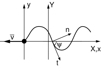
FIG. 3.: Resting frame $(X,Y)$ and frame $(x,y)$ moving with the filament at velocity $\bar{v}$. The tangent ${\bf t}$ and the normal ${\bf n}$ are indicated, the angle between the $X,x$-axis and ${\bf t}$ is denoted $\psi$.

F Swimming

The velocity of swimming $\bar{v}$ can be calculated perturbatively in $\epsilon$. We consider for simplicity periodic internal stresses with frequency $\omega$ given by

$$f(s,t)=\tilde{f}(s)^{i\omega t}+\tilde{f^{*}}(s)e^{-i\omega t}\quad$$ (34)

which after long time leads to periodic filament motion

$$h(s,t)=\tilde{h}(s)e^{i\omega t}+\tilde{h^{*}}(s)e^{-i\omega t}$$ (35)

where $\tilde{h}$ satisfies according to Eq. (32)

$$\kappa\partial_{s}^{4}\tilde{h}-\sigma\partial_{s}^{2}\tilde{h}+\xi_{\perp}i\omega\tilde{h}=a\partial_{s}\tilde{f}\quad.$$ (36)

boundary	head $s=0$		tail $s=L$
condition	$F=-\int_{0}^{L}dsf$		$\partial_{s}^{2}h=0$
A	$h=0$	$\partial_{s}h=0$	$\kappa\partial_{s}^{3}h=af$
B	$h=0$	$\kappa\partial_{s}^{2}h=aF$	$\kappa\partial_{s}^{3}h=af$
C	$\zeta\partial_{t}h=af-\kappa\partial_{s}^{3}h$	$\kappa\partial_{s}^{2}h=aF$	$\kappa\partial_{s}^{3}h=af$
D	$h=0$	$\partial_{s}h=0$	$\kappa\partial_{s}^{3}h$
			$-\sigma\partial_{s}h=af$

TABLE II.: Boundary conditions for small amplitude motion. (A) clamped head, free tail; (B) fixed head, free tail; (C) swimming flagellum with viscous load $\zeta$; (D) clamped head, external force applied at the tail.

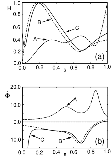
FIG. 4.: Fundamental modes of filament motion $\tilde{h}_{1}(s)=He^{-i\phi}$ close to a Hopf bifurcation are displayed for an oscillation frequency of about $50Hz$ and boundary conditions A-C. In case C, a viscous load $\zeta\simeq 5.10^{-8}Ns/m$ acts at the head. (a) Amplitude $H$ in arbitrary units as a function of arclength $s$. (b) Same plot for the gradient of the phase $\dot{\phi}$.

Writing $\tilde{h}=He^{-i\phi}$ where $H$ and $\phi$ denote the amplitude and phase, respectively, filament motion can be expressed as

$$h(s,t)=H(s)\cos(\omega t-\phi(s))\quad,$$ (37)

which represents bending waves for which $v_{p}=\omega/\dot{\phi}$ can be interpreted as the local wave propagation velocity. Examples of bending waves for self-organized beating discussed in section IV are displayed in Figs. 4 and 5. For a freely oscillating filament with a viscous load of friction coefficient $\zeta$ attached (case C), we find an average propulsion velocity $\bar{v}=V_{0}/(1+\zeta/\xi_{\parallel}L)$ where

$$V_{0}=-\left(\frac{\xi_{\perp}}{\xi_{\parallel}}-1\right)\frac{\omega}{2L}\int_{0}^{L}dsH^{2}\dot{\phi}\quad,$$ (38)

is the velocity for $\zeta=0$. Eq. (38) which is correct to second order in $\epsilon$ reveals that motion is only possible if the filament friction is anisotropic $\xi_{\parallel}/\xi_{\perp}\neq 1$ and if a wave is propagating, $\dot{\phi}\neq 0$. This is consistent with earlier work on swimming [tayl51, purc77, ston96]. For a rod-like filament with $\xi_{\parallel}<\xi_{\perp}$, swimming motion is opposite to the direction of wave propagation.

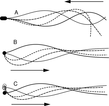
FIG. 5.: Filament shapes in the $(x,y)$ plane that correspond to the modes displayed in Fig. 4. Snapshots taken at different times to illustrate bending waves are shown for boundary conditions A-C. The arrows indicate the direction of wave propagation.

III Internal forces generated by molecular motors

The filament dynamics is driven by internal stresses $f(s,t)$ generated by a large number of dynein motors and passive elements. We describe the properties of a force-generating system using a simplified two-state model.

A Two state model for molecular motors

We briefly review the two-state model for a large number of motor molecules attached to a filament which slides with respect to a second filament [juli95, juli97b]. Each motor is assumed to have two different chemical states, a strongly bound state $1$ and a weakly bound state or detached state $2$. The interaction between a motor and a filament in states $1$ and $2$ is characterized by energy landscapes $W_{1}(x)$ and $W_{2}(x)$, where $x$ denotes the position of a motor along the filament. The potentials reflect the symmetry of the filaments: they are periodic with period $l$, $W_{i}(x)=W_{i}(x+l)$ and are spatially asymmetric, $W_{i}(x)\neq W_{i}(-x)$. In the presence of ATP which is the chemical fuel that drives the system, the motors are assumed to undergo transitions between states. The corresponding transition rates are denoted $\omega_{1}$ for detachments and $\omega_{2}$ for attachments. We introduce the relative position $\xi$ of a motor with respect to the potential period where $x=\xi+nl$, $0\leq\xi<l$ and $n$ is an integer. The probability to find a motor in state $i$ at position $\xi$ at time $t$ is denoted $P_{i}(\xi,t)$, $P_{1}+P_{2}$ is normalized within one period. The dynamic equations of the system are given by

$$\partial_{t}P_{1}+v\partial_{\xi}P_{1} = -\omega_{1}P_{1}+\omega_{2}P_{2}$$ (39)

$$\partial_{t}P_{2}+v\partial_{\xi}P_{2} = \omega_{1}P_{1}-\omega_{2}P_{2}\quad.$$ (40)

The sliding velocity $v=\partial_{t}x$ is determined by the force-balance

$$f=\lambda v+\rho\int_{0}^{l}(P_{1}\partial_{\xi}W_{1}+P_{2}\partial_{\xi}W_{2})d\xi\ +Kx\quad.$$ (41)

Here, the coefficient $\lambda$ describes the total friction per unit length in the system. The number density of motors along the filament is denoted by $\rho$ and $f$ is the force per unit length generated by the system. The elastic modulus per unit length $K$ occurs in presence of elastic elements such as nexins. If motors have an incommensurate arrangement compared to the filament periodicity, $P_{1}+P_{2}=1/l$ and the equations simplify and can be expressed by $P_{1}$ alone

$$\partial_{t}P_{1} + v\partial_{\xi}P_{1}=-(\omega_{1}+\omega_{2})P_{1}+\omega_{2}/l$$ (42)

$$f = \lambda v+\rho\int_{0}^{l}P_{1}\partial_{\xi}\Delta W+Kx$$ (43)

where $\Delta W=W_{1}-W_{2}$.

B Molecular motors coupled to a filament pair

The two state model for a large number of motors is well suited to represent the internal forces acting within the axoneme. We assume that at any position $s$ an independent two-state model described by Eq. (43) is located which generates the internal force density $f(s)$. The filament sliding displacement is identified with the motor displacement, $\Delta\equiv x$. Note, that here we neglect for simplicity fluctuations which arise from the chemical activity of a finite number of force generators and we assume homogeneity of all properties along the axonemal length. The energy source of the active system is the chemical activity characterized by the transition rates $\omega_{1}$ and $\omega_{2}$, the generated forces induce bending deformations of the filaments.

The dynamic equations (43) represent a nonlinear active system which generates time-dependent forces. Since we will study periodic motion, we can express forces and displacements by a Fourier expansion

$$f(t) = \sum_{n}f_{n}e^{in\omega t}$$ (44)

$$\Delta(t) = \sum_{n}\Delta_{n}e^{in\omega t}\quad.$$ (45)

The relation between force amplitudes $f_{n}$ and amplitudes of sliding displacements $\Delta_{n}$ can in general be expressed in powers of the amplitudes $\Delta_{n}$ [juli97]

$$f_{n}=F^{(1)}_{nk}\Delta_{k}+F^{(2)}_{nkl}\Delta_{k}\Delta_{l}+O(\Delta_{k}^{3})\quad.$$ (46)

Here, the summation over common indices is implied. The coefficients $F^{(n)}$ are calculated for the two-state model in Appendix C. However, Eq. (46) is more general and characterizes a whole class of active nonlinear mechanical systems.

C Symmetry considerations

The interaction of the motors with the two filaments is asymmetric. Motors are rigidly connected to one of the filaments and slide along the second. In addition, the filaments are polar and filament sliding is induced by motors towards one particular end of the two filaments. As a consequence, the system has a natural tendency to create bending deformations with one particular sign of the curvature. Exchanging the role of the two filaments rthis sign of bending deformations. This broken symmetry does however not reflect the symmetry of the axoneme which is symmetric with respect to all microtubule doublets. Each of the nine microtubule doublet within the cylindrical arrangement of the axoneme play identical roles and interact with rigidly attached motors as well as with motors which slide along their surfaces. If all motors generate a constant force, there is consequently no resulting bending deformation since all bending moments cancel by symmetry.

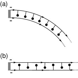
FIG. 6.: Asymmetric (a) and symmetric (b) motors/filament pair. The arrows indicate the polarity of the filaments. In case (a), spontaneous bending occurs. In case (b) both filaments play identical roles, no spontaneous bending occurs.

In order to introduce this axonemal symmetry in our two-dimensional model, we assume that both filaments have motors which are rigidly attached and which slide on the second filament, see Fig. 6. The consequence of this symmetry is that the filament polarity becomes unimportant. Exchanging the role of the two filaments is equivalent to replacing the sliding displacement $\Delta$ of motors by $-\Delta$. Therefore, in the context of the two-state model this symmetrization is equivalent to the requirement that energy landscapes $W_{i}(x)$ and transition rates $\omega_{i}(x)$ are symmetric functions with respect to $x\rightarrow-x$. As a consequence of this symmetry, there is no preferred direction of bending. In the following, we adopt this choice of a symmetric motor/filament pair. If we use the expansion given in Eq. (46), this symmetry implies that all even coefficients $F^{(2n)}=0$.

D Linear response function

The perturbative treatment to study small filament deformations introduced in section II can be naturally extended to the coupled motor-filament situation using the expansion (46). Up to second order in $\epsilon$, only the linear response coefficient of the active system plays a role which for the two-state model is given by $F^{(1)}_{nk}=\chi\delta_{nk}$ with

$$\chi=K+\lambda i\omega-\rho\int_{0}^{l}d\xi\,\partial_{\xi}\Delta W\frac{\partial_{\xi}R}{\alpha+i\omega}i\omega\quad.$$ (47)

Here, we have introduced $R\equiv\omega_{2}/\alpha l$ and $\alpha=\omega_{1}+\omega_{2}$. Higher order terms $F^{(2n+1)}$ have to be taken into account if the third or higher order in $\epsilon$ is considered. The linear response function $\chi$ as well as nonlinear coefficients can be calculated most easily for a simple choice of symmetric potential and transition rates

$$\Delta W(\xi) = U\cos(2\pi\xi/l)$$ (48)

$$\omega_{1}(\xi) = \beta-\beta\cos(2\pi\xi/l)$$ (49)

$$\omega_{2}(\xi) = \alpha-\beta+\beta\cos(2\pi\xi/l)$$ (50)

where $\alpha$ and $\beta$ are $\xi$-independent rate constants. For this convenient choice

$$\chi(\Omega,\omega)=K+i\lambda\omega-\rho k\Omega\frac{i\omega/\alpha+(\omega/\alpha)^{2}}{1+(\omega/\alpha)^{2}}\quad,$$ (51)

where $k\equiv U/l^{2}$ is the cross-bridge elasticity of the motors. We have introduced the dimensionless parameter $\Omega=2\pi^{2}\beta/\alpha$ with $0<\Omega<\pi^{2}$ which plays the role of a control parameter of the motor-filament system, $\alpha$ is a characteristic ATP cycling rate.

IV Self-organized beating via a Hopf bifurcation

A Hopf-bifurcation is an oscillating instability of an initial non-oscillating state which occurs for a critical value $\Omega_{c}$ of a control parameter. For $\Omega<\Omega_{c}$, the system is passive and not moving, while for $\Omega>\Omega_{c}$ it exhibits spontaneous oscillations. As we demonstrate below, self-organized oscillations of the driven filament pair are a natural consequence of its physical properties. The control parameter $\Omega$ is in our two-state model a ratio of chemical rates of the ATP hydrolysis cycle. In an experimental situation, it could be varied e.g. by changing the ATP concentration. If the molecular motors are regulated by some other ion concentration such as e.g. $Ca^{2+}$, this concentration could also play the role of the control parameter.

A Generic aspects

For oscillations in the vicinity of a Hopf-bifurcation, filament deformations are small and we can thus use Eq. (32) to describe the filament dynamics. The force amplitude $\tilde{f}$ can be obtained from the expansion

$$\tilde{f}=\chi(\Omega,\omega)\tilde{\Delta}+O(\tilde{\Delta}^{3})\quad$$ (52)

in the amplitude of sliding displacements. In addition, this amplitude is related to the filament shape:

$$\Delta(s)=a(\partial_{s}h(s)-\partial_{s}h(0))+O(h^{3})\quad.$$ (53)

With Eq. (36), we find that spontaneously oscillating modes $\tilde{h}(s)$ at frequency $\omega$ are to linear order near the bifurcation solutions to

$$\kappa\partial_{s}^{4}\tilde{h}-\sigma\partial_{s}^{2}\tilde{h}+\xi_{\perp}i\omega\tilde{h}=a^{2}\chi\partial_{s}^{2}\tilde{h}$$ (54)

Note that this equation is general and its structure does not depend on the specific model chosen for the force generating elements. Boundary conditions corresponding to cases A-D follow from Table II by replacing $h\rightarrow\tilde{h}$, $\partial_{t}h\rightarrow i\omega\tilde{h}$ and $f\rightarrow\tilde{f}=a\chi(\partial_{s}\tilde{h}-\partial_{s}\tilde{h}(0))$.

As discussed in Appendix D, Eq. (54) has the structure of an eigenvalue problem, with $\chi$ playing the role of a complex eigenvalue. For every choice of parameters, there exists an infinite set of nontrivial solutions $\tilde{h}_{n}$ to Eq. (54) if $\chi$ is equal to the corresponding eigenvalue $\chi_{n}$, $n=1,2,..$. We order these values according to their amplitude: $|\chi_{n}|\leq|\chi_{n+1}|$. The functional dependence of the Eigenvalues $\chi_{n}$ on the model parameters is completely determined by dimensionless functions $\bar{\chi}_{n}(\bar{\sigma},\bar{\omega})$ according to

$$\chi_{n}=\frac{\kappa}{L^{2}a^{2}}\bar{\chi}_{n}(\bar{\sigma},\bar{\omega})\quad,$$ (55)

where $\bar{\sigma}\equiv\sigma L^{2}/\kappa$ and $\bar{\omega}\equiv\omega\xi_{\perp}L^{4}/\kappa$ are a dimensionless tension and frequency, respectively.

The existence of discrete eigenvalues reveals that only particular values of the linear response function of the active material are consistent with being in the vicinity of a Hopf-bifurcation. If the actual value of $\chi(\Omega,\omega)$ of the system differs from one of the eigenvalues $\chi_{n}$, the system is either not oscillating, or it oscillates with large amplitude for which higher order terms in $\epsilon$ cannot be neglected. An important consequence of this observation is that the modes $\tilde{h}_{n}$ of filament beating close to a Hopf-bifurcation can be calculated without knowledge of the properties of the active elements. Not even knowledge of the linear response coefficient is required since it follows as an eigenvalue at the bifurcation. Therefore, filament motion close to a Hopf bifurcation has generic or universal features which do not depend on details of the problem such as the structural complexity within the axoneme. The motion is given by one of the modes $\tilde{h}_{n}$ which only depend on $\bar{\sigma}$ and $\bar{\omega}$.

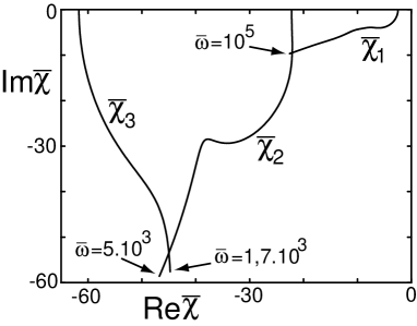
FIG. 7.: (a) Eigenvalues $\bar{\chi}_{n}$ for boundary conditions B. Each eigenvalue is represented by a line which traces the locations of $\bar{\chi}_{n}$ in the complex plane for varying reduced frequency $\bar{\omega}$. The lines begin for $\bar{\omega}=0$ on the real axis, the value of $\bar{\omega}$ at the other ends are indicated.

Fig. 4 displays the amplitude $H$ and the gradient of the phase $\dot{\phi}$ of the fundamental mode $\tilde{h}_{1}=He^{-i\phi}$. Note, that we use arbitrary units for $H$ since the amplitude of $\tilde{h}(s)$ is not determined by Eq. (54). Corresponding filament shapes represented according to Eq. (31) in the $(x,y)$ plane, are displayed in Fig. 5 for boundary conditions A-C as snapshots taken at different times. The oscillation amplitudes are chosen in such a way that the maximal value of $\psi\simeq\pi/2$. The direction of wave propagation depends on the boundary conditions. For clamped head (case A), waves propagate towards the head whereas for fixed or free head (cases B and C), they propagate towards the tail. The positions of the lowest eigenvalues $\bar{\chi}_{n}$ in the complex plane for boundary conditions B are displayed in Fig. 7 for $\bar{\sigma}=0$ and varying $\bar{\omega}$.

B Selection of eigenmodes and frequency

In order to determine which of the modes $\tilde{h}_{n}$ is selected and at what frequency $\omega$ the system oscillates at the bifurcation point, explicit knowledge of the linear response function $\chi(\Omega,\omega)$ is necessary. As a simple example, we use $\chi$ as given by Eq. (51) for a two-state model. For $\Omega=0$, $\chi=K+i\lambda\omega$ which is a passive viscoelastic response. In this case, no spontaneous motion is possible which can be seen by the fact that all eigenvalues $\bar{\chi}_{n}$ have negative real and imaginary parts which cannot be matched by the linear response of a passive system. If $\Omega$ is increased, we are interested in a critical point $\Omega=\Omega_{c}$ for which the straight filament configuration becomes unstable. This happens as soon as the linear response function $\chi$ matches for a particular frequency $\omega=\omega_{c}$ one of the complex eigenvalues,

$$\frac{\kappa}{a^{2}L^{2}}\bar{\chi}_{n}(\bar{\sigma},\bar{\omega}_{c})=\chi(\Omega_{c},\omega_{c})\quad,$$ (56)

where $\bar{\omega}_{c}=\xi_{\perp}L^{4}\omega_{c}/\kappa$. Since $\chi$ is complex, both the real and the imaginary part of Eq. (56) represent independent conditions. Therefore, Eq. (56) determines both the critical point $\Omega_{c}$ as well as the selected frequency $\omega_{c}$. The selected mode $n$ is the first mode (beginning from $\Omega=0$) to satisfy this condition. Since $|\chi(\Omega,\omega)|$ typically increases with increasing $\Omega$, the instability occurs almost exclusively for $n=1$ since $|\bar{\chi}_{1}|$ has been defined to have the smallest value. For $\Omega>\Omega_{c}$, but close to the transition, the system oscillates spontaneously with frequency $\omega_{c}$. The shapes of filament beating are characterized by the corresponding mode $\tilde{h}_{n}(s)$ whose amplitude is determined by nonlinear terms. For the case of a continuous transition, the deformation amplitude increases as $|\tilde{h}_{n}|\sim(\Omega-\Omega_{c})^{1/2}$.

C Axonemal vibrations for different lengths

We choose the parameters of our model to correspond to the axonemal structure. We estimate the bending rigidity $\kappa\simeq 4\cdot 10^{-22}$Nm² which is the rigidity of about 20 microtubules. Furthermore, we choose a microtubule separation $a\simeq 20$nm, motor density $\rho\simeq 5\cdot 10^{8}$m^-1, friction per unit length $\lambda\simeq 1$kg/ms, rate constant $\alpha\simeq 10^{3}$s^-1, cross-bridge elasticity $k\simeq 10^{-3}$N/m and a perpendicular friction $\xi_{\perp}\simeq 10^{-3}$kg/ms which is of the order of the viscosity of water. A rough estimate of the elastic modulus per unit length associated with filament sliding can be obtained by comparing the number of dynein heads to the number of nexin links within the axoneme. This suggests that $K$ is relatively small, $K{<\atop\sim}k\rho/10$.

The selected frequency $\omega_{c}$ at the bifurcation point for case B is shown in Fig. 8 as a function of the axoneme length for $K=0$. For small lengths, the oscillation frequency is large and increases as $L$ decreases. In this high-frequency regime, which occurs for $L{<\atop\sim}10\mu$m, the system vibrates in a mode with no apparent wave propagation. For $L{>\atop\sim}10\mu$m the frequency is only weakly $L$-dependent and the system propagates bending waves of a wave-length shorter than the filament length.

The limit of small lengths corresponds to small $\bar{\omega}$ and can be studied analytically. For $\bar{\sigma}=0$, the eigenvalue $\chi_{1}$ is given to linear order in $\bar{\omega}$ by $\bar{\chi}_{1}\simeq-\pi^{2}/4-i\gamma\bar{\omega}$. The coefficient $\gamma$ depends on boundary conditions but not on any model parameters. For a clamped head (A), $\gamma\simeq 0.184$, for a fixed head (B), $\gamma\simeq 0.008$, see Appendix D. The criterion for a Hopf bifurcation for small $L$ is

$$\chi(\Omega_{c},\omega_{c})\simeq-\frac{\pi^{2}\kappa}{4a^{2}L^{2}}-i\gamma\frac{\xi_{\perp}\omega_{c}L^{2}}{a^{2}}$$ (57)

Together with Eq.(51), we find the critical frequency

$$\omega_{c}\simeq\frac{\pi}{2L^{2}}\left(\frac{\kappa\alpha}{\gamma\xi_{\perp}}\right)^{1/2}\left[\frac{1+(L/L_{K})^{2}}{1+(L_{\lambda}/L)^{2}}\right]^{1/2}\quad,$$ (58)

where $L_{K}\equiv(\pi^{2}\kappa/4Ka^{2})^{1/2}$ and $L_{\lambda}\equiv(\lambda a^{2}/\gamma\xi_{\perp})^{1/2}$ are two characteristic lengths. For $K$ and $\lambda$ small, $L_{K}\gg L\gg L_{\lambda}$ and the critical frequency behaves as $\omega_{c}\sim 1/L^{2}$.

FIG. 8.: Oscillation frequency $\omega_{c}/2\pi$ at the bifurcation point as a function of the axoneme length $L$ for boundary conditions B and model parameters as given in the text. The insets show characteristic patterns of motion for small and large lengths.

The critical value of the control-parameter for small $L$ is given by

$$\Omega_{c}\simeq\frac{\kappa\pi^{2}}{4a^{2}\rho kL^{2}}+\frac{K+\lambda\alpha}{\rho k}+\frac{\alpha\gamma\xi_{\perp}L^{2}}{\rho ka^{2}}\quad.$$ (59)

For axoneme lengths below a characteristic value, $L<L_{\rm min}$, the condition $\Omega_{c}\leq\pi^{2}$ is violated. Therefore, oscillations exist only for $L>L_{\rm min}$. If $(K+\lambda\alpha)/\rho k\ll 1$, $L_{min}\simeq\sqrt{\kappa/4a^{2}\rho k}\simeq 1\mu$m for our choice of the parameters. The maximal frequency of oscillations occurs for $L=L_{\rm min}$. Within the range of lengths between $1\mu m$ and $50\mu m$, we find frequencies $\omega_{c}/2\pi$ which vary between tens of Hz and about $20kHz$. The parameters chosen in Fig. 8 lead to frequencies above $150Hz$. Lower frequencies are obtained for larger values of the friction $\lambda$ or smaller chemical rate $\alpha$.

D Effect of external forces applied at the tail

In the presence of an external force applied at the end $\bar{\sigma}\neq 0$ and the filament pair is under tension. The eigenvalues $\bar{\chi}_{n}$ depend on $\bar{\sigma}$, therefore the tension affects shape and frequency of an unstable mode. Inspection of Eq. (54) suggests that the tension $\sigma$ can be interpreted as an additive contribution to the linear response coefficient $\chi\rightarrow\chi+\sigma/a^{2}$. Taking into account the boundary conditions complicates the situation, the $\bar{\sigma}$-dependence of the eigenvalues is in general nontrivial. However, for a filament with clamped head and a force applied at the tail parallel to the tangent at the head (case D) the effect of tension can be easily studied. In this particular case, the tension leads to the same contribution to $\chi$ both in Eq. (54) and in the boundary conditions and the eigenvalues thus depend linearly on $\sigma$:

$$\bar{\chi}_{n}(\bar{\sigma},\bar{\omega})=\bar{\chi}_{n}(0,\bar{\omega})-\bar{\sigma}\quad.$$ (60)

Since the tension corresponds to a change of the real part of $\chi$, its presence has the same effect on filament motion as an increase of the elastic modulus $K$ per unit length in Eq. (51) by $\sigma/a^{2}$. Therefore, we can include the effects of tension on the critical frequency in Eq. (58) by replacing $K\rightarrow K+\sigma/a^{2}$ which reveals that in those regimes where the frequency depends on $K$, it will increase for increasing tension. The critical value of the control parameter $\Omega_{c}$ is a function of the tension, with Eq. (59), we find

$$\Omega_{c}(\sigma)=\Omega_{c}(0)+\frac{1}{\rho ka^{2}}\sigma\quad.$$ (61)

For our choice of parameters, $\rho ka^{2}\simeq 200$pN which indicates that forces of the order of $10^{2}pN$ should have a significant effect on the bifurcation. Furthermore, Eq. (61) indicates that the tension $\sigma$ can play the role of a second control parameter for the bifurcation. Consider a tensionless filament oscillating close to the bifurcation for $\Omega>\Omega_{c}(0)$. If a tension is applied, the critical value $\Omega_{c}(\sigma)$ increases until the system reaches for a critical tension $\sigma_{c}$ a bifurcation point with $\Omega_{c}(\sigma_{c})=\Omega$ and the system stops oscillating.

V Discussion

In the previous sections, we have shown that many aspects of axonemal eating can be described by a simple model based on the idea of local sliding of microtubule doublets driven by molecular motors inside the axoneme. This model represents a class of physical systems termed internally driven filaments [cama99] which have characteristic properties that are closely linked to the geometric constraint that couples global bending and local filament sliding.

Our work shows that axonemal beating can be studied both numerically and analytically using a coarse-grained description which ignores many details of the proteins involved and is based on effective material properties such as bending rigidities, internal friction coefficient and elastic modulus per unit length as well as the frequency dependent linear response function of the active elements. Our main results are: (i) The filament pair introduces a geometric coupling of the active elements at different position along the filaments. This coupling is suited for the generation of periodic beating motion by a general self-organization mechanism of the system. (ii) The generation of oscillations and propagating bending waves occurs via a Hopf bifurcation for a critical value of a control-parameter such as the ATP concentration. The patterns of motion generated close to this bifurcation can be calculated without any knowledge of the internal force generating mechanism if the oscillation frequency is known. (iii) The frequency depends on chemical rates of the motors, coefficients of internal elasticities and frictions, the solvent viscosity and the microtubule rigidity. Our calculations using a simple two-state model for molecular motors suggest significant variations of the oscillation frequency if the axonemal length is varied. Short axonemes are predicted to be able to oscillate at frequencies of several kHz. This fact is particularly interesting in the case of kinocilia which are located in the hair bundles of many mechanosensitive cells that are involved in the detection of sounds. If cilia are able to vibrate at high frequencies, this suggests that the kinocilium could play as active role in sound detection [cama00]. (iv) Forces applied to the axoneme can be an important tool to study the mechanism of force generation. An external force can play the role of a second control parameter for the bifurcation which has a stabilizing effect for increasing forces.

These results have been obtained using several simplifying assumptions. Our model represents the solvent hydrodynamics by an anisotropic local friction acting on the rod-like filament. This approach ignores hydrodynamic interactions between different parts of the filament which lead to logarithmic corrections. These hydrodynamic effects do not change the basic physics but can lead to corrections to the numerical results. It is straightforward to generalize our model to incorporate the effects of hydrodynamic interaction, but this does not change our results qualitatively. A more serious simplification of our model is the restriction to a two-dimensional system and to filament configurations which are planar. This choice is motivated by the fact that observed bending waves of flagella are planar in many cases [brok91]. If filament configurations are planar then our model applies and is complete. However, this model cannot explain why motion is confined to a plane and it misses all non-planar modes of beating. In order to address such questions, a three dimensional generalizations have to be used. Such generalizations introduce additional aspects. In particular, torsional deformations become relevant. The local sliding displacements depend in the three dimensional case both on bending and torsional deformations and the full torsional dynamics has to be accounted for in the dynamic equations. Finally, we have restricted most calculations to the limit of small deformations which corresponds to filament shapes that are almost straight. This regime has several important features. The filament dynamics can be studied by an analytic approach by a systematic expansion in the deformation amplitude. This allows us to characterize linear and nonlinear terms both for the filament dynamics as well as for the properties of the active elements. Patterns of motion close to a Hopf bifurcation are fully characterized by the linear terms of this expansion. These linear terms are given by the structure of the problem and their form does not depend on molecular details of the system. For example, most details of the operation of the molecular motors are unimportant for the shape of the filament oscillations at the bifurcation, only the linear response function of the active material plays a role.

If filament beating with larger amplitude is of interest, nonlinearities become relevant. Nonlinearities arise due to nonlinear geometric terms in the bending energy or via non-Hookian corrections of the elasticity. Furthermore, nonlinearities in the force-generation process of molecular motors exist. All these nonlinearities determine the large amplitude motion and could give rise to new types of behavior such as additional dynamic instabilities. However, in contrast to the linear terms, the form of the dominant nonlinearities does depend on structural details of the axoneme. Therefore, an analysis of large amplitude motion is difficult and knowledge of the nature of the dominating nonlinearities is required. However, if no new instabilities after the initial Hopf-bifurcation occur, the principal effect of nonlinear terms is to fix the amplitude of propagating waves. We therefore expect that propagating waves with larger amplitude are in many cases well approximated by our calculation to linear order.

Our work shows that propagating bending waves and oscillatory motion of internally driven filaments can occur naturally by a simple physical mechanism. Complex biochemical networks to control the system are not required for wave propagation to occur. This suggests that the basic axonemal structure intrinsically has the ability to oscillate. Biochemical regulation systems are thus expected to control this activity on a higher level but are not responsible for oscillations. Our work shows that experimental studies of axonemal beating close to a Hopf bifurcation would be very valuable. Such experiments could be e.g. performed by using demembranated flagella and ATP concentrations not far from the level where beating sets in. The observed behavior close to the bifurcation would give insight in the self-organization at work. Furthermore, externally applied forces and manipulation of boundary conditions could be sensitive tools to test some of the predictions of our work.

A Functional derivative of the enthalpy

The variation $\delta G$ of the enthalpy $G$ given by Eq. (9) under variations $\delta{\bf r}$ of a shape ${\bf r}(s)$ is

$$\delta G=\int_{0}^{L}\left[\left(\kappa C-aF\right)\delta C+\Lambda\dot{\bf r}\cdot\delta\dot{\bf r}\,\,\right]ds\quad.$$ (A1)

Note, that $\dot{\bf r}^{2}=1$ but $(\dot{\bf r}+\delta\dot{\bf r})^{2}\neq 1$ in general. Under such a variation, $\delta C=\delta({\bf n}\cdot\ddot{\bf r})={\bf n}\cdot\delta\ddot{\bf r}$ since $\ddot{\bf r}\cdot\delta{\bf n}=C{\bf n}\cdot\delta{\bf n}=0$. Therefore,

$$\delta G=\int_{0}^{L}\left[\left(\kappa C-aF\right){\bf n}\cdot\delta\ddot{\bf r}+\Lambda{\bf t}\cdot\delta\dot{\bf r}\,\,\right]ds\quad.$$ (A2)

Two subsequent partial integrations lead to

$$\delta G=\left[\left(\kappa C-aF\right){\bf n}\cdot\delta\dot{\bf r}\right]_{0}^{L}$$ (A3)

$$+\left[\left(-(\kappa\dot{C}-af){\bf n}+(\kappa C^{2}-aCF+\Lambda){\bf t}\right)\cdot\delta{\bf r}\right]_{0}^{L}$$ (A4)

$$+\int_{0}^{L}\partial_{s}\left((\kappa\dot{C}-af){\bf n}-(\kappa C^{2}-aCF+\Lambda){\bf t}\right)\cdot\delta{\bf r}\,\,ds\quad.$$ (A5)

The functional derivative $\delta G/\delta{\bf r}$ given by Eq. (12) can be read off from the integrand, the boundary terms provide expressions for forces and torques at the ends given by Eqs. (23) and (25).

B Small deformations

Inserting the expansions (27) in the differential Eq. (20) for the tension profile leads at each order in $\epsilon$ to a separate equation. Up to second order we find

$$\ddot{\tau}_{0} = 0$$ (B1)

$$\ddot{\tau}_{1} = 0$$ (B2)

$$\ddot{\tau}_{2} = \partial_{s}(\dot{\psi}_{1}(af_{1}-\kappa\ddot{\psi}_{1}))+\frac{\xi_{\parallel}}{\xi_{\perp}}\dot{\psi}_{1}(-\kappa\stackrel{{\scriptstyle\mbox{...}}}{{\psi_{1}}}+a\dot{f}_{1}+\tau_{0}\dot{\psi}_{1})\quad.$$ (B3)

From the boundary conditions, it follows that $\tau_{0}=\sigma$ is constant and $\tau_{1}=0$. Repeating the same procedure for the dynamic Eq. (19) using $\tau_{1}=0$ and $\tau_{0}=\sigma$, we obtain

$$\xi_{\perp}\partial_{t}\psi_{1} = -\kappa\stackrel{{\scriptstyle\mbox{....}}}{{\psi_{1}}}+a\ddot{f}_{1}+\sigma\ddot{\psi}_{1}$$ (B4)

$$\xi_{\perp}\partial_{t}\psi_{2} = -\kappa\stackrel{{\scriptstyle\mbox{....}}}{{\psi_{2}}}$$ (B5)

The Equation for $\psi_{2}$ is independent of $f_{1}$ and only describes transient behavior which depends on initial conditions. After long times and for limit cycle motion, $\psi_{2}=0$. The transverse and longitudinal displacements $h$, $u$ and the velocity $\bar{v}$ are obtained perturbatively as

$$h = \epsilon h_{1}+\epsilon^{2}h_{2}+O(\epsilon^{3})$$ (B6)

$$u = \epsilon u_{1}+\epsilon^{2}u_{2}+O(\epsilon^{3})$$ (B7)

$$\bar{v} = \epsilon\bar{v}_{1}+\epsilon^{2}\bar{v}_{2}+O(\epsilon^{3})\quad.$$ (B8)

Using Eqns. (27) and (21) we find $u_{1}(s)=u_{1}(0)$, $h_{2}(s)=h_{2}(0)$ and

$$h_{1}(s) = h_{1}(0)+\int_{0}^{s}\psi_{1}(s^{\prime})ds^{\prime}$$ (B9)

$$u_{2}(s) = u_{2}(0)-\frac{1}{2}\int_{0}^{s}\psi_{1}(s^{\prime})^{2}ds^{\prime}\quad.$$ (B10)

The dynamics of $h(s)$ and $u(s)$ to second order in $\epsilon$ is therefore determined by $\psi_{1}(s,t)$ and the motion $\partial_{t}{\bf r}$ for $s=0$. For the latter, we find from Eq. (17) $\bar{v}_{1}=0$, $\partial_{t}u_{1}(0)=0$, $\partial_{t}h_{2}(0)=0$ and

$$\xi_{\perp}\partial_{t}h_{1}(0) = -\kappa\stackrel{{\scriptstyle\mbox{....}}}{{h_{1}}}(0)+\tau_{0}\ddot{h}_{1}(0)+a\dot{f}_{1}(0)$$ (B11)

$$\xi_{\parallel}(\bar{v}_{2}+\partial_{t}u_{2}(0)) = -\xi_{\parallel}\psi_{1}(0)\partial_{t}h_{1}(0)+\kappa\dot{\psi}_{1}(0)\ddot{\psi}_{1}(0)$$ (B12)

$$- a\dot{\psi}_{1}(0)f_{1}(0)+\dot{\tau}_{2}(0)\quad.$$ (B13)

For the lateral motion, we obtain with Eq. (B5) and (B9),

$$\xi_{\perp}(\partial_{t}h_{1}(s)-\partial_{t}h_{1}(0)) = \left[-\kappa\stackrel{{\scriptstyle\mbox{....}}}{{h_{1}}}+\sigma\ddot{h}_{1}+a\dot{f}_{1}\right]_{0}^{s}$$ (B14)

Using Eq. (B11), we obtain

$$\xi_{\perp}\partial_{t}h_{1}=-\kappa\stackrel{{\scriptstyle\mbox{....}}}{{h_{1}}}+\sigma\ddot{h}_{1}+a\dot{f}_{1}\quad,$$ (B15)

which is the result given in Eq. (32). In order to calculate $\tau_{2}(s)$ and $\bar{v}_{2}$ we integrate Eq. (B1). Together with Eq. (B15),

$$\dot{\tau}_{2}(s) = \dot{\tau}_{2}(0)+\left[\dot{\psi}_{1}(af_{1}-\kappa\ddot{\psi}_{1})\right]_{0}^{s}$$ (B16)

$$+ \xi_{\parallel}\int_{0}^{s}\dot{\psi}_{1}\partial_{t}h_{1}ds^{\prime}\quad.$$ (B17)

After elimination of $\dot{\tau}_{2}(0)$ via Eq. (B13) we find the tension profile

$$\tau_{2}(s) = \tau_{2}(0)+s\xi_{\parallel}(\bar{v}_{2}+\partial_{t}u_{2}(0))$$ (B18)

$$+ \int_{0}^{s}ds^{\prime}\left[\dot{\psi}_{1}(af_{1}-\kappa\ddot{\psi}_{1})+\xi_{\parallel}\psi_{1}\partial_{t}h_{1}\right]$$ (B19)

$$- \xi_{\parallel}\int_{0}^{s}ds^{\prime}\int_{0}^{s^{\prime}}ds^{\prime\prime}\psi_{1}\partial_{t}\psi_{1}\quad.$$ (B20)

The tension at the head $\tau_{2}(0)$, as well as $\bar{v}_{2}+\partial_{t}u_{2}(0)$ are fixed using the boundary conditions. In cases A,B and D where the head is fixed $\bar{v}_{2}+\partial_{t}u_{2}(0)=0$. In this case, $\tau_{2}(0)$ follows from Eq. (B20) at $s=L$. For boundary condition C, the velocity of the head is determined from the condition $\tau_{2}(L)=0$ together with the boundary conditions $\tau_{2}(0)=-\psi_{1}(0)(\kappa\ddot{\psi}_{1}(0)-af_{1}(0))+\zeta(\bar{v}_{2}+\partial_{t}u_{2}(0))$ and $\kappa\stackrel{{\scriptstyle\mbox{...}}}{{h_{1}}}(L)=af_{1}(L)$ which leads to

$$\bar{v}_{2}+\partial_{t}u_{2}(0) = \frac{\xi_{\perp}-\xi_{\parallel}}{\zeta+\xi_{\parallel}L}\int_{0}^{L}\dot{h}_{1}\partial_{t}h_{1}ds$$ (B21)

$$+ \frac{\xi_{\parallel}}{\zeta+\xi_{\parallel}L}\int_{0}^{L}ds\int_{0}^{s}ds^{\prime}\frac{1}{2}\partial_{t}({\dot{h}_{1}}^{2})\quad.$$ (B22)

Averaging this equation for periodic motion $h_{1}(s,t)=H(s)\cos(\omega t-\phi(s))$ leads to Eq. (38).

C Linear and nonlinear response functions of the two-state model

We introduce the Fourier modes of the distribution function $P_{1}(\xi,t)=\sum_{k}P_{1}(\xi,k)e^{ik\omega t}$. The dynamic equation (43) of the two-state model can then be expressed as

$$P_{1}(\xi,k)=\delta_{k,0}R(\xi)-i\omega\sum_{lm}\frac{l\delta_{k,l+m}}{\alpha+i\omega k}\Delta_{l}\partial_{\xi}P_{1}(\xi,m)$$ (C1)

Inserting the Ansatz

$$P_{1}(\xi,k)=R\delta_{k,0}+P^{(1)}_{kl}\Delta_{l}+P^{(2)}_{klm}\Delta_{l}\Delta_{m}+O(\Delta^{3})$$ (C2)

into Eq. (C1), one obtains a recursion relation

$$P^{(n)}(\xi)_{k,k_{1},..,k_{n}}=-i\omega\sum_{l}\frac{l\delta_{k,k_{n}+l}}{\alpha+i\omega k}\partial_{\xi}P^{(n-1)}_{l,k_{1},..,k_{n-1}}\quad.$$ (C3)

the knowledge of the functions $P^{(n)}_{k,k_{1},..,k_{n}}$ allows one to calculate the coefficients of the expansion (46). In particular, with $P^{(0)}=R$, one obtains the result (47) and

$$F^{(n)}_{k,k_{1},..,k_{n}}=\rho\int_{0}^{l}d\xi P^{(n)}_{k,k_{1},..,k_{n}}(\xi)\partial_{\xi}\Delta W$$ (C4)

D Eigenvalues and Eigenmodes near a Hopf bifurcation

Nontrivial solutions to Eq. (54) can be found using the Ansatz $\tilde{h}=Ae^{qs/L}$ with $q$ being solution to

$$q^{4}-(\bar{\sigma}+\bar{\chi})q^{2}+i\bar{\omega}=0$$ (D1)

Here, $\bar{\sigma}\equiv\sigma L^{2}/\kappa$, $\bar{\omega}\equiv\omega\xi_{\perp}L^{4}/\kappa$, and $\bar{\chi}\equiv\chi a^{2}L^{2}/\kappa$ are a dimensionless tension, frequency and linear response coefficient, respectively. Eq. (D1) has four complex solutions $q_{i}$, $i=1,..,4$. Therefore,

$$\tilde{h}=\sum_{i=1}^{4}A_{i}e^{q_{i}s/L}\quad.$$ (D2)

In order to determine the amplitudes $A_{i}$ the four boundary conditions have to be used. Since Eq. (54) is linear and homogeneous, the equations for the coefficients $A_{i}$ have the form

$$\sum_{i=1}^{4}A_{i}M_{ij}=0\quad,$$ (D3)

where $M_{ij}$ is a $4\times 4$ matrix which depends on $\bar{\chi}$, $\bar{\sigma}$ and $\bar{\omega}$. Nontrivial solutions exist only for those values $\bar{\chi}=\bar{\chi}_{n}$ for which $\det M_{ij}=0$. The corresponding eigenmode is the solution for $A_{i}$ of Eq. (D3). These eigenvalues and eigenfunctions can be determined by numerically obtaining solutions for $\det M_{ij}=0$. In the limit of small $\bar{\omega}$, analytic expressions can be obtained by inserting the ansatz $\bar{\chi}=\bar{\chi}^{(0)}+\bar{\chi}^{(1)}\bar{\omega}+O({\bar{\omega}}^{2})$ for the eigenvalue which leads to an expansion of $\det M_{ij}$ in powers of ${\bar{\omega}}^{1/2}$. This procedure leads for $\bar{\sigma}=0$ to $\bar{\chi}^{(0)}_{n}=-[(n-1)\pi+\pi/2]^{2}$ independent of boundary conditions. The linear coefficient $\bar{\chi}^{(1)}_{1}=-i\gamma$ depends on boundary conditions. For boundary conditions A

$$\gamma=\frac{12\pi^{3}-32\pi^{2}+1728\pi-4608}{\pi^{5}+144\pi^{3}}\simeq 0.184\quad,$$ (D4)

while for case B,

$$\gamma=\frac{192}{\pi^{7}}\left(\frac{\pi^{5}}{32}+\frac{\pi^{4}}{12}-\pi^{3}+2\pi^{2}-2\pi\right)\simeq 0.008\quad.$$ (D5)

REFERENCES

- [1] [] B. Alberts, D. Bray, J. Lewis, M. Raff, K. Roberts and J.D. Watson, The molecular biology of the cell, (Garland, New York) (1994).
- [2] [] D. Bray, Cell Movements, (Garland, New York) (1992).
- [3] [] C.J. Brokaw, Molecular mechanism for oscillation in flagella and muscle, Proc. Natl. Acad. Sci. USA 72, 3102-3106 (1975).
- [4] [] C.J. Brokaw, Computer simulation of flagellar movement VI. Biophys. J. 48, 633-642 (1985).
- [5] [] C.J. Brokaw, Microtubule sliding in swimming sperm flagella: direct and indirect measurement on sea urchin and tunicate spermatozoa, J. Cell Biol. 114, 1201-1215 (1991).
- [6] [] C.J. Brokaw, Computer simulation of flagellar movement VII. Cell motility and the cytoskeleton 42, 134-148 (1999).
- [7] [] S. Camalet, F. Jülicher and J. Prost, Self-organized beating and swimming of internally driven filaments, Phys. Rev. Lett. 82, 1590-1593 (1999).
- [8] [] S. Camalet, T. Duke, F. Jülicher and J. Prost, Auditory sensitivity provided by self-tuned critical oscillations of hair cells, Proc. Natl. Acad. Sci. USA, 97, 3183-3188 (2000).
- [9] [] H. Fujita and S. Ishiwata, Spontaneous oscillatory contraction without regulatory proteins in actin filament-reconstituted fibers, Biophys. J. 75, 1439 (1998).
- [10] [] R.E. Goldstein and S.A. Langer, Nonlinear dynamics of stiff polymers, Phys. Rev. Lett. 75, 1094-1097 (1995).
- [11] [] I.R. Gibbons, The molecular basis of flagellar motility in sea urchin spermatozoa, in Molecules and Cell Movement, S. Inoué and R.E. Stephens (Eds.), Raven Press, New York (1975).
- [12] [] F. Jülicher and J. Prost, Cooperative molecular motors, Phys. Rev. Lett. 75, 2618-2621 (1995).
- [13] [] F. Jülicher and J. Prost, Spontaneous oscillations of collective molecular motors. Phys. Rev. Lett. 78, 4510-4513 (1997).
- [14] [] F. Jülicher, A. Ajdari and J. Prost, Modelling Molecular Motors, Rev. Mod. Phys. 69, 1269-1281 (1997),
- [15] [] C.B. Lindemann and K.S. Kanous, “Geometric Clutch” hypothesis of axonemal function: key issues and testable predictions, Cell Motility and the Cytoskeleton 31, 1-8 (1995).
- [16] [] K.E. Machin, The control and synchronization of flagellar movement, Proc. R. Soc. Lond. B Biol. Sci. 158, 88-104 (1963).
- [17] [] E.M. Purcell, Life at low Reynolds numbers, Am. J. Phys. 45, 3-11 (1977).
- [18] [] D. Riveline, A. Ott, F. Jülicher, D.A. Winkelmann, O. Cardoso, J.J. Lacapere, S. Magnusdottir, J.L. Viovy, L. Gorre-Talini, and J. Prost, Acting on actin: the electric motility assay, Eur. Biophys. J. 27, 403 (1998).
- [19] [] A. Rüsch and U. Thurm, Spontaneous and electrically induced movements of ampullary kinocilia and stereovilli, Hearing research 48, 247-264 (1990).
- [20] [] C. Shingyoji, H. Higuchi, M. Yoshimura, E. Katayama and T. Yanagida, Dynein arms are oscillating force generators, Nature (London) 393, 711-714 (1998).
- [21] [] K. Sugino and Y. Naitoh, Simulated cross-bridge patterns corresponding to ciliary beating in Paramecium, Nature 295, 609-611 (1982).
- [22] [] H.A. Stone and A.D.T. Samuel, Propulsion of Microorganisms by Surface Distortions, Phys. Rev. Lett. 77, 4102-4105 (1996).
- [23] [] G. Taylor, Analysis of the swimming of microscopic organisms, Proc. R. Soc. London A 209, 447-461 (1951).
- [24] [] F.D. Warner and D.R. Mitchell, Polarity of dynein-microtubule interactions in vitro: cross-bridging between parallel and antiparallel microtubules. J. Cell Biol. 89, 35-44 (1981).
- [25] [] C.H. Wiggins and R.E. Goldstein, Flexive and Propulsive Dynamics of Elastica at Low Reynolds Number, Phys. Rev. Lett. 80, 3879-3882 (1998)
- [26] [] C.H. Wiggins, D.X. Riveline, A. Ott and R.E. Goldstein, Biophys. J. 74, 1043 (1998).