XAFS spectroscopy. I. Extracting the fine structure from the absorption spectra

Abstract

Three independent techniques are used to separate fine structure from the absorption spectra, the background function in which is approximated by
(i) smoothing spline. We propose a new reliable criterion for determination of smoothing parameter and the method for raising of stability with respect to $k_{\rm min}$ variation;
(ii) interpolation spline with the varied knots;
(iii) the line obtained from bayesian smoothing. This methods considers various prior information and includes a natural way to determine the errors of XAFS extraction.
Particular attention has been given to the estimation of uncertainties in XAFS data. Experimental noise is shown to be essentially smaller than the errors of the background approximation, and it is the latter that determines the variances of structural parameters in subsequent fitting.

I Introduction

X-ray-absorption fine-structure (XAFS), $\chi$, is determined by [1]:

$$\chi(E)=[\mu(E)-\mu_{0}(E)]/[\mu_{0}(E)-\mu_{b}(E)],$$ (1)

where $\mu$ is the measured absorption, $\mu_{0}$ is the “atomic” absorption due to electrons of considered atomic level, $\mu_{b}$ is the absorption of other processes. Since the electronic state of an embedded atom is, in general, different from its state in gaseous phase, $\mu_{0}$ is not the same as for isolated atom and cannot be found experimentally. Therefore a demand arises for an artificial construction of $\mu_{0}$.

Usually, $\mu_{b}$ is approximated by a Victoreen polynomial $P=aE^{-3}+bE^{-4}$ [1] or by a more general polynomial $P$, coefficients of which are found by the least squares method from $\mu(E)=P(E)$ at energies lower than the edge.

Further, energy dependence is transformed to the photoelectron wave number dependence: $k=\sqrt{2m_{e}(E-E_{0})}/\hbar$, where $E_{0}$ is the energy of the corresponding absorption edge. Usually, to the $E_{0}$ the energy at half the step is assigned or the energy of inflection point of $\mu(E)$. In most practical works the deviation of $E_{0}$ from true value, $\Delta E_{0}$, is one of the fitting parameters.

The most difficult procedure in extracting of XAFS from the measured absorption is the construction of $\mu_{0}$ since one cannot definitely distinguish the environmental-born part of absorption from the atomic-like one. All methods for determination of the post-edge background are based on the assumption of its smoothness, and the only criterion for its validity is the absence of low-frequncy structure in $\chi(k)\cdot k^{w}$, i. e. the small absolute value of the Fourier transform (FT) $\rho(r)$ at low $r$. The review of existing post-edge background methods and the propositions of some new is the main purpose of the article.

Special attention must be paid to the estimation of noise and uncertainties in XAFS data. Experimental noise is shown to be essentially smaller than the errors of the background approximation, and it is the latter that determines the variances of structural parameters in subsequent fitting. The corresponding section of the present article is closely related with the next article devoted to the determining the errors of structural parameters [2].

All described in the article methods for background removal, its error estimations, and XAFS-function corrections are realized in the freeware program viper [3] which allows one to vary several parameters by hand and watch the results simultaneously.

II Methods of $\mu_{0}$ construction

A Smoothing spline

Owing to fast algorithm and easy program realization, the approximation of $\mu_{0}$ by the smoothing spline has become widespread. Let $N+1$ experimental values of $\mu_{i}$ are defined on the mesh $E_{i}$. The smoothing spline $\mu_{0}$ minimizes the functional

$$J(\mu_{0},\mu)=\int^{E_{\rm max}}_{E_{\rm min}}[\mu_{0}^{\prime\prime}(E)]^{2}\,dE+\frac{1}{\alpha}\sum^{N}_{i=0}(\mu_{0i}-\mu_{i})^{2}.$$ (2)

The smoothing parameter (or regularizer) $\alpha$ is the measure of compromise between smoothness of $\mu_{0}$ and its deviation from $\mu$. At $\alpha=0$ the smoothing spline exactly coincides with $\mu$, at $\alpha\to\infty$ it degenerates to $\mu_{0}={\mathit{c}onst}$. Optimal regularizer should lead to $\mu_{0}$ containing only low-frequency oscillations and, hence, to $\chi$ containing only structural oscillations. The formulation of a new criterion for optimal $\alpha$ we shall consider below.

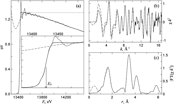
FIG. 1.: Extraction of XAFS from the measured absorption using the smoothing spline. Prior function $p(E)$ for the atomic-like absorption is drawn by dots. Solid lines — $\mu_{0}(E)$, $\chi(k)\cdot k^{2}$, and $\rho(r)$ obtained with use of the prior function; dashed lines — dittos without prior function. The regularizer $\alpha$ is the same for both cases.

First, we address another problem, the well-known spline instability with respect to the small variations of input parameters: number of nodes, nodal values of the processed function, and limits on integral. In our case the spline is most sensitive to $E_{\rm min}$ due to fast growth of $\mu$ in the edge. To raise the stability the method was put forward in viper program which lies in the use of a prior information specifying the shape of $\mu_{0}(E)$ dependence. It is known in advance that the absorption edge without so-called white line constitutes nearly smooth step; the white line, if presents, is added to the step. Denote this prior function as $p(E)$. Now we will tend the second derivative of the sought $\mu_{0}(E)$ not to zero (at the specified deviation of $\mu_{0}$ from $\mu$) but to the second derivative of $p(E)$. The sought $\mu_{0}(E)$ is now minimizes the functional

$$J^{*}(\mu_{0},\mu)=\int^{E_{\rm max}}_{E_{\rm min}}[\mu_{0}^{\prime\prime}(E)-p^{\prime\prime}(E)]^{2}\,dE+\frac{1}{\alpha}\sum^{N+1}_{i=0}[\mu_{0i}-\mu_{i}]^{2}.$$ (3)

As seen, in fact there is no need to know $p(E)$ itself, its second derivative is sufficient. The explicit presence of $p(E)$ in the following formulas should be taken as a consequence of the technical trick applied: at first $p(E)$ is subtracted from the data, then it is added to the found spline.

Represent the second derivatives in finite-difference approximation, introduce $\tilde{\mu}_{0i}=\mu_{0i}-p_{i}$, and denote $\Delta_{i}=E_{i+1}-E_{i}$:

$$J^{*}(\mu_{0},\mu)=\sum^{N}_{i=1}[\tilde{\mu}_{0i-1}\Delta_{i-1}^{-1}-\tilde{\mu}_{0i}(\Delta_{i-1}^{-1}+\Delta_{i}^{-1})+\tilde{\mu}_{0i+1}\Delta_{i}^{-1}]^{2}+\frac{1}{\alpha}\sum^{N+1}_{i=0}[\tilde{\mu}_{0i}-(\mu_{i}-p_{i})]^{2}=J(\tilde{\mu}_{0},\mu_{i}-p_{i}).$$ (4)

Thus, the problem is reduced to the preceding one in which instead of initial data $\mu_{i}$ the difference $\mu_{i}-p_{i}$ is appeared. The sought $\mu_{0}$ is found from the smooth $\tilde{\mu}_{0}$ as $\mu_{0i}=\tilde{\mu}_{0i}+p_{i}$. In Fig. 1 is shown an example of the atomic-like absorption approximation by the smoothing spline with and without the use of prior function. Energy $E_{0}$ was determined at half the step height. Here, we constructed $p(E)$ in the following manner. Found the average value $\bar{\mu}$ of $\mu(E)$ in region $20\leq E\leq 70$ eV above the absorptance maximum. Moving from the beginning of spectrum, assign $p=\mu$ until $\mu>\bar{\mu}$, further $p=\bar{\mu}$. Then $p(E)$ was smoothed 5 times on 3 points. To perform the Fourier transform, $\chi(k)k^{2}$ was brought into the uniform scale with $\delta k=0.03$ Å^-1 and multiplied by a Kaiser-Bessel window with parameter $A=1.5$. As seen, the use of $p(E)$ has led to disappearance of the spurious peak on the absolute value of FT at $r\sim 0.5$ Å.

So far we have considered the atomic-like absorption $\mu_{0}$ to be a smooth function with no peculiarities. However, in some spectra $\mu_{0}$ itself has a fine structure [4, 5] originating from resonance scattering within absorbing atom or from multi-electron transitions. If in these cases, based on theoretical calculations, experimental information, or empirical considerations, one can nearly indicate the location of peculiarities, their width and weight relatively to the step height, then one would readily construct the prior function $p(E)$ and find the correct $\mu_{0}$. Instead of constant value above absorption edge, the prior function would have corresponding valleys and/or peaks.

Let us now define the criterion for determination of smoothing parameter. An attempt to solve the problem was made in Ref. [6], where the requirement was proposed: $H_{R}-H_{N}\geq 0.05H_{M}$, where $H_{R}$ is the average value of the weighted Fourier transform magnitude between 0 and 0.25 Å, $H_{M}$ is the maximum value in the transform magnitude between 1 and 5 Å, $H_{N}$ is the average value of the transform magnitude between 9 and 10 Å attributed to the noise. Obviously, that this criterion cannot pretend to the generality since depends on the weighting (op. cit., $k^{3}$) and the relative contribution of noise and the first coordination shell into spectra.

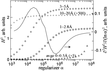
FIG. 2.: The $\rho(r)$ peak heihts squared, $H^{2}$, maximal in the indicated areas and average over the range $0<r<0.5$ Å, as functions of $\alpha$. To the right axis relates the second derivative of the first peak height squared with respect to $\ln\alpha$.

In the program viper we have proposed another approach to the problem based on the consideration of heights of FT peaks as functions of regularizer $\alpha$ (see Fig. 2). On increasing $\alpha$ from zero, $\mu_{0}$ starts to deviate from the experimental absorption $\mu$, $\rho(r)$ is growing and then saturates, the peaks at larger $r$ being saturated earlier. Clearly, that $\alpha$ should be determined by the first peak height since it is the last to saturate. Define the start of saturation on the minimum of second derivative of the first peak squared with respect to $\ln\alpha$. Declare the value of $\alpha$ in the minimum to be optimal. It is seen that the increase of $\alpha$ from the optimal leads to unwanted rapid growth of $\rho$ at low $r$.

In the example in Fig. 1 the regularizer is optimized following our new criterion.

Unfortunately, the method of smoothing spline does not include any approach to the estimations of uncertainties in the $\mu_{0}$ obtained, in contrast to the following two methods.

B Interpolation spline drawn through the varied knots

The method was put forward in Ref. [7]. $N$ knots are equally spaced in $k$ space, through them an interpolation spline is drawn. The ordinates of the knots are varied to minimize $\rho$ or $|\rho-\rho_{\rm st}|$ in the chosen low-$r$ region $0\leq r\leq r_{0}$, where $\rho_{\rm st}$ is the absolute value of the FT of a “standard” $\chi_{\rm st}(k)\cdot k^{w}$, calculated or experimental. The number of knots must not exceed the value $N_{\rm max}=2r_{0}\Delta k/\pi+1$, [8] where $\Delta k$ is the $k$ range of useful data. In the Ref. [7] was asserted that one need to know the “standard” $\chi_{\rm st}(k)\cdot k^{w}$ merely approximately since it used only to get an estimate of the leakage from the first shell to the region minimized. The strange thing is that having omitted the question on the accuracy of found knots (as we show below, rather poor), the authors of the cited work made a fine comparison between several theoretical models for $\chi(k)$ calculations.

In Fig. 1 is shown an example of the method application. Ordinates of the 13 knots ($N_{\rm max}=13.2$) were varied to minimize the difference $\rho-\rho_{\rm st}$ at $0\leq r\leq 1.05$ Å. The function $\chi_{\rm st}(k)$ was calculated using feff6 program [9] (as was pointed above, a crude estimate is sufficient, so details omitted). In the minimized region the $\rho(r)$ is somewhat better than that obtained by the previous method. However, at $k>15$ Å^-1 one can distinguish the obviously wrong behavior of $\chi(k)\cdot k^{2}$, and the first peak on $\rho(r)$ becomes quite distorted.

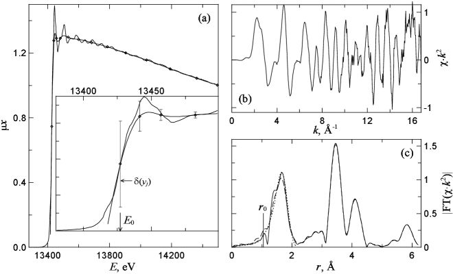
FIG. 3.: Extraction of XAFS from the measured absorption using the interpolation spline through the knots with varied ordinates. On (c) the Fourier transforms are shown for sought $\chi(k)\cdot k^{2}$ (solid), “standard” (dots), and obtained by the previous method (dashed).

Consider now the problem of the accuracy of knot positions $y_{j}$, $j=1,\ldots,N$ in fitting $\rho(r)$ to $\rho_{\rm st}(r)$. As a figure of merit, the $\chi^{2}$-statistics appears:

$$\chi^{2}=\frac{N_{\rm max}}{M}\sum_{m=1}^{M}\frac{[\rho(r_{m})-\rho_{\rm st}(r_{m})]^{2}}{\sigma_{m}^{2}},$$ (5)

where $\sigma_{m}$ are the errors of $\rho(r_{m})$. It can be shown (detailed analysis see in the next article [2]) that under the assumption of uncorrelated knot positions, the mean-square deviation of $y_{j}$ from the obtained through the fit optimal value $\hat{y}_{j}$ equals $\delta(y_{j})=(\frac{1}{2}\partial^{2}\chi^{2}/\partial y_{j}^{2})^{-1/2}$, where the partial derivatives are calculated in the fitting procedure at the minimum. $\sigma_{m}$ are assumed to be constant and equal to the root-mean-square average of $\rho(r)$ between 15 and 25 Å, where solely the noise is present. The errors $\varepsilon_{j}=\delta(y_{j})/[\mu_{0}(E_{j})-\mu_{b}(E_{j})]$ found under such assumptions are shown in Fig. 4 as open circles with the solid line. Notice, that the ussumption that the knot positions are not correlated gives quite optimistic $\varepsilon_{j}$. Actually, several first knot positions appear to be highly correlated; the proper taking into account of the correlations (here we do not present these calculations) raises $\varepsilon_{j}$ at the least as twice. But even these underestimated $\varepsilon_{j}$ are appreciably larger than those given by the following method.

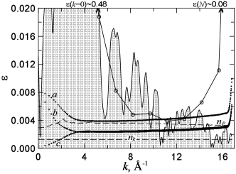
FIG. 4.: Errors of $\chi(k)$ extraction. Solid line with open circles — by the method of interpolation spline drawn through the varied knots. Dots — by the method of bayesian smoothing without ($a$) and with ($b$ $c$) prior information specifying the second derivative. Besides, ($c$) uses additional information that $\mu_{0}(E)$ passes through a point immediately before $E_{0}$. Solid line with filling — the envelope of $\chi(k)$ (not weighted). Dashed lines — the noise estimates from FT ($n_{k}$) and from Poisson counting statistics ($n_{P}$) (see Sec. III).

C Bayesian smooth curve

Ideologically similar to the smoothing spline method is the method of bayesian smoothing (see Appendix on p. Bayesian smoothing and deconvolution) proposed in the program viper. This method also finds the regularized function $\mu_{0}$, the regularizer $\alpha$ is the measure of compromise between smoothness of $\mu_{0}$ and its deviation from $\mu$. In comparison with smoothing spline method, this method has some advantages. (i) Various prior information on $\mu_{0}$ can be considered. (ii) In this method the posterior distributions of all $\mu_{0j}$ are sought for. From those distributions one can find not only average values but also any desirable momenta, which appears to be an additional difficulty for other methods. (iii) In the framework of the method it is possible also to deconvolute $\mu$ with the monochromator rocking curve. The weakness of the method is its low speed (comparing with method II A, not with II B!). On a modern PC the curve drawn through $N\sim 500$ points is smoothed for a few minutes.

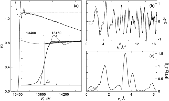
FIG. 5.: Extraction of XAFS from the measured absorption using the bayesian smoothing. Prior function $p(E)$ for the atomic-like absorption is drawn by dots. Solid lines — $\mu_{0}(E)$, $\chi(k)\cdot k^{2}$, and $\rho(r)$ obtained with the use of the prior function; dashed lines — dittos without prior function. The dot line on (c) is obtained without additional requirement for $\mu_{0}(E)$ to pass through a point immediately before $E_{0}$. The regularizer $\alpha$ is the same for all cases and equals to the optimal one found for the smoothing spline.

In Fig. 5 the bayesian smoothing was done on the mesh of 536 experimental points above $E_{0}$, without and with the prior function (its construction is described in Sec. II A). Besides, in the last case another information was used: the atomic-like absorption must coincide with the total absorption (minus pre-edge background) at energies $E<E_{0}$. Therefore, we demanded from the bayesian curve to pass through a point nearest (at left) to $E_{0}$. The values $\bar{\mu}_{0j}$ and $\delta^{2}(\mu_{0j})$ were found by formulas (64) and (67). Since the smoothed values do not lie within the limits of $\pm\delta(\mu_{0j})$ from $\mu_{j}$, we did not look for the most probable smoothness (see. Appendix), instead we considered the regularizer to be known and equal to the optimal one found in the method II A. The introduction of the prior information has significantly diminished the errors of $\chi(k)$ extraction (see dotted curves in Fig. 4) which were defined as $\varepsilon_{j}=\delta(\mu_{0j})/(\bar{\mu}_{0j}-\mu_{bj})$. This is quite natural: any decrease of our ignorance about $\mu_{0}$ should narrow the posterior distribution of $\mu_{0j}$ for all $j$. Of course, this concerns the experimental information as well: errors $\varepsilon_{j}$ are the less the more measured points $N$ the spectrum has. Comparing Fig. 1( ) and Fig. 5(c), it is seen practically perfect coincidence of the results of bayesian smoothing and smoothing spline. From this one can assume the equality of the errors which both methods give.

Could we take into account possible systematic errors in the framework of the method? Yes, if we have the information on their nature and are able to translate it into the mathematics language; such a translation might be rather non-trivial. In any case, now we have the tool to extract from the prior and experimental information not only the sought values but their errors as well.

D Other methods

Consider briefly the methods for $\mu_{0}$ construction not included into the viper program.

A rich variety of computer programs for XAS spectra processing is collected on the International XAFS Society Web-site [10]. The vast majority of them use as an approximation for the atomic-like absorption a smoothing spline or more general piecewise-polynomial representation. For example, in the method of Ref. [11], the construction of $\mu_{0}$ is divided into several stages: $\mu_{0}$ is approximated by a low-degree polynomial, obtained $\chi(k)$ is multiplied by $k^{w}$, additional $\mu_{0}^{\prime}$ is drawn again as a low-degree polynomial and subtracted, a smoothing spline then approximates one more additional $\mu_{0}^{\prime\prime}$. The sum of all $\mu_{0}$’s gives the total atomic-like background. The necessity of the preliminary stages was not discussed op. cit., however, clearly it was caused by the instability of spline with respect to the small variations of input parameters. And the point is not that the preliminary stages make the process stable, but that for each specific spectrum, auxiliary parameters (degrees of polynomials) could provide an acceptable construction of the atomic-like background. Above (in Sec. II A) we proposed the way to rise the stability of spline making the preliminary stages to be redundant.

In Ref. [12] an iterative approach to “atomic background” removal was developed. First a spline is used to obtain a rough estimate of the background; this alone is enough to have a reliable $\chi$ at $k>5-6$ Å^-1. Over that range the $\chi$ obtained is fitted to the theoretical $\chi_{\rm th}$ in $r$-space. The resulting fit parameters are used then to generate $\chi_{\rm th}(k)$ that extends down to low $k$. This function is transformed back into $e$-space and $\mu_{0}$ is obtained as $\mu_{0}=\mu/(\chi_{\rm th}+1)$ that need be a little smoothed or fitted by an additional spline. Since the logic of reasoning was inversed: not “find $\mu_{0}$ to find $\chi$,” but “find $\chi$ to find $\mu_{0}$,” the method is suited for the quest of peculiarities on $\mu_{0}$ curve, not for structural XAFS-researches. Besides, the range of accuracy of the model appears to be unknown in principle: all, that is not described by the model, is included in $\mu_{0}$; the errors of the background approximation are also undefined.

In the old work [13] for the determination of the background absorption $\mu_{0}$ was considered the damping of the XAFS amplitude resulting from the measurements with low resolutions (with a large slit width). The superimposition of two spectra measured with different energy resolutions gives the intersection points, the part of which belong to the $\mu_{0}$. Then through the obtained nodal points a smoothing spline is drawn. As the authors of Ref. [13] noted, the measurements of the spectra with worsened resolution are not necessary; the spectra could be damped by the convolution with a “rocking curve,” approximated by a Gaussian function. Of course, the method is correctly works only with a small variation of the Gaussian curve width since for the large width not only the XAFS amplitude is damped but the very edge is washed out. Because of this only the extended part of a spectrum could be reliably determined.

The damping of the XAFS amplitude can be due to other reasons. For instance, as was pointed in Ref. [13], the nodal points may be obtained from the variable-temperature study. This idea was realized in Ref. [14] and is more sound since the atomic-like background is really independent of temperature and with temperature the XAFS amplitude is changed, not the shape of the edge. But for all that it is important that the phase difference between XAFS of different temperatures was negligible, which is true only for low wave numbers. Unfortunately, the method is suitable only for some particular cases (to say nothing of need for measured temperature series of spectra). Op. cit. it was demonstrated for the x-ray-absorption data for the $L_{3}$ edge of solid Pb. In those spectra the first crossing of $\mu$ and $\mu_{0}$ occurs already at $\sim 15$ eV above edge. In our sample spectra the first crossing occurs only at $\sim 30$ eV, which allows one to find at most 2–3 points and the first of them being situated at $k\gtrsim 2.5$ Å^-1.

An interesting approach to the problem of $\mu_{0}$ determination was reported in Ref. [15]. It is based on the simple identity that relates the FT of some function with the FT of its $n$-th derivative:

$${\rm FT}[f^{(n)}(k)]=(2ir)^{n}{\rm FT}[f(k)],$$ (6)

where the conjugate variables are $k$ and $2r$. Since the atomic-like background is smooth enough, the higher derivatives $\mu^{(n)}(k)$ ($n\geq 2$) are oscillatory near zero. Performing the FT of $\mu^{(n)}(k)\cdot k^{w}$ and using Eq. (6), one obtains the FT of unnormalized would-be $\chi(k)\cdot k^{w}$ (see Fig. 6). Op. cit. the low-$r$ part (which in our example is $0\leq r\lesssim 1.1$) was cut off, and then the back FT was done. As a result, one has the unnormalized $\chi(k)\cdot k^{w}$ and, having subtracted it from the $\mu(k)$, the atomic-like background on which some peculiarities due to multi-electron excitations can be distinguished. Like the method of Ref. [12], this method is suited for the quest of peculiarities on the $\mu_{0}$ curve, not for structural XAFS-researches because of evident distortion of the first peak on the FT by the contribution from the atomic-like background. To illustrate this assertion, in Fig. 6 we show the FT of the second derivative of the $\mu_{0}(k)$ that was found by the present method. As seen, this contribution is not as small.

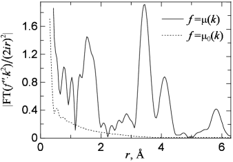
FIG. 6.: On the method of Ref. [15]. Solid curve is the FT of “unnormalized $\chi(k)\cdot k^{2}$”, dotted curve is the contribution from the atomic-like absorption.

If the electronic states of an absorbing atom in gaseous phase and in the compound of interest may be considered as equivalent, $\mu_{0}$ can be set equal to the measured absorption in gas, as was done in Ref [16] for solid, liquid, and gaseous Kr. Some differences in energy positions and relative weights of double-electron excitation channels were taken into account by a model using simple empirical functions which were transferred then to the spectra of liquid and solid Kr. Notice that the proposed in the present paper prior function for the methods of smoothing spline and bayesian smoothing can include additional items corresponding to the multi-electron contributions.

III Errors in $\mu_{0}$ constructing, noise, and choice of limits $k_{\rm min}$ $k_{\rm max}$

For what we need to know the errors of XAFS-function extraction? First, without knowing of these values one cannot in principle aim at their minimization. Second, they are used in the definition of $\chi^{2}$-statistics in the fitting problems; their underestimation is a source of unjustified optimistic errors of fitting parameters. Third, along with analysis of the noise, the errors of $\mu_{0}$ construction allow us to choose the limits of reliable EXAFS signal, $k_{\rm min}$ and $k_{\rm max}$.

Unfortunately, the issue of quality of XAFS extraction from the measured absorption has not been addressed properly. We see several reasons for that. On the one hand, not having a correctly developed approach to the estimation of the errors of final results (interatomic distances, Debye-Waller factors etc. found via fitting), the errors of EXAFS extraction are useful. On the other hand, only a few methods include approaches to their estimations.

Easily one can compare the errors of different methods (see Fig. 4) and then choose the most reliable one. The problem of plausible limitations on the absolute value of the errors is more difficult. Define “signal” as the envelope of $\chi(k)$ (solid line with gray filling in Fig. 4). It is quite reasonable to demand that the errors of $\mu_{0}$ construction were less than XAFS signal. For the method of the interpolation spline drawn through the varied knots to meet this requirement leads to the restriction on the photoelectron wave numbers: $2\lesssim k\lesssim 14$ Å^-1. For the bayesian curve $a$ this range is $0\leq k\lesssim 14$ Å^-1, for the bayesian curves $b$ and $c$ this range is wider: $0\leq k\lesssim 16$ Å^-1.

Another factor that limitates the spectrum length is the presence of noise. To determine the noise is a straightforward task for $r$-space, where XAFS signals at high $r$ have clearly noise character. By Parseval’s identity the noise in $r$-space is related with the noise in $k$-space [17]:

$$\int_{k_{\rm min}}^{k_{\rm max}}|n_{k}k^{w}|^{2}dk=2\int_{0}^{\pi/2dk}|n_{r}|^{2}dr.$$ (7)

Substitute the mean value over the range $15<r<25$ Å of the FT magnitude squared for $|n_{r}|^{2}$. Then

$$n_{k}^{2}=\langle|n_{r}^{2}|\rangle\frac{\pi}{dk}\ \frac{2w+1}{k_{\rm max}^{2w+1}-k_{\rm min}^{2w+1}}.$$ (8)

As seen from the formula, $n_{k}$ depends on $dk$, the size of evenly-spaced $k$-grid. Although above we already have used the Fourier transform, the question of choice of $dk$ was not raised yet. The algorithm of fast FT needs the transformed function to be set on a uniform grid. Having chosen a small $dk$, we artificially obtain the large number of “experimental” values. Naturally, this trick would not give more information than we have, and the errors $n_{k}$ must be large at the small $dk$. In our example the choice of $dk$ (0.03 Å^-1) was based on the equality of numbers of experimental points and the nodes of the grid. The signal-to-noise ratio obtained is greater than unity for all the spectrum (see Fig. 4). There was no doubt in that: the signal is visually distinguished even for the very extended end of the spectrum (see Fig. 1(b) and Fig. 5(b)).

The noise can be estimated based on the bayesian considerations [18]. Let after measurements we have the values of counts from the solid-state or gas-filled detectors and let there is a positive real number $\lambda$ such that the probability that a single count occurs in the time interval $dt$ is

$$P(1|\lambda)=\lambda dt.$$ (9)

It can be shown [19] that merely from this assumption follows that the counts obey the Poisson distribution law:

$$P(N|\lambda,T)=\frac{(\lambda T)^{N}\exp(-\lambda T)}{N!},$$ (10)

where $T$ is the sampling time. The problem is to find the intensity $\lambda$ and its variance. Using Bayes theorem and introducing prior probabilities $P(N)=1/N$ and $P(\lambda)=1/\lambda$ [20], one obtains:

$$P(\lambda|N,T)=\frac{P(N|\lambda,T)P(\lambda)}{P(N)}=\frac{T(\lambda T)^{N-1}\exp(-\lambda T)}{(N-1)!},$$ (11)

that is after measurement the variate $2T\lambda$ follows the $\chi^{2}$-distribution with $2N$ degrees of freedom. It is easy to find that $\bar{\lambda}=N/T$, $\overline{\lambda^{2}}=N(N+1)/T^{2}$, and the variance of intensity is $\delta\lambda=\sqrt{N}/T$.

Denote counts from detectors measuring $i_{0}$ and $i_{1}$ as $I_{0}$ and $I_{1}$. By definition the variate $\xi=\frac{i_{0}/2I_{0}}{i_{1}/2I_{1}}$ follows Fisher’s $F$-distribution with $(2I_{0},2I_{1})$ degrees of freedom. Its expected value and variance are known: $\bar{\xi}=I_{1}/(I_{1}-1)$, $\delta^{2}\xi=I_{1}^{2}(I_{0}+I_{1}-1)/((I_{1}-1)^{2}(I_{1}-2)I_{0})$, from where we find for the absorption in the fluorescence mode ($\mu x=i_{0}/i_{1}$):

$$\overline{i_{0}/i_{1}}=\frac{I_{0}}{I_{1}-1},\qquad\delta^{2}(i_{0}/i_{1})=\frac{I_{0}(I_{0}+I_{1}-1)}{(I_{1}-1)^{2}(I_{1}-2)}.$$ (12)

Further, the variate $\eta=\frac{1}{2}\ln\xi$ follows $z$-distribution (Fisher’s distribution of variance ratio) with $(2I_{0},2I_{1})$ degrees of freedom. Its expected value and variance are known: $\bar{\eta}=0$, $\delta^{2}\eta=\frac{1}{4}(I_{1}+I_{1})/(I_{0}I_{1})$, from where we find for the absorption in the transmission mode ($\mu x=\ln(i_{0}/i_{1})$):

$$\overline{\ln(i_{0}/i_{1})}=\ln\frac{I_{0}}{I_{1}},\qquad\delta^{2}\ln(i_{0}/i_{1})=\frac{1}{I_{0}}+\frac{1}{I_{1}}.$$ (13)

The noise of XAFS-function is

$$n_{P}=\frac{\delta\mu}{\mu_{0}-\mu_{b}}=\left(\frac{1}{I_{0}}+\frac{1}{I_{1}}\right)^{1/2}\frac{1}{\mu_{0}-\mu_{b}}.$$ (14)

In our example this noise at $k\gtrsim 15$ Å^-1 becomes greater than signal (see Fig. 4). What is the reason for such significant difference between the really present noise $n_{k}$ and its statistical estimate $n_{P}$? Of course, the reason is in the false premise (9). In practice this condition is realized as: $P(c|\lambda)=\lambda dt$. For example, the photocurrent in an ion-chamber depends on gas pressure, potential applied etc.; these dependencies are contained in $c$. In other words, the amplification path works in such a way that one photon gives birth to $c$ counts. There is no difficulty in writing the posterior distribution for the generalized premise:

$$P(\lambda|N,T)=\frac{T(\lambda T)^{\frac{N}{c}-1}\exp(-\lambda T)}{\Gamma(N/c)},$$ (15)

with $\bar{\lambda}=N/(cT)$ and $\delta\lambda=\sqrt{N/c\phantom{\,}}/T$. Thus, having unknown $c$ (and implicitly assigning $c=1$), we got wrong variances for $i_{0}/i_{1}$ and $\ln(i_{0}/i_{1})$. Unfortunately, in the most of real experiments the association between the probability of a single count event and the radiation intensity (via $c$) is unknown. In spite of this, the Poisson counting statistics is traditionally used for a long time. For example, in Ref. [21] signal-to-noise ratios are evaluated (assuming $c=1$) for the different detection schemes.

Practically all programs for XAFS spectra processing [10] to estimate the noise use the Fourier analysis. But then it is the noise that they use as uncertainties $\varepsilon_{i}$ of $\chi(k)$ determination in definition of $\chi^{2}$-statistics:

$$\chi^{2}=\frac{N_{\rm max}}{M}\sum_{i=1}^{M}\frac{[(\chi_{\rm exp})_{i}-(\chi_{\rm mod})_{i}]^{2}}{\varepsilon_{i}^{2}}.$$ (16)

It would be more correct to consider as $\varepsilon_{i}$ the larger from the two: the noise and the errors of the construction of $\mu_{0}$. In our case (and as a rule) the latter are essentially greater (especially in the method II B) than the noise. In the following paper [2] we shall show how the understated $\varepsilon_{i}$ lead to optimistic errors of structural parameters.

IV XAFS-function correction

Because of one reason or another the experimental XAFS might be distorted. Consider some of them.

(i) Let the counts ($I$) from detectors are associated with the intensities ($i$) as $i_{0}=\varkappa_{0}I_{0}$ and $i_{1}=\varkappa_{1}I_{1}$. Then the absorption (in the transmission mode) equals:

$$\mu x=\ln(i_{0}/i_{1})=\ln(I_{0}/I_{1})+\ln(\varkappa_{0}/\varkappa_{1}).$$ (17)

The second term is a slightly varied function of energy and can be taken into account in independent experiments. Such a distortion appears, for instance, if the absorptance of the gas in ion-chamber detectors depends on energy.

(ii) If some part of incident radiation is not attenuated in the sample as much as expected (due to the pinholes in the sample, harmonics in the incoming beam etc.), that is $i_{0}=\varkappa_{0}I_{0}+b$, then the real absorption is connected with the measured $I_{0}$ and $I_{1}$ in a complicated way. In Ref. [22] the possible decrease of XAFS amplitude shown to be essential even at low $b/(\varkappa_{0}I_{0})$ but thick samples. At known ratio $b/(\varkappa_{0}I_{0})$, the correcting factor can be easily obtained.

(iii) In the fluorescence mode, due to absorptance of the fluorescent signal in the sample itself XAFS spectra strongly depend on the detection geometry. In Ref. [23] the correcting functions are found explicitly.

(iv) The problem of glitches is widespread in the XAFS analysis. The glitches are due to multiple Bragg reflection being satisfied simultaneously and for each given monochromator are manifested in the strictly determined spectral positions. In most cases the glitches seen on curves $I_{0}(E)$ and $I_{1}(E)$, vanish on $I_{0}/I_{1}$ ratio. If not, one can easily get rid of them. For instance, the glitch area, usually extremely thin, is smoothed or, with fixed ends, replaced by a straight-line segment. The main thing in the correct analysis of glitches is their detection.

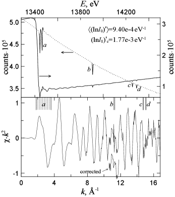
FIG. 7.: Energy dependence of experimental counts from ion-chambers. Curve $I_{0}(E)$ relates to the left axis, $I_{1}(E)$ — to the right one. In glitch areas the absolute value of the derivative is greater than the critical level specified. On $\chi(k)\cdot k^{2}$ only the glitch $b$ is manifested. The displaced fragment is $\chi(k)\cdot k^{2}$ after correction.

To detect a glitch on curves $\mu$ or $\chi k^{w}$ is practically impossible. For this, one needs the primary data $I_{0}(E)$ and $I_{1}(E)$, not $\ln(I_{0}/I_{1})$ nor $I_{0}/I_{1}$. Out of glitches the intensity of incident radiation smoothly, ignoring the noise, depends on energy (see Fig. 7). The idea of detection of glitches via critical level for the derivative $|d\ln I_{0}/dE|_{c}$ is self-evident. For the presented in Fig. 7 $I_{0}(E)$ curve the absolute value of the derivative in the glitch areas is greater than the critical value chosen to be equal to $1.77\cdot 10^{-3}$  ^-1. Having extracted the XAFS, one can see that the first (paired) glitch $a$ is not manifested on $\chi(k)\cdot k^{2}$, the last two ($c$ $d$) are obscured by the noise, solely glitch $b$ is clearly pronounced. Now, being in the firm belief that this is not a part of the XAFS, one can eliminate the glitch with ease. Here, we fixed its ends on $\mu(E)$, replaced it by the straight-line segment, and constructed $\chi(k)\cdot k^{2}$ again.

V Conclusion

In this paper we have considered all stages of XAFS function extraction from the measured absorption. We focused our attention on the most important stage, construction of the atomic-like absorption $\mu_{0}$.

For the wide-spread method of approximation of $\mu_{0}$ by a smoothing spline we have proposed the way to raise the stability by including the prior information about absorption edge shape (“nearly step” or “nearly step with a white line”). Besides we have propose a new reliable criterion for determination of the smoothing regularizer.

A new method for approximation of $\mu_{0}$ is proposed, the method of bayesian smoothing. It can include various prior information, which raises the accuracy of XAFS determination. Following this method one finds the distributions of $\mu_{0}$ in each experimental point, from which one can find not only average values but also any desirable momenta, which appears to be an additional difficulty for other methods. This method was shown to give more accurate atomic-like background than that obtained by the method of Ref [7].

Particular attention has been given to the analysis of noise. We have discussed the difficulties of its estimates on the basis of statistical approach. More reliable is the determination of noise from the Fourier transform. We have shown that the experimental noise is essentially less than the errors of $\mu_{0}$ construction, and the use of values of noise in the $\chi^{2}$-statistics definition appears to be erroneous since leads to the unjustified optimistic errors of structural parameters inferred in fitting procedures. For detailed consideration of the accuracy of fitting parameters see the following paper [2].

Bayesian smoothing and deconvolution

1 Posterior distribution for smoothed data

Consider general linear problem of data smoothing with the use of statistical methods (for introduction see review by Turchin et al. [24] and the articles from Web-site bayes.wustl.edu). Let data $\bf d$ are defined on the mesh $x_{1},\ldots,x_{N}$ and consist of the true values $\bf t$ and the additive noise $\bf n$:

$$d_{i}=t_{i}+n_{i},\qquad i=1,\ldots,N.$$ (18)

The problem of smoothing is to find the best estimates of $\bf t$. For an arbitrary node $j$, find the probability density function for $t_{j}$ given the data $\bf d$:

$$P(t_{j}|{\bf d})=\int\cdots dt_{i\neq j}\cdots P({\bf t}|{\bf d}),$$ (19)

where $P({\bf t}|{\bf d})$ is the joint probability density function for all values $\bf t$, and the integration is done over all $t_{i\neq j}$. According to Bayes theorem,

$$P({\bf t}|{\bf d})=\frac{P({\bf d}|{\bf t})P({\bf t})}{P({\bf d})},$$ (20)

$P({\bf t})$ being the joint prior probability for all $t_{i}$, $P({\bf d})$ is a normalization constant. Assuming that the values $n_{i}$ are independent in different nodes and normally distributed with zero expected values, the probability $P({\bf d}|{\bf t})$, so-called likelihood function, is given by

$$P({\bf d}|{\bf t},\sigma)=(2\pi\sigma^{2})^{-N/2}\exp\Bigl{(}-\frac{1}{2\sigma^{2}}\sum_{k=1}^{N}(d_{k}-t_{k})^{2}\Bigr{)},$$ (21)

where the standard deviation of the noise, $\sigma$, appears as a known value. Later, we apply the rules of probability theory to remove $\sigma$ from the problem.

Now define prior probability $P({\bf t})$. Let we know in advance that the function $t(x)$ is smooth enough. To specify this information, introduce the norm of the second derivative and indicate its expected approximate value:

$$\Omega(t(x))=\int\left(\frac{d^{2}t}{dx^{2}}\right)^{2}\,dx\approx\omega.$$ (22)

Denote $\Delta_{i}=x_{i+1}-x_{i}$, $i=1,\ldots,N-1$ and represent the second derivative in the finit-difference form:

$$\Omega(t(x))\equiv\Omega({\bf t})=\sum^{N-1}_{i=2}[t_{i-1}\Delta_{i-1}^{-1}-t_{i}(\Delta_{i-1}^{-1}+\Delta_{i}^{-1})+t_{i+1}\Delta_{i}^{-1}]^{2}\equiv\sum^{N}_{k,l=1}\Omega_{kl}t_{k}t_{l}.$$ (23)

$\Omega_{kl}$ is a five-diagonal symmetric matrix with the following non-zero elements:

$$\Omega_{11} = \Delta_{1}^{-1}\Delta_{2}^{-2},\quad\Omega_{22}=\Delta_{2}^{-1}(\Delta_{1}^{-1}+\Delta_{2}^{-1})^{2}+\Delta_{2}^{-2}\Delta_{3}^{-1},\quad\Omega_{12}=-(\Delta_{1}\Delta_{2})^{-1}(\Delta_{1}^{-1}+\Delta_{2}^{-1}),$$ (25)

$$\cdots\cdots\cdots\cdots$$

$$\Omega_{ii} = \Delta_{i}^{-1}(\Delta_{i}^{-1}+\Delta_{i-1}^{-1})^{2}+\Delta_{i}^{-2}\Delta_{i+1}^{-1}+\Delta_{i-1}^{-3},$$ (26)

$$\Omega_{i-1,i} = -\Delta_{i-1}^{-2}(\Delta_{i-1}^{-1}+\Delta_{i-2}^{-1})-(\Delta_{i-1}\Delta_{i})^{-1}(\Delta_{i-1}^{-1}+\Delta_{i}^{-1}),$$ (27)

$$\Omega_{i-2,i} = \Delta_{i-2}^{-1}\Delta_{i-1}^{-2},$$ (29)

$$\cdots\cdots\cdots\cdots$$

$$\Omega_{NN} = \Delta_{N-1}^{-3},\quad\Omega_{N-1,N-1}=\Delta_{N-1}^{-1}(\Delta_{N-1}^{-1}+\Delta_{N-2}^{-1})^{2}+\Delta_{N-2}^{-3},\quad\Omega_{N-1,N}=-\Delta_{N-1}^{-2}(\Delta_{N-1}^{-1}+\Delta_{N-2}^{-1}).$$ (30)

In order to introduce the minimum information in addition to that contained in (23), from all normalized to unity functions $P({\bf t})$ which satisfy the condition (23) we choose a single one that contains minimum information about t that is minimizes the functional

$$I[P({\bf t})]=\int P({\bf t})\ln P({\bf t})\,d{\bf t}+\beta\Bigl{[}1-\int P({\bf t})\,d{\bf t}\Bigr{]}+\gamma\Bigl{[}\omega-\int\Omega({\bf t})\,P({\bf t})\,d{\bf t}\Bigr{]},$$ (31)

where $\beta$ and $\gamma$ are the Larrange multipliers. In minimizing $I[P({\bf t})]$, one obtains the equation set

$$\ln P({\bf t})+1-\beta-\gamma\Omega({\bf t}) = 0$$ (32)

$$\int P({\bf t})\,d{\bf t} = 1$$ (33)

$$\int\Omega({\bf t})\,P({\bf t})\,d{\bf t} = \omega,$$ (34)

that has a solution:

$$P({\bf t})=(\lambda_{1}\cdots\lambda_{N})^{-1/2}\Bigl{(}\frac{2\pi\sigma^{2}}{\alpha}\Bigr{)}^{-N/2}\exp\Bigl{(}-\frac{\alpha}{2\sigma^{2}}\Omega({\bf t})\Bigr{)},$$ (35)

where $\alpha/2\sigma^{2}=\gamma=N/2\omega$, and $\lambda_{1},\ldots,\lambda_{N}$ are the eigenvalues of the matrix $\Omega_{kl}$. The regularizer $\alpha$ will be used to control the smoothness of ${\bf t}$. The prior distribution obtained is a “soft” one, that is does not demand from the solution to have a strictly prescribed form.

Thus, we have for the probability density function:

$$P(t_{j}|{\bf d},\sigma,\alpha) \propto \int\cdots dt_{i\neq j}\cdots\sigma^{-2N}\alpha^{N/2}\exp\Bigl{(}-\frac{\alpha}{2\sigma^{2}}\sum^{N}_{k,l=1}\Omega_{kl}t_{k}t_{l}\Bigr{)}\exp\Bigl{(}-\frac{1}{2\sigma^{2}}\sum_{k=1}^{N}(d_{k}-t_{k})^{2}\Bigr{)}$$ (36)

$$= \int\cdots dt_{i\neq j}\cdots\sigma^{-2N}\alpha^{N/2}\exp\Bigl{(}-\frac{1}{2\sigma^{2}}\bigl{[}{\bf d}^{2}-2\sum^{N}_{k=1}d_{k}t_{k}+\sum_{k,l=1}^{N}g_{kl}t_{k}t_{l}\bigr{]}\Bigr{)},$$ (37)

where

$$g_{kl}=\alpha\Omega_{kl}+\delta_{kl},\qquad{\bf d}^{2}=\sum_{k=1}^{N}d_{k}^{2}.$$ (38)

Since there is no integral over $t_{j}$, separate it from the other integration variables:

$$P(t_{j}|{\bf d},\sigma,\alpha) \propto \sigma^{-2N}\alpha^{N/2}\exp\Bigl{(}-\frac{1}{2\sigma^{2}}[{\bf d}^{2}-2d_{j}t_{j}+g_{jj}t_{j}^{2}]\Bigr{)}$$ (40)

$$\times\int\cdots dt_{i\neq j}\cdots\exp\Bigl{(}-\frac{1}{2\sigma^{2}}\bigl{[}\mathop{{\sum}\smash{{}^{j}}}_{k,l=1}^{N}g_{kl}t_{k}t_{l}-2\mathop{{\sum}\smash{{}^{j}}}_{k=1}^{N}[d_{k}-g_{kj}t_{j}]t_{k}\bigr{]}\Bigr{)},$$

Here, the symbol $j$ near the summation signs denotes the absence of $j$-th item. Further, find the eigenvalues $\lambda^{\prime}_{i}$ and corresponding eigenvectors ${\bf e}_{i}$ of the matrix $g_{kl}$ in which the $j$-th row and column are deleted, and change the variables:

$$b_{i}=\sqrt{\lambda^{\prime}_{i}}\mathop{{\sum}\smash{{}^{j}}}_{k=1}^{N}t_{k}e_{ik},\qquad t_{k}=\mathop{{\sum}\smash{{}^{j}}}_{i=1}^{N}\frac{b_{i}e_{ik}}{\sqrt{\lambda^{\prime}_{i}}}\qquad(i,k\neq j).$$ (41)

Using the properties of eigenvectors:

$$\mathop{{\sum}\smash{{}^{j}}}_{k=1}^{N}g_{lk}e_{ik}=\lambda^{\prime}_{i}e_{il},\qquad\mathop{{\sum}\smash{{}^{j}}}_{k=1}^{N}e_{lk}e_{ik}=\delta_{li}\qquad(l,i\neq j),$$ (42)

one obtains:

$$P(t_{j}|{\bf d},\sigma,\alpha) \propto \sigma^{-2N}\alpha^{N/2}\exp\Bigl{(}-\frac{1}{2\sigma^{2}}[({\bf d}^{2}-{\bf h}^{2})-2t_{j}(d_{j}-{\bf h}{\bf u})+t_{j}^{2}(g_{jj}-{\bf u}^{2})]\Bigr{)}$$ (44)

$$\times\int\cdots db_{l\neq j}\cdots\exp\Bigl{(}-\frac{1}{2\sigma^{2}}\mathop{{\sum}\smash{{}^{j}}}_{i=1}^{N}[b_{i}-h_{i}+u_{i}t_{j}]^{2}\Bigr{)},$$

where new quantities were introduced:

$$h_{i}=\frac{1}{\sqrt{\lambda^{\prime}_{i}}}\mathop{{\sum}\smash{{}^{j}}}_{k=1}^{N}d_{k}e_{ik},\qquad u_{i}=\frac{1}{\sqrt{\lambda^{\prime}_{i}}}\mathop{{\sum}\smash{{}^{j}}}_{k=1}^{N}g_{kj}e_{ik},\qquad$$ (45)

$${\bf h}^{2}=\mathop{{\sum}\smash{{}^{j}}}_{i=1}^{N}h_{i}^{2},\qquad{\bf u}^{2}=\mathop{{\sum}\smash{{}^{j}}}_{i=1}^{N}u_{i}^{2},\qquad{\bf h}{\bf u}=\mathop{{\sum}\smash{{}^{j}}}_{i=1}^{N}h_{i}u_{i}.$$ (46)

Evaluating the $N-1$ integrals in (44), one finally obtains the posterior probability for $j$-th node:

$$P(t_{j}|{\bf d},\sigma,\alpha)\propto\sigma^{-(N+1)}\alpha^{N/2}\exp\Bigl{(}-\frac{1}{2\sigma^{2}}[({\bf d}^{2}-{\bf h}^{2})-2t_{j}(d_{j}-{\bf h}{\bf u})+t_{j}^{2}(g_{jj}-{\bf u}^{2})]\Bigr{)}.$$ (47)

2 Eliminating nuisance parameters

In most real problems $\sigma$ and $\alpha$ are not known. To eliminate $\sigma$ is a quite straightforward problem:

$$P(t_{j}|{\bf d},\alpha)=\int d\sigma P(t_{j},\sigma|{\bf d},\alpha)=\int d\sigma P(\sigma)P(t_{j}|{\bf d},\sigma,\alpha),$$ (48)

one needs only to know a prior probability $P(\sigma)$. Having no specific information about $\sigma$, a Jeffreys prior $P(\sigma)=1/\sigma$ is assigned [20]. Then

$$P(t_{j}|{\bf d},\alpha) \propto \int_{0}^{\infty}d\sigma\sigma^{-(N+2)}\exp\Bigl{(}-\frac{1}{2\sigma^{2}}[({\bf d}^{2}-{\bf h}^{2})-2t_{j}(d_{j}-{\bf h}{\bf u})+t_{j}^{2}(g_{jj}-{\bf u}^{2})]\Bigr{)}$$ (49)

$$\propto [({\bf d}^{2}-{\bf h}^{2})-2t_{j}(d_{j}-{\bf h}{\bf u})+t_{j}^{2}(g_{jj}-{\bf u}^{2})]^{-(N+1)/2}.$$ (50)

Introducing the substitution

$$w_{j}^{2}=N\frac{(g_{jj}-{\bf u}^{2})^{2}}{({\bf d}^{2}-{\bf h}^{2})(g_{jj}-{\bf u}^{2})-(d_{j}-{\bf h}{\bf u})^{2}}\left(t_{j}-\frac{d_{j}-{\bf h}{\bf u}}{g_{jj}-{\bf u}^{2}}\right)^{2},$$ (51)

one obtains the Student $t$-distribution with $N$ degrees of freedom:

$$P(w_{j}|{\bf d},\alpha)\propto\Bigl{(}1+\frac{w_{j}^{2}}{N}\Bigr{)}^{-(N+1)/2}$$ (52)

with zero average and the variance $N/(N-2)$. From where one finds for $t_{j}$:

$$\bar{t}_{j}=\frac{d_{j}-{\bf h}{\bf u}}{g_{jj}-{\bf u}^{2}},\qquad\ \delta^{2}(t_{j})=\frac{({\bf d}^{2}-{\bf h}^{2})(g_{jj}-{\bf u}^{2})-(d_{j}-{\bf h}{\bf u})^{2}}{(g_{jj}-{\bf u}^{2})^{2}}\frac{1}{N-2}.$$ (53)

Thus, we have got rid of unknown $\sigma$ and found the expressions for mean values $t_{j}$ and their dispersions at known regularizer $\alpha$. To eliminate the latter is more difficult. The idea is not to find the smoothest solution, but the solution of the most probable smoothness. For that we will find the posterior probability:

$$P(\alpha|{\bf d})=\int d{\bf t}d\sigma P(\alpha,\sigma,{\bf t}|{\bf d})=\int d{\bf t}d\sigma P(\alpha,\sigma)P({\bf t}|\alpha,\sigma,{\bf d}).$$ (54)

Assuming that $\alpha$ and $\sigma$ are independent and using Bayes theorem (20), one obtains:

$$P(\alpha|{\bf d})\propto\int d{\bf t}d\sigma P(\alpha)P(\sigma)P({\bf t}|\alpha,\sigma)P({\bf d}|{\bf t},\alpha,\sigma).$$ (55)

Substituting (35) for the prior probability $P({\bf t}|\alpha,\sigma)$, (21) for the likelihood, and a Jeffreys prior $P(\sigma)=1/\sigma$ and $P(\alpha)=1/\alpha$, one obtains the posterior distribution for the regularizer $\alpha$:

$$P(\alpha|{\bf d}) \propto \int d{\bf t}d\sigma\sigma^{-2N-1}\alpha^{N/2-1}\exp\Bigl{(}-\frac{\alpha}{2\sigma^{2}}\sum^{N}_{k,l=1}\Omega_{kl}t_{k}t_{l}\Bigr{)}\exp\Bigl{(}-\frac{1}{2\sigma^{2}}\sum_{k=1}^{N}(d_{k}-t_{k})^{2}\Bigr{)}$$ (56)

$$= \int d{\bf t}d\sigma\sigma^{-2N-1}\alpha^{N/2-1}\exp\Bigl{(}-\frac{1}{2\sigma^{2}}\bigl{[}{\bf d}^{2}-2\sum^{N}_{k=1}d_{k}t_{k}+\sum_{k,l=1}^{N}g_{kl}t_{k}t_{l}\bigr{]}\Bigr{)},$$ (57)

where matrix $g_{kl}$ was defined in (38). After its diagonalization, analogously to what was done above, finally one obtains:

$$P(\alpha|{\bf d})\propto(\lambda^{\prime}_{1}\cdots\lambda^{\prime}_{N})^{-1/2}\alpha^{N/2-1}[{\bf d}^{2}-{\bf h}^{2}]^{-N/2},$$ (58)

where ${\bf h}^{2}$ is given by

$${\bf h}^{2}=\sum_{i=1}^{N}h_{i}^{2},\qquad h_{i}=\frac{1}{\sqrt{\lambda^{\prime}_{i}}}\sum_{k=1}^{N}d_{k}e_{ik},$$ (59)

and $\lambda^{\prime}_{i}$ and ${\bf e}_{i}$ are the eigenvalues and eigenvectors of $g_{kl}$. Having found the maximum of the posterior probability (58) or having averaged over it the expression (53), one has the sought ${\bf t}$ with the most probable smoothness. However it is necessary to point out that this procedure narrows the applicability of the bayesian smoothing down to the class of tasks where the smoothed values lie in most within the limits $\pm\sigma$ from the most probable. In practice, there possible other tasks where the condition (18) is treated more wider and the smoothed values exceed the bounds of noise.

3 Expressions for smoothed values and their variances

The formulas (53) appear useless in practice since require to find the eigenvalues and eigenvectors for the matrix of rank $N-1$ on each node. Those formulas have merely a methodological value: the explicit expressions for posterior probabilities enable one to find the average of arbitrary function of $t_{j}$. However, $\bar{t}_{j}$ and $\delta^{2}(t_{j})$ could be found significantly easier. Using (48) and (36), represent $\bar{t}_{j}$ as:

$$P(\sigma)P(t_{j}|{\bf d},\sigma,\alpha)dt_{j}$$ (60)

$$\propto \int d{\bf t}d\sigma\sigma^{-2N-1}t_{j}\exp\Bigl{(}-\frac{1}{2\sigma^{2}}\bigl{[}{\bf d}^{2}-2\sum^{N}_{k=1}d_{k}t_{k}+\sum_{k,l=1}^{N}g_{kl}t_{k}t_{l}\bigr{]}\Bigr{)}.$$ (61)

Performing the diagonalization, one obtains:

$$\bar{t}_{j} \propto \int d{\bf b}d\sigma\sigma^{-2N-1}\exp\Bigl{(}-\frac{1}{2\sigma^{2}}[{\bf d}^{2}-{\bf h}^{2}]\Bigr{)}\Bigl{(}\sum_{i=1}^{N}\frac{b_{i}e_{ij}}{\sqrt{\lambda^{\prime}_{i}}}\Bigr{)}\exp\Bigl{(}-\frac{1}{2\sigma^{2}}\sum_{i=1}^{N}[b_{i}-h_{i}]^{2}\Bigr{)}$$ (62)

$$\propto \sum_{i=1}^{N}\frac{h_{i}e_{ij}}{\sqrt{\lambda^{\prime}_{i}}}\int d\sigma\sigma^{-N-1}\exp\Bigl{(}-\frac{1}{2\sigma^{2}}[{\bf d}^{2}-{\bf h}^{2}]\Bigr{)},$$ (63)

from where

$$\bar{t}_{j}=\sum_{i=1}^{N}\frac{h_{i}e_{ij}}{\sqrt{\lambda^{\prime}_{i}}}.$$ (64)

Analogously, for the variance $\delta(t_{j})$ one has:

$$\delta^{2}(t_{j}) \propto \int d{\bf b}d\sigma\sigma^{-2N-1}\exp\Bigl{(}-\frac{1}{2\sigma^{2}}[{\bf d}^{2}-{\bf h}^{2}]\Bigr{)}\Bigl{(}\sum_{i=1}^{N}\frac{(b_{i}-h_{i})e_{ij}}{\sqrt{\lambda^{\prime}_{i}}}\Bigr{)}^{2}\exp\Bigl{(}-\frac{1}{2\sigma^{2}}\sum_{i=1}^{N}[b_{i}-h_{i}]^{2}\Bigr{)}$$ (65)

$$\propto \sum_{i=1}^{N}\frac{e_{ij}^{2}}{\lambda^{\prime}_{i}}\int d\sigma\sigma^{-N-1}\exp\Bigl{(}-\frac{1}{2\sigma^{2}}[{\bf d}^{2}-{\bf h}^{2}]\Bigr{)}\sigma^{2}.$$ (66)

Normalizing, one finally obtains:

$$\delta^{2}(t_{j}) = \frac{\int d\sigma\sigma^{-N+1}\exp\left(-[{\bf d}^{2}-{\bf h}^{2}]/2\sigma^{2}\right)}{\int d\sigma\sigma^{-N-1}\exp\left(-[{\bf d}^{2}-{\bf h}^{2}]/2\sigma^{2}\right)}\sum_{i=1}^{N}\frac{e_{ij}^{2}}{\lambda^{\prime}_{i}}$$ (67)

$$= \ \frac{\Gamma\!\left(\frac{N}{2}-1\right)}{\left([{\bf d}^{2}-{\bf h}^{2}]/2\right)^{N/2-1}}\ \frac{\left([{\bf d}^{2}-{\bf h}^{2}]/2\right)^{N/2}}{\Gamma\!\left(\frac{N}{2}\right)}\sum_{i=1}^{N}\frac{e_{ij}^{2}}{\lambda^{\prime}_{i}}=\frac{[{\bf d}^{2}-{\bf h}^{2}]}{N-2}\sum_{i=1}^{N}\frac{e_{ij}^{2}}{\lambda^{\prime}_{i}}.$$ (68)

Now we got the usable formulas, which require to find the eigenvalues and eigenvectors for the matrix of rank $N$ just one time.

4 Addenda to the bayesian smoothing

(i) Let the curvature of the function $t(x)$ is approximately known in advance. To specify this information, introduce the norm of the difference between $d^{2}t/dx^{2}$ and approximately known second derivative $d^{2}\!f/dx^{2}$:

$$\Omega(t(x))=\int\left(\frac{d^{2}t}{dx^{2}}-\frac{d^{2}\!f}{dx^{2}}\right)^{2}\,dx\approx\omega.$$ (69)

Notice, that there is no need to know $f(x)$ itself, its second derivative is sufficient. The explicit presence of $f(x)$ in the following formulas should be taken as a consequence of the technical trick applied: at first $f(x)$ is subtracted from the data, then it is added to the found solution.

Everywhere in formulas (23–67) make the substitutions:

$$\tilde{t}_{i}=t_{i}-f_{i},\qquad\tilde{d}_{i}=d_{i}-f_{i},\qquad i=1,\ldots,N.$$ (70)

Performing the described above procedure for smoothing, one finds $\tilde{t}_{i}$, from which by inverse transformation the sought vector is given by ${\bf t}=\tilde{{\bf t}}+{\bf f}$.

(ii) In some tasks the value on the starting (zero) node is known without measurement. This sort of prior information represents a “hard” one, that is it restricted the class of possible solutions; in the given case the solution must pass through the known zero node. The quadratic form $\Omega({\bf t})$ (or $\Omega(\tilde{{\bf t}})$ in the case of approximately known second derivative) in the expression for the prior probability has changed:

$$\Omega({\bf t})=\sum^{N-1}_{i=1}[t_{i-1}\Delta_{i-1}^{-1}-t_{i}(\Delta_{i-1}^{-1}+\Delta_{i}^{-1})+t_{i+1}\Delta_{i}^{-1}]^{2}\equiv\sum^{N}_{k,l=1}\Omega_{kl}t_{k}t_{l}+\Omega_{00}t_{0}^{2}+2\Omega_{01}t_{0}t_{1}+2\Omega_{02}t_{0}t_{2},$$ (71)

the first few matrix elements of $\Omega_{kl}$ now are:

$$\Omega_{00} = \Delta_{0}^{-2}\Delta_{1}^{-1},\quad\Omega_{01}=-(\Delta_{0}\Delta_{1})^{-1}(\Delta_{0}^{-1}+\Delta_{1}^{-1}),\quad\Omega_{02}=\Delta_{0}^{-1}\Delta_{1}^{-2},$$ (72)

$$\Omega_{11} = \Delta_{1}^{-1}(\Delta_{0}^{-1}+\Delta_{1}^{-1})^{2}+\Delta_{1}^{-1}\Delta_{2}^{-2},\quad\Omega_{12}=-\Delta_{1}^{-2}(\Delta_{1}^{-1}+\Delta_{0}^{-1})-(\Delta_{1}\Delta_{2})^{-1}(\Delta_{1}^{-1}+\Delta_{2}^{-1}).$$ (73)

If $t_{0}=0$ (or $\tilde{t}_{0}=0$), none further changes to the formulas of smoothing (23–67) are needed; at $t_{0}\neq 0$ the changes are evident: instead of the scalar product ${\bf d}{\bf t}$ in (36) will be $\rm(\bf d-\bf\hat{d})\bf t$, where $\hat{d}_{1}=\alpha t_{0}\Omega_{01}$, $\hat{d}_{2}=\alpha t_{0}\Omega_{02}$, all remaining $\hat{d}_{i}=0$; to the ${\bf d}^{2}$ the term $\alpha t_{0}^{2}\Omega_{00}$ will be added.

(iii) Making some changes in the considered above problem of smoothing allows one to solve the problem of deconvolution. If the experimental value $d_{j}$ on some node $j$ is determined not only by $t_{j}$ but also by the values of some neighboring nodes, then instead of (18) we have:

$$d_{i}=\sum^{N}_{j=1}r_{ij}t_{j}+n_{i},\qquad i=1,\ldots,N,$$ (74)

where $r_{ij}$ is the grid representation of the impulse response function. Instead of expression (21), for the likelihood now we have:

$$P({\bf d}|{\bf t},\sigma)=(2\pi\sigma^{2})^{-N/2}\exp\Bigl{(}-\frac{1}{2\sigma^{2}}\sum_{k=1}^{N}\Bigl{[}d_{k}-\sum_{i=1}^{N}r_{ik}t_{i}\Bigr{]}^{2}\Bigr{)},$$ (75)

and instead of (36), the posterior probability for $t_{j}$ is now expressed as:

$$P(t_{j}|{\bf d},\sigma,\alpha)\propto\int\cdots dt_{i\neq j}\cdots\sigma^{-2N}\alpha^{N/2}\exp\Bigl{(}-\frac{1}{2\sigma^{2}}\bigl{[}{\bf d}^{2}-2\sum^{N}_{k=1}D_{k}t_{k}+\sum_{k,l=1}^{N}G_{kl}t_{k}t_{l}\bigr{]}\Bigr{)},$$ (76)

where

$$G_{kl}=\alpha\Omega_{kl}+\sum^{N}_{i=1}r_{ik}r_{il},\quad D_{k}=\sum^{N}_{i=1}r_{ik}d_{i}.$$ (77)

Further steps for finding of ${\bf t}$ are analogous to the described above.

REFERENCES

- [1] F. W. Lytle, D. E. Sayers, E. A. Stern, Extended x-ray-absorption fine-structure technique. II. Experimental practice and selected results. Phys. Rev. B 11(12), 4825–4835 (1975).
- [2] K. V. Klementev, XAFS analysis. II. Statistical evaluations in the fitting problems. The next article , (2000).
-
[3]
K. V. Klementev, VIPER for Windows (Visual Processing in EXAFS
Researches),
freeware, http://www.crosswinds.net/~klmn/viper.html . - [4] J. J. Rehr, C. H Booth, F. Bridges, S. I. Zabinsky, X-ray-absorption fine structure in embedded atoms. Phys. Rev. B 49, 12347–12350 (1994).
- [5] A. Filipponi, Double-electron excitation effects above inner shell X-ray absorption edges. Physica B 208&209, 29–32 (1995).
- [6] J. W. Cook, Jr., D. E. Sayers, Criteria for automatic x-ray absorption fine structure background removal. J. Appl. Phys. 52, 5024–5031 (1981).
- [7] M. Newville, P. Līviņš, Y. Yacoby, J. J. Rehr, E. A. Stern, Near-edge x-ray-absorption fine structure of Pb: A comparison of theory and experiment. Phys. Rev. B 47(21), 14126–14131 (1993).
- [8] E. A. Stern, Number of relevant independent points in x-ray-absorption fine-structure spectra. Phys. Rev. B 48(13), 9825–9827 (1993).
- [9] J. J. Rehr, J. Mustre de Leon, S. I. Zabinsky, R. C. Albers, Theoretical X-ray Absorption Fine Structure Standards. J. Am. Chem. Soc. 113, 5135–5140 (1991).
-
[10]
Catalog of XAFS Analysis Programs, http://ixs.csrri.iit.edu/catalog/XAFS
_Programs . - [11] A. Kuzmin, EDA: EXAFS data analysis software package. Physica B 208&209, 175–176 (1995), (Proceedings of the XAFS VIII, Berlin, 1994).
- [12] F. Bridges, C. H. Booth, G. G. Li, An iterative approach to “atomic background” removal in XAFS data analysis. Physica B 208&209, 121–124 (1995).
- [13] J. J. Boland, F. G. Halaka, J. D. Baldeschwieler, Data analysis in extanded x-ray–absorption fine structure: Determination of the background absorption and the threshold energy. Phys. Rev. B 28, 2921–2926 (1983).
- [14] Edward A. Stern, Pēteris Līviņš, Zhe Zhang, Thermal vibration and melting from a local perspective. Phys. Rev. B 43(11), 8850–8860 (1991).
- [15] T. D. Hu, Y. N. Xie, Y. L. Jin, T. Liu, A new method for extracting x-ray absorption fine structure and the atomic background from an x-ray absorption spectrum. J. Phys.: Condens. Matter 9, 5507–5515 (1997).
- [16] A. Di Chicco, A. Filipponi, J. P. Itié, A. Polian, High-pressure EXAFS measurements of solid and liquid Kr. Phys. Rev. B 54, 9086–9098 (1996).
- [17] M. Newville, B. I. Boyanov, D. E. Sayers, Estimation of uncertainties in XAFS data. J. Synchrotron Rad. 6, 264–265 (1999), (Proc. of Int. Conf. XAFS X).
- [18] Stephen F. Gull, Bayesian inductive and maximum entropy, Maximum-Entropy and Bayesian Methods in Science and Engineering, edited by G. J. Erickson, C. R. Smith (Kluwer Academic Publishers, Dordrecht, Holland, 1988), Vol. 1, pp. 53–74.
- [19] E. T. Jaynes, Probability theory as logic, Maximum-Entropy and Bayesian Methods, edited by Paul F. Fougere (Kluwer Academic Publishers, Dordrecht, Holland, 1990), Vol. Proceedings, (Revised, corrected, and extended version is available from site bayes.wustl.edu).
- [20] H. Jeffreys, Theory of Probability (Oxford University Press, London, 1939), later editions: 1948, 1961, 1983.
- [21] P. A. Lee, P. H. Citrin, P. Eisenberger, B. M. Kincaid, Extended x-ray absorption fine structure — its strengths and limitations as a structural tool. Rev. Mod. Phys. 53, 769–806 (1981).
- [22] E. A. Stern, K. Kim, Thickness effect on the extended-x-ray-absorption-fine-structure amplitude. Phys. Rev. B 23(8), 3781–3787 (1981).
- [23] L. Tröger, D. Arvanitis, K. Baberschke, H Michaelis, U. Grimm, E. Zschech, Full correction of the self-absorption in soft-fluorescence extended x-ray-absorption fine structure. Phys. Rev. B 46(6), 3283–3289 (1992).
- [24] V. F. Turchin, V. P. Kozlov, M. S. Malkevich, The using of methods of mathematical statistics for solution of ill-posed problems. Sov. Phys. Usp. 13, 681–840 (1971).