The Stern-Gerlach interaction between a traveling particle and a time varying magnetic field

Abstract

The general expression of the Stern-Gerlach force is deduced for a charged particle, endowed with a magnetic moment, which travels inside a time varying magnetic field. Then, the energy integral of the Stern-Gerlach force is evaluated in the case of a particle crossing a TE rf cavity with its magnetic moment oriented in different ways with respect as the cavity axis. We shall demonstrate that appropriate choices of the cavity characteristics and of the spin orientation confirm the possibility of separating in energy the opposite spin states of a fermion beam circulating in a storage ring and, in addition, make feasible an absolute polarimeter provide that a parametric converter acting between two coupled cavities is implemented.

Report no.: INFN/TC-00/03, March, 22, 2000

PACS: 29.27.Hj; 03.65

1 Introduction

The Stern-Gerlach force acts on particles, carrying a magnetic moment, which cross inhomogeneous magnetic fields. In a reference frame where particles are at rest, the expression of this force is

$$\vec{f}_{SG}=-{\nabla}U$$ (1)

where

$$U=-\vec{\mu}\cdot\vec{B}$$ (2)

is the magnetic potential energy, and

$$\vec{\mu}=g{e\over 2m}\vec{S}$$ (3)

is the magnetic moment. Here $e=\pm 1.602\times 10^{-19}~{}\rm C$ is the elementary charge with $+$ for $p,e^{+}$ and $-$ for $\bar{p},e^{-}$, making $\vec{\mu}$ and $\vec{S}$ either parallel or antiparallel, respectively. The rest mass, $m$, is $1.67\times 10^{-27}~{}{\rm kg}$ for $p,\bar{p}$ and $9.11\times 10^{-31}~{}{\rm kg}$ for $e^{\pm}$, and the relation between the gyromagnetic ratio $g$ and the anomaly $a$ is

$$a={{g-2}\over 2}=\cases{1.793~{}~{}~{}~{}~{}~{}~{}~{}~{}~{}~{}(g=5.586)~{}~{}~{}{\mathrm{for}}~{}p,\bar{p}\cr 1.160\times 10^{-3}~{}(g=2.002){\mathrm{~{}}~{}~{}{for}}~{}e^{\pm}\cr}$$ (4)

In the rest system, the quantum vector $\vec{S}$, named spin, has modulus $|\vec{S}|=\sqrt{s(s+1)}\,{\hbar}$, and its component parallel to the magnetic field lines can take only the following values:

$$S_{m}=(-s,~{}-s+1,....,s-1,~{}s)\hbar,$$ (5)

where $\hbar=1.05\times 10^{-34}~{}\rm Js$ the reduced Planck’s constant. Combining Eqs. (3) and (5) we obtain for a generic spin-$1\over 2$ fermion

$$\mu=|\vec{\mu}|=g{|e|\hbar\over 4m}$$ (6)

or

$$\mu=\cases{1.41\times 10^{-26}~{}\rm JT^{-1}\cr 9.28\times 10^{-24}~{}\rm JT^{-1}\cr}$$ (7)

Take note that the Bohr magneton is

$$\mu_{B}=2\,[\mu/g]_{\mathrm{electron}}=9.27\times 10^{-24}~{}\rm JT^{-1}$$ (8)

Aiming to have the expression of the Stern-Gerlach force in the laboratory frame, we have first to carry out the Lorentz transformation of the electric and magnetic field from the laboratory frame, where we are at rest, to the center-of-mass frame, where particles are at rest and we can correctly evaluate such a force. Then this force must be boosted back to the laboratory frame. All of these rather cumbersome operations will be discussed in the next Section.

2 Lorentz Boost of a Force

In order to accomplish the sequence of Lorentz boosts more easily, we choose a Cartesian 4-dimensional Minkowski metric [1] $(x_{1},x_{2},x_{3},x_{4})=(x,y,z,ict)$, where $i=\sqrt{-1}$. Therefore, the back-and-forth Lorentz transformations between laboratory frame and particle’s rest frame (usually labeled with a prime) are the following:

$$\left(\matrix{x^{\prime}\cr y^{\prime}\cr z^{\prime}\cr ict^{\prime}\cr}\right)=M\,\left(\matrix{x\cr y\cr z\cr ict\cr}\right)=\left(\matrix{1&0&0&0\cr 0&1&0&0\cr 0&0&\gamma&i\beta\gamma\cr 0&0&-i\beta\gamma&\gamma\cr}\right)\left(\matrix{x\cr y\cr z\cr ict\cr}\right)\Rightarrow\cases{x^{\prime}=x\cr y^{\prime}=y\cr z^{\prime}=\gamma(z-\beta ct)\cr t^{\prime}=\gamma\left(t-{\beta\over c}z\right)\cr}$$ (9)

$$\left\{\beta=|\vec{\beta}|={|\vec{v}|\over c},\gamma={1\over\sqrt{1-\beta^{2}}}\right\}$$

and

$$\left(\matrix{x\cr y\cr z\cr ict\cr}\right)=M^{-1}\left(\matrix{x^{\prime}\cr y^{\prime}\cr z^{\prime}\cr ict^{\prime}\cr}\right)=\left(\matrix{1&0&0&0\cr 0&1&0&0\cr 0&0&\gamma&-i\beta\gamma\cr 0&0&i\beta\gamma&\gamma\cr}\right)\left(\matrix{x^{\prime}\cr y^{\prime}\cr z^{\prime}\cr ict^{\prime}\cr}\right)\Rightarrow\cases{x=x^{\prime}\cr y=y^{\prime}\cr z=\gamma(z^{\prime}+\beta ct^{\prime})\cr t=\gamma\left(t^{\prime}+{\beta\over c}z^{\prime}\right)\cr}$$ (10)

Moreover, combining both eqs. (9) and (10), we obtain the following expressions for the partial derivatives:

$${\partial\phantom{x^{\prime}}\over\partial x^{\prime}}={\partial\phantom{x}\over\partial x},\quad{\partial\phantom{y^{\prime}}\over\partial y^{\prime}}={\partial\phantom{y}\over\partial y}$$ (11)

$${\partial\phantom{z^{\prime}}\over\partial z^{\prime}}=\gamma\,\left({\partial\phantom{z}\over\partial z}+{\beta\over c}{\partial\phantom{t}\over\partial t}\right)$$ (12)

The 4-vector formalism is still applied for undergoing the Lorentz transformation of a force. First of all, let us define as 4-velocity the quantity

$$u_{\mu}={dx_{\mu}\over d\tau}$$ (13)

where

$$d\tau={ds\over c}={dt\over\gamma}$$ (14)

is the differential of the proper time. We define the 4-momentum as the product of the rest mass $m$ times the 4-velocity, i.e.

$$P_{\mu}=m\,u_{\mu}=(\vec{p},i\gamma mc)$$ (15)

The 4-force is the derivative of the 4-momentum (15) with respect to the proper time, that is

$$F_{\mu}={dP_{\mu}\over d\tau}=\left(\gamma{d\vec{p}\over dt},i{\gamma\over c}{d(\gamma mc^{2})\over dt}\right)=\left(\gamma\vec{f},i{\gamma\over c}{dE_{\mathrm{tot}}\over dt}\right)$$ (16)

where $\vec{f}$ is the ordinary force. In the c.m. system eq. (16) reduces to

$$F^{\prime}_{\mu}=(\vec{f}^{\prime},0)$$ (17)

since $\gamma^{\prime}=1$ and $E^{\prime}_{\mathrm{tot}}=mc^{2}$ is a constant. Bearing in mind the last step of the whole procedure, i.e. the boost of any force from rest to laboratory frame, we have to use the relation

$$F_{\mu}=M^{-1}F^{\prime}_{\mu}=\left(\matrix{\gamma f_{x}\cr\gamma f_{y}\cr\gamma f_{z}\cr F_{4}\cr}\right)=\left(\matrix{1&0&0&0\cr 0&1&0&0\cr 0&0&\gamma&-i\beta\gamma\cr 0&0&i\beta\gamma&\gamma\cr}\right)\left(\matrix{f^{\prime}_{x}\cr f^{\prime}_{y}\cr f^{\prime}_{z}\cr 0\cr}\right)=\left(\matrix{f^{\prime}_{x}\cr f^{\prime}_{y}\cr\gamma f^{\prime}_{z}\cr i\beta\gamma f^{\prime}_{z}\cr}\right)$$ (18)

or

$$\vec{f}_{\perp}={1\over\gamma}\,\vec{f}^{\prime}_{\perp}$$ (19)

$$\vec{f}_{\parallel}=\vec{f}^{\prime}_{\parallel}~{}~{}~{}(f_{z}=f^{\prime}_{z})$$ (20)

3 Stern-Gerlach Force

The Stern-Gerlach force, as described by eq. (1), must be evaluated in the particle rest frame where it takes the form

$$\vec{f}^{\prime}_{SG}=\nabla^{\prime}(\vec{\mu}^{*}\cdot\vec{B}^{\prime})={\partial\over\partial x^{\prime}}(\vec{\mu}^{*}\cdot\vec{B}^{\prime}){\hat{x}}+{\partial\over\partial y^{\prime}}(\vec{\mu}^{*}\cdot\vec{B}^{\prime}){\hat{y}}+{\partial\over\partial z^{\prime}}(\vec{\mu}^{*}\cdot\vec{B}^{\prime}){\hat{z}}$$ (21)

having defined the magnetic moment as $\mu^{*}$, rather than $\mu^{\prime}$, for opportune reasons. By applying the transformations (11), (19) and (20), the force (21) is boosted to the laboratory system becoming

$$\vec{f}_{SG}={1\over\gamma}{\partial\over\partial x}(\vec{\mu}^{*}\cdot\vec{B}^{\prime}){\hat{x}}+{1\over\gamma}{\partial\over\partial y}(\vec{\mu}^{*}\cdot\vec{B}^{\prime}){\hat{y}}+{\partial\over\partial z^{\prime}}(\vec{\mu}^{*}\cdot\vec{B}^{\prime}){\hat{z}}$$ (22)

Bearing in mind the Lorentz transformation [2] of the fields $\vec{E},\vec{B}$ and $\vec{E}^{\prime},\vec{B}^{\prime}$

$$\vec{E}^{\prime}=\gamma(\vec{E}+c\vec{\beta}\times\vec{B})-{\gamma^{2}\over\gamma+1}\vec{\beta}(\vec{\beta}\cdot\vec{E})$$ (23)

$$\vec{B}^{\prime}=\gamma\left(\vec{B}-{\vec{\beta}\over c}\times\vec{E}\right)-{\gamma^{2}\over\gamma+1}\vec{\beta}(\vec{\beta}\cdot\vec{B})$$ (24)

the energy $(\vec{\mu}^{*}\cdot\vec{B}^{\prime})=\mu_{x}B^{\prime}_{x}+\mu_{y}B^{\prime}_{y}+\mu_{z}B^{\prime}_{z}$ becomes

$$(\vec{\mu}^{*}\cdot\vec{B}^{\prime})=\gamma\mu^{*}_{x}\left(B_{x}+{\beta\over c}E_{y}\right)+\gamma\mu^{*}_{y}\left(B_{y}-{\beta\over c}E_{x}\right)+\mu^{*}_{z}B_{z}$$ (25)

If we introduce eq. (25) into eq. (22) and take into account eq. (12), we can finally obtain the Stern-Gerlach force components in the laboratory frame:

$$f_{x}=\mu^{*}_{x}\left({\partial B_{x}\over\partial x}+{\beta\over c}{\partial E_{y}\over\partial x}\right)+\mu^{*}_{y}\left({\partial B_{y}\over\partial x}-{\beta\over c}{\partial E_{x}\over\partial x}\right)+{1\over\gamma}\mu^{*}_{z}{\partial B_{z}\over\partial x}$$ (26)

$$f_{y}=\mu^{*}_{x}\left({\partial B_{x}\over\partial y}+{\beta\over c}{\partial E_{y}\over\partial y}\right)+\mu^{*}_{y}\left({\partial B_{y}\over\partial y}-{\beta\over c}{\partial E_{x}\over\partial y}\right)+{1\over\gamma}\mu^{*}_{z}{\partial B_{z}\over\partial y}$$ (27)

$$f_{z}=\mu^{*}_{x}C_{zx}+\mu^{*}_{y}C_{zy}+\mu^{*}_{z}C_{zz}$$ (28)

with

$$C_{zx}=\gamma^{2}\left[\left({\partial B_{x}\over\partial z}+{\beta\over c}{\partial B_{x}\over\partial t}\right)+{\beta\over c}\left({\partial E_{y}\over\partial z}+{\beta\over c}{\partial E_{y}\over\partial t}\right)\right]$$ (29)

$$C_{zy}=\gamma^{2}\left[\left({\partial B_{y}\over\partial z}+{\beta\over c}{\partial B_{y}\over\partial t}\right)-{\beta\over c}\left({\partial E_{x}\over\partial z}+{\beta\over c}{\partial E_{x}\over\partial t}\right)\right]$$ (30)

$$C_{zz}=\gamma\left({\partial B_{z}\over\partial z}+{\beta\over c}{\partial B_{z}\over\partial t}\right)$$ (31)

4 The Rectangular Cavity

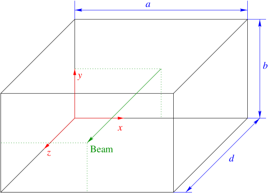
Figure 1: Sketch of the rectangular cavity; take note that coordinates of the beam axis are x=a/2 and y=b/2.

In order to simplify our calculations without loosing the general physical meaning, we shall consider a rectangular resonator, as the one shown in Fig.1, which is characterized [3] by the following field components:

$$B_{x}=-{B_{0}\over K_{c}^{2}}\left({m\pi\over a}\right)\left({p\pi\over d}\right)\sin\left({m\pi x\over a}\right)\cos\left({n\pi y\over b}\right)\cos\left({p\pi z\over d}\right)\cos\,\omega t$$ (32)

$$B_{y}=-{B_{0}\over K_{c}^{2}}\left({n\pi\over b}\right)\left({p\pi\over d}\right)\cos\left({m\pi x\over a}\right)\sin\left({n\pi y\over b}\right)\cos\left({p\pi z\over d}\right)\cos\,\omega t$$ (33)

$$B_{z}=B_{0}\cos\left({m\pi x\over a}\right)\cos\left({n\pi y\over b}\right)\sin\left({p\pi z\over d}\right)\cos\,\omega t$$ (34)

$$E_{x}=-B_{0}\left({n\pi\over b}\right){\omega\over K_{c}^{2}}\cos\left({m\pi x\over a}\right)\sin\left({n\pi y\over b}\right)\sin\left({p\pi z\over d}\right)\sin\,\omega t$$ (35)

$$E_{y}=B_{0}\left({n\pi\over b}\right){\omega\over K_{c}^{2}}\sin\left({m\pi x\over a}\right)\cos\left({n\pi y\over b}\right)\sin\left({p\pi z\over d}\right)\sin\,\omega t$$ (36)

$$E_{z}=0~{}~{}~{}({\mathrm{as~{}typical~{}for~{}a~{}TE~{}mode}})$$ (37)

where $B_{0}$ is the amplitude of the $B_{z}$-component and

$$K_{c}=\sqrt{\left({m\pi\over a}\right)^{2}+\left({n\pi\over b}\right)^{2}}$$ (38)

$${\omega\over c}=K={2\pi\over\lambda}=\sqrt{\left({m\pi\over a}\right)^{2}+\left({n\pi\over b}\right)^{2}+\left({p\pi\over d}\right)^{2}}$$ (39)

The wave’s phase velocity is $v_{\rm ph}=\beta_{\rm ph}c$ where

$$\beta_{\rm ph}={K\over\sqrt{K^{2}-K_{c}^{2}}}=\sqrt{1+\left({md\over pa}\right)^{2}+\left({nd\over pb}\right)^{2}}$$ (40)

We have to recall that the polarization of a beam, revolving in a ring whose guide field is $\vec{B}_{\mathrm{ring}}$, can be defined as

$$P={{N_{\uparrow}-N_{\downarrow}}\over{N_{\uparrow}+N_{\downarrow}}}$$ (41)

where $N_{\uparrow}$ = No. Particles Spin Up (e.g. parallel to $\vec{B}_{\mathrm{ring}}$)
$N_{\downarrow}$ = No. Particles Spin Down (antiparallel to $\vec{B}_{\mathrm{ring}}$)

and $P$ indicates the macroscopic average over the particle distribution in the beam, which is equivalent to the quantum mechanical expectation value found by means of the quantum statistical matrix. Obviously, an unpolarized beam has $P=0$ or $N_{\uparrow}$ = $N_{\downarrow}$.

A quick comparison among the SG-force components, given by the set of equations (26)-(31), suggests that $f_{z}$ will dominate at high energy, since it contains terms proportional to $\gamma^{2}$, whereas the transverse components have terms independent of $\gamma$, not to mention the $\gamma^{-1}$ terms.

The most appropriate choice of the spin orientation seems to be the one parallel to ${\hat{y}}$ i.e. to $\vec{B}_{\mathrm{ring}}$, i.e. the force component is the one given by eq. (28) with the insertion of eq. (30). This means that particles undergoing energy gain (or loss) don’t need any spin rotation while entering and leaving the rf cavity, beyond the advantage of having to deal with a force component proportional to $\gamma^{2}$. Choosing the simplest ${\mathrm{TE}}_{011}$ mode, the quantities (38), (39) and (40) reduce to

$$k_{c}={\pi\over b}$$ (42)

$$\omega=c\sqrt{\left({\pi\over b}\right)^{2}+\left({\pi\over d}\right)^{2}}$$ (43)

$$\beta_{\rm ph}=\sqrt{1+\left({d\over b}\right)^{2}}$$ (44)

Setting $x={a\over 2}$ and $y={b\over 2}$ the field components along the beam axis become

$$B_{x}=B_{z}=0$$ (45)

$$B_{y}=-B_{0}{b\over d}\,\cos\left({\pi z\over d}\right)\cos\,\omega t$$ (46)

$$E_{x}=-\omega\,B_{0}{b\over\pi}\,\sin\left({\pi z\over d}\right)\sin\,\omega t$$ (47)

$$E_{y}=E_{z}=0$$ (48)

therefore the force component $f_{z}$ can be written as

$$f_{z}=\mu^{*}\gamma^{2}B_{0}b\,\left\{{1\over\pi}\left[\left({\pi\over d}\right)^{2}+\left({\beta\omega\over c}\right)^{2}\right]\sin\left({\pi z\over d}\right)\cos\,\omega t+{2\over d}\left({\beta\omega\over c}\right)\cos\left({\pi z\over d}\right)\sin\,\omega t\right\}$$ (49)

For completeness, we shall also analyze the possibility of using a spin orientation parallel to ${\hat{z}}$, i.e. to the motion direction, even though this option requires a system of spin rotators and looses a factor of $\gamma$ in the force component.

5 Involved Energy

The energy gained, or lost, by a particle with a magnetic moment after having crossed a rf cavity can be evaluated by integrating the Stern-Gerlach force (22) over the cavity length, namely:

$$\Delta U=\int_{0}^{d}dU=\int_{0}^{d}\vec{f}\cdot d\vec{r}=\int_{0}^{d}f_{z}dz=\int_{0}^{d}\mu^{*}C_{zy}\,dz$$ (50)

Bearing in mind eq. (49) and carrying out the trivial substitution $\omega t={\omega z\over\beta c}$, the integral (50) becomes

$$\Delta U=\mu^{*}\gamma^{2}B_{0}b\,\left\{{1\over\pi}\left[\left({\pi\over d}\right)^{2}+\left({\beta\omega\over c}\right)^{2}\right]I_{1}+{2\over d}\left({\beta\omega\over c}\right)I_{2}\right\}$$

with

$$I_{1}=\int_{0}^{d}\sin\left({\pi z\over d}\right)\cos\left({\omega z\over\beta c}\right)dz={{\pi\over d}\over\left({\pi\over d}\right)^{2}-\left({\omega\over\beta c}\right)^{2}}\left[1+\cos\left({\omega d\over\beta c}\right)\right]$$

$$I_{2}=\int_{0}^{d}\cos\left({\pi z\over d}\right)\sin\left({\omega z\over\beta c}\right)dz=-{{\omega\over\beta c}\over\left({\pi\over d}\right)^{2}-\left({\omega\over\beta c}\right)^{2}}\left[1+\cos\left({\omega d\over\beta c}\right)\right]$$

or

$$\Delta U=\mu^{*}\gamma^{2}B_{0}\,{b\over d}\,{\left({\pi\over d}\right)^{2}+\left({\beta\omega\over c}\right)^{2}-2\left({\omega\over c}\right)^{2}\over\left({\pi\over d}\right)^{2}-\left({\omega\over\beta c}\right)^{2}}\left[1+\cos\left({\omega d\over\beta c}\right)\right]$$ (51)

Taking into account the stationary wave conditions (eqs. 43 and 44) pertaining to the $\rm TE_{011}$ mode, the length of the cavity can be expressed as

$$d={1\over 2}\beta_{\rm ph}\lambda$$ (52)

which allows us to write eq. (51) as

$$\Delta U=\gamma^{2}\beta^{2}\mu^{*}B_{0}\,{b\over d}\,{1+\beta_{\rm ph}^{2}(\beta^{2}-2)\over\beta^{2}-\beta_{\rm ph}^{2}}\left(1+\cos{\beta_{\rm ph}\over\beta}\pi\right)$$ (53)

In the ultrarelativistic limit ($\gamma\gg 1$ and $\beta\simeq 1$),

$$\Delta U\simeq\mu^{*}B_{0}\,{b\over d}\,\gamma^{2}(1+\cos\beta_{\rm ph}\pi)=2\,\mu^{*}B_{0}\,{b\over d}\,\gamma^{2}~{}~{}~{}(\beta_{\rm ph}={\hbox{even integer}})$$ (54)

As hinted before, let us evaluate the work-energy integral when the particle enters into the cavity with its spin parallel to $\hat{z}$. In this example we must choose the mode ${\mathrm{TE}}_{021}$ as the lowest one; then we have from eqs. (34) and (31) respectively

$$B_{z}=-B_{0}\,\sin\left({\pi z\over d}\right)\,\cos\,\omega t$$ (55)

$$f_{z}=\mu^{*}C_{zz}=-\mu^{*}\gamma B_{0}\left[{\pi\over d}\cos\left({\pi z\over d}\right)\cos\,\omega t-\left({\beta\omega\over c}\right)\sin\left({\pi z\over d}\right)\cos\,\omega t\right]$$ (56)

and proceeding as above we obtain

$$\Delta U=\mu^{*}B_{0}\gamma\,{\pi\over d}\,{{\omega\over\beta c}-{\beta c\over\omega}\over\left({\pi\over d}\right)^{2}-\left({\omega\over\beta c}\right)^{2}}\sin\left({\omega d\over\beta c}\right)$$ (57)

and

$$\Delta U={\mu^{*}B_{0}\over\gamma}{\beta_{\rm ph}\beta\over\beta_{\rm ph}^{2}-\beta^{2}}\sin\left({\beta_{\rm ph}\over\beta}\pi\right)$$ (58)

or ultrarelativistically

$$\Delta U\simeq{\mu^{*}B_{0}\over\gamma}{\beta_{\rm ph}\over\beta_{\rm ph}^{2}-1}\sin\beta_{\rm ph}\pi,\qquad\Delta U_{\rm max}\sim-1.62{\mu^{*}B_{0}\over\gamma}\quad(\hbox{when $\beta_{\rm ph}\sim 1.13$})$$ (59)

confirming a result [4] already achieved.

Before making up our mind, we need to compare the energy gain/loss due to the Stern-Gerlach interaction with the same quantity caused by the electric field. To this aim, we emphasize that

$$dU_{E}=\vec{f}_{E}\cdot d\vec{r}=eE_{x}dx$$ (60)

as can be easily understood looking at eqs. (47) and (48). Since the carrier particle travels from 0 to $d$ along the $z$-axis, the only integral which makes sense is the following:

$$\Delta U_{E}=\int_{0}^{d}eE_{x}\,dx=\int_{0}^{d}eE_{x}\,{dx\over dz}dz=\int_{0}^{d}eE_{x}\,x^{\prime}dz$$ (61)

or

$$\Delta U_{E}=-x^{\prime}e\omega B_{0}{b\over\pi}\int_{0}^{d}\sin\left({\pi z\over d}\right)\sin\left({\omega z\over\beta c}\right)dz=-x^{\prime}e\omega B_{0}{b\over d}{\sin\left({\omega d\over\beta c}\right)\over\left({\pi\over d}\right)^{2}-\left({\omega\over\beta c}\right)^{2}}$$

or

$$\Delta U_{E}=\left[e\omega B_{0}{bd\over\pi^{2}}{\beta^{2}\over\beta_{\rm ph}^{2}-\beta^{2}}\sin{\beta_{\rm ph}\over\beta}\pi\right]x^{\prime}=\kappa x^{\prime}$$ (62)

having proceeded as before.

We recall that the Stern-Gerlach interaction in the realm of particle accelerators has been proposed either for separating in energy particles with opposite spin states, the well known [5] spin-splitter concept, or for settling an absolute polarimeter [6].

As far as the spin-splitter is concerned, we quickly recall that spin up particles receive (or loose) that amount of energy given by eq. (54) at each rf cavity crossing, and this will take place all over the time required. Simultaneously, spin down particles behave exactly in the opposite way, i.e. they loose (or gain) the same amount of energy turn after turn. The actual most important issue is that the energy exchanges sum up coherently. More quantitatively, we may indicate as the final energy separation after $N$ revolutions:

$$\Delta_{\uparrow\downarrow}=\sum\,\{\Delta_{\uparrow}-(-\Delta_{\downarrow})\}=4{b\over d}N\,\mu^{*}B_{0}\,\gamma^{2}\simeq 4\,N\,\mu^{*}B_{0}\,\gamma^{2}$$ (63)

Instead, the adding up of the energy contribution (62) due to the electric field is

$$(\Delta U_{E})_{tot}=\sum\,\Delta U_{E}=\kappa\,\sum\,x^{\prime}=0$$ (64)

since $x^{\prime}$ changes continuously its sign with a periodicity related to the period of the betatron oscillations.

The result (63), together with the demonstration (64), would seem to provide very good news for the spin-splitter method!

As far as the polarimeter is concerned, we have to bear in mind that we are interested in the instantaneous interaction between magnetic moment and the rf fields: therefore the zero-averaging due to the incoherence of the betatron oscillations would not help us. Notwithstanding, if we set $\beta_{\rm ph}$ equal to an integer in eq. (62), we have for U.R. particles:

$$\Delta U_{E}={x^{\prime}e\omega B_{0}\,bd\over\pi^{2}(\beta_{\rm ph}^{2}-1)}\sin\left(\beta_{\rm ph}\pi+{\beta_{\rm ph}\pi\over 2\gamma^{2}}\right)\simeq\pm{x^{\prime}bd\over 2\pi}{\beta_{\rm ph}\over\beta_{\rm ph}^{2}-1}{e\omega B_{0}\over\gamma^{2}}$$ (65)

Then this $1/\gamma^{2}$ dependence of the spurious signal, compared to the $\gamma^{2}$ dependence of the signal (54) to be measured, sounds interesting for the feasibility of this kind of polarimeter; however, one must realize that if $\beta_{\rm ph}$ is not exactly an integer, then eq. (65) would become

$$\Delta U_{E}\sim\pm{x^{\prime}bd\over 2\pi}{e\omega B_{0}\over\beta_{\rm ph}^{2}-1}\left(\epsilon+{\beta_{\rm ph}\over\gamma^{2}}\right)$$ (66)

where $\epsilon$ is the error in $\beta_{\rm ph}$.

6 A Few Numerical Examples

The spin-splitter principle requires a repetitive crossing of $N_{\rm cav}$ cavities distributed along the ring, each of them resonating in the TE mode. After each revolution, the particle experiences a variation, or kick, of its energy or of its momentum spread

$$\zeta={\delta p\over p}={1\over\beta^{2}}{\delta E\over E}\simeq{N_{\rm cav}\Delta U\over E}\simeq{2\sqrt{3}\over 3}\,N_{\rm cav}{B_{0}\over B_{\infty}}\gamma$$ (67)

having made use of eq. (54), further simplified by reasonably setting $\beta_{\rm ph}=2$, and with

$$B_{\infty}={mc^{2}\over\mu^{*}}={1.503\times 10^{-10}~{}{\rm J}\over 1.41\times 10^{-26}~{}{\rm JT}^{-1}}\simeq 10^{16}~{}{\rm T}$$ (68)

for (anti)protons. From eq. (67) we may find as the number of turns needed for attaining a momentum separation equal to 2$\left({\Delta p\over p}\right)$

$$N_{\rm SS}={\left({\Delta p\over p}\right)\over\zeta}={\sqrt{3}\over 2\,N_{\rm cav}\gamma}{B_{\infty}\over B_{0}}\left({\Delta p\over p}\right)$$ (69)

Multiplying $N_{\rm SS}$ by the revolution period $\tau_{\rm rev}$ we obtain

$$\Delta t=N_{\rm SS}\tau_{\rm rev}$$ (70)

as the actual time spent in this operation. For the sake of having some data, we consider RHIC [7] and HERA [8] whose essential parameters are shown in Table I together with what can be found by making use of eqs. (69) and (70) where $B_{0}\simeq 0.1~{}T$ and $N_{\rm cav}=200$ are chosen as realistic values.

Table I: RHIC and HERA parameters

	RHIC	HERA
E(GeV)	250	820
$\gamma$	266.5	874.2
$\tau_{\rm rev}(\mu\rm s)$	12.8	21.1
${\Delta p\over p}$	$4.1\times 10^{-3}$	$5\times 10^{-5}$
$N_{\rm SS}$	$6.67\times 10^{9}$	$2.48\times 10^{7}$
$\Delta t$	$8.52\times 10^{4}~{}s\,\simeq\,23.7~{}h$	523   s

In the example of the polarimeter we have to pick up a signal generated at each cavity crossing. Therefore, making use of eq. (54) we have for a bunch train made up of $N$ particles the total energy transfer

$$\Delta U\approx 2NP\mu^{*}B_{0}\,\frac{b}{d}\,\gamma^{2}$$ (71)

where $P$ is the beam polarization slightly modified with respect the definition (41)

$$P={{N_{\rightarrow}-N_{\leftarrow}}\over{N_{\rightarrow}+N_{\leftarrow}}}$$ (72)

The average power transferred will be

$$W=\frac{\Delta U}{\tau_{\rm rev}}$$ (73)

If we operate our cavity as a parametric converter [9][10], with an initially empty level, we have for the power transferred to this empty level

$$W_{2}=\frac{\omega_{\rm rf}}{\omega_{\rm rev}}\,W=\frac{\nu_{\rm rf}}{\nu_{\rm rev}}\,W$$ (74)

where $\nu_{\rm rf}$ is the working frequency of the resonant cavity (typically in the GHz range), and $\nu_{\rm rev}$ is the revolution frequency. Putting all together we have

$$W_{2}\simeq 2\,P\,\frac{\nu_{\rm rf}}{\nu_{\rm rev}}\,\mu^{*}B_{0}\,\frac{b}{d}\,\gamma^{2}$$ (75)

A feasibility test of the polarimeter principle has been proposed [6] and studied [11] to be carried out in the 500 MeV electron ring [12] of MIT- Bates, whose main characteristics are

Table II: MIT-Bates parameters

$\tau_{\rm rev}$	634 nsec
$\nu_{\rm rev}$	1.576 MHz
$N_{electrons}$	$3.6\times 10^{8}\cdot 225=8.1\times 10^{10}$
$\gamma$	$\simeq 10^{3}$
$b/d$	$\sqrt{3}/3$
$B_{0}$	$\simeq 0.1$ T
$\nu_{\rm rf}/\nu_{\rm rev}$	$\approx 10^{3}$
$\mu^{*}$	$9.27\times 10^{-24}~{}{\rm JT}^{-1}$

and, since polarized electrons can be injected into this ring but precessing on a horizontal plane, the ${\mathrm{TE}}_{101}$ mode is more appropriate than the ${\mathrm{TE}}_{011}$ as we shall have to use $B_{x}$ rather than $B_{y}$: a choice that does not make any substantial difference! From the above data we obtain

$$W_{2}\simeq 137P\,{\rm watts}$$ (76)

Paradoxically, even for an almost unpolarized beam with $N_{\rightarrow}-N_{\leftarrow}=1$ and, as a consequence of eq. (72), with $P\simeq 1.23\times 10^{-11}$, we should obtain $W_{2}\approx 1.7~{}{\rm nW}$, which can be easily measured.

As a last check, let us compare the energy exchanges ($\vec{\mu}\Leftrightarrow\vec{B}$) and ($e\Leftrightarrow\vec{E}$). Taking into account eqs. (52), (54) and (65), and setting $x^{\prime}\simeq 1~{}\rm mrad$, $\beta_{\rm ph}=2$ and $\lambda=10~{}\rm cm$, we have for the Bates-MIT ring:

$$r=\frac{\Delta U_{E}}{\Delta U}=\frac{x^{\prime}}{8}\,\frac{\beta_{\rm ph}^{3}}{\beta_{\rm ph}^{2}-1}\,\frac{\lambda ec}{\mu^{*}}\,\frac{1}{\gamma^{4}}=1.72\times 10^{-4}$$ (77)

i.e. the spurious signal, depending upon the electric interaction between $e$ and $\vec{E}$, is absolutely negligible with respect the measurable signal generated by the magnetic interaction.

7 Conclusions

There is not too much to add to what has been found in the previous Sections, aside from performing more accurate calculations and numerical simulations. The Stern-Gerlach interaction seems very promising either for attaining the self polarization of a $p(\bar{p})$ beam or for realizing an absolute polarimeter.

In the first example the problem raised [13] by the rf filamentation still holds on, although some tricks can be conceived: the extreme one could be the implementation of a triangular waveform in the TM cavity which bunches the beam.

The second example requires nothing but to implement that experimental test at the Bates-MIT electron ring.

References

• [1] Synge, Relativity: The Special Theory, North Holland Publ. Co., Amsterdam, 1956.
• [2] J. D. Jackson, Classical Electrodynamics, John Wiley and & Sons, New York, 1975.
• [3] S. Ramo, J. R. Whinnery and T. Van Duzer, Fields and Waves in Communication Electronics, John Wiley and & Sons, New York, 1965.
• [4] W. W. MacKay, “Notes on a Generalization of the Stern-Gerlach Force”, RHIC/AP/153, April 6 1998, and W. W. MacKay, “Converging towards a Solution of $\gamma$ vs $1/\gamma$” RHIC/AP/175, June 1999.
• [5] M. Conte, A. Penzo and M. Pusterla, Il Nuovo Cimento, A108 (1995) 127.
• [6] P. Cameron et al., “An RF Resonant Polarimeter Phase 1 Proof-of-Principle Experiment”, RHIC/AP/126, January 6 1998.
• [7] M. A. Harrison, “The RHIC Project”, Proceedings of EPAC96, p. 13, Sitges (Barcelona), 1996.
• [8] E. Gianfelice-Wendt, “HERA Upgrade Plans”, Proc. of EPAC98, p. 118, Stolkholm (1998).
• [9] J. M. Manley, H. E. Rowe, “Some General Properties of Nonlinear Elements - Part I. General Energy Relations”, Proceedings of the IRE, 44 (1956) 904.
• [10] W. H. Louisell, Coupled Modes and Parametric Electronics, John Wiley & Sons, New York, 1965.
• [11] M. Ferro, Thesis of Degree, Genoa University, April 22 1999.
• [12] K. D. Jacobs et al., “Commissioning the MIT-Bates South Hall Ring”, Proceedings PAC1, 1995.
• [13] M. Conte, W. W. MacKay and R. Parodi, “An Overview of the Longitudinal Stern-Gerlach Effect”, BNL-52541, UC-414, November 17 1997.