1 Problem

In the usual formulation of the Kirchhoff diffraction integral, a scalar field with harmonic time dependence at frequency $\omega$ is deduced at the interior of a charge-free volume from knowledge of the field (or its normal derivative) on the bounding surface. In particular, the field is propagated forwards in time from the boundary to the desired observation point.

Construct a time-reversed version of the Kirchhoff integral in which the knowledge of the field on the boundary is propagated backwards in time into the interior of the volume.

Consider the example of an optical focus at the origin for a system with the $z$ axis as the optic axis. In the far field beyond the focus a Gaussian beam has cone angle $\theta_{0}\equiv\sqrt{2}\sigma_{\theta}$, and the $x$ component of the electric field in a spherical coordinate system is given approximately by

$$E_{x}(r,\theta,\phi,t)=E(r)e^{i(kr-\omega t)}e^{-\theta^{2}/\theta_{0}^{2}},$$ (1)

where $k=\omega/c$ and $c$ is the speed of light. Deduce the field near the focus.

Since the Kirchhoff diffraction formalism requires the volume to be charge free, the time-reversed technique is not applicable to cases where the source of the field is inside the volume. Nonetheless, the reader may find it instructive to attempt to apply the time-reversed diffraction integral to the example of an oscillating dipole at the origin.

2 The Kirchhoff Integral via Green’s Theorem

A standard formulation of Kirchhoff’s diffraction integral for a scalar field $\psi({\bf x})$ with time dependence $e^{-i\omega t}$ is

$$\psi({\bf x})\approx{k\over 2\pi i}\int_{S}{e^{ikr^{\prime}}\over r^{\prime}}\psi({\bf x}^{\prime})d{\rm Area}^{\prime},$$ (2)

where the spherical waves $e^{i(kr^{\prime}-\omega t)}/r^{\prime}$ are outgoing, and $r^{\prime}$ is the magnitude of vector ${\bf r}^{\prime}={\bf x}-{\bf x}^{\prime}$.

For a time-reversed formulation in which we retain the time dependence as $e^{-i\omega t}$, the spherical waves of interest are the incoming waves $e^{-i(kr^{\prime}+\omega t)}/r^{\prime}$. In brief, the desired time-reversed diffraction integral is obtained from eq. (2) on replacing $i$ by $-i$:

$$\psi({\bf x})\approx{ik\over 2\pi}\int_{S}{e^{-ikr^{\prime}}\over r^{\prime}}\psi({\bf x}^{\prime})d{\rm Area}^{\prime}.$$ (3)

For completeness, we review the derivation of eqs. (2)-(3) via Green’s theorem. See also, sec. 10.5 of ref. [1].

Green tells us that for any two well-behaved scalar fields $\phi$ and $\psi$,

$$\int_{V}(\phi\nabla^{2}\psi-\psi\nabla^{2}\phi)d{\rm Vol}=\int_{S}(\phi\nabla^{\prime}\psi-\psi\nabla^{\prime}\phi)\cdot d{\bf S}^{\prime}.$$ (4)

The surface element $d{\bf S}^{\prime}$ is directly outward from surface $S$. We consider fields with harmonic time dependence at frequency $\omega$, and assume the factor $e^{-i\omega t}$. The wave function of interest, $\psi$, is assumed to have no sources within volume $V$, and so obeys the Helmholtz wave equation,

$$\nabla^{2}\psi+k^{2}\psi=0.$$ (5)

We choose function $\phi({\bf x})$ to correspond to waves associated with a point source at ${\bf x}^{\prime}$. That is,

$$\nabla^{2}\phi+k^{2}\phi=-\delta^{3}({\bf x}-{\bf x}^{\prime}).$$ (6)

The well-known solutions to this are the incoming and outgoing spherical waves,

$$\phi_{\pm}({\bf x},{\bf x}^{\prime})={e^{\pm ikr^{\prime}}\over r^{\prime}},$$ (7)

where the + sign corresponds to the outgoing wave. We recall that

$$\nabla^{\prime}r^{\prime}=-{{\bf r}^{\prime}\over r^{\prime}}=-\hat{\bf n}_{o},$$ (8)

where $\hat{\bf n}_{o}$ points towards the observer at x. Then,

$$\nabla^{\prime}\phi_{\pm}=\mp ik\hat{\bf n}_{o}\left(1\pm{1\over ikr^{\prime}}\right)\phi.$$ (9)

Inserting eqs. (5)-(9) into eq. (4), we find

$$\psi({\bf x})=-{1\over 4\pi}\int_{S}{e^{\pm ikr^{\prime}}\over r^{\prime}}\hat{\bf n}^{\prime}\cdot\left[\nabla^{\prime}\psi\pm ik\hat{\bf n}_{o}\left(1\pm{1\over ikr^{\prime}}\right)\psi\right]d{\rm Area}^{\prime},$$ (10)

where the overall minus sign holds with the convention that $\hat{\bf n}^{\prime}$ is the inward normal to the surface.

We only consider cases where the source of the wave $\psi$ is far from the boundary surface, so that on the boundary $\psi$ is well approximated as a spherical wave,

$$\psi({\bf x}^{\prime})\approx A{e^{ikr_{s}}\over r_{s}},$$ (11)

where $r_{s}$ is the magnitude of the vector ${\bf r}_{s}={\bf x}^{\prime}-{\bf x}_{s}$ from the effective source point ${\bf x}_{s}$ to the point ${\bf x}^{\prime}$ on the boundary surface. In this case,

$$\nabla^{\prime}\psi=ik\hat{\bf n}_{s}\left(1\pm{1\over ikr_{s}}\right)\psi,$$ (12)

where $\hat{\bf n}_{s}={\bf r_{s}}/r_{s}$

We also suppose that the observation point is far from the boundary surface, so that $kr^{\prime}\ll 1$ as well as $kr_{s}\ll 1$. Hence, we neglect the terms in $1/ikr^{\prime}$ and $1/ikr_{s}$ to find

$$\psi({\bf x})=-{ik\over 4\pi}\int_{S}{e^{\pm ikr^{\prime}}\over r^{\prime}}\hat{\bf n}^{\prime}\cdot(\hat{\bf n}_{s}\pm\hat{\bf n}_{o})\psi({\bf x}^{\prime})d{\rm Area}^{\prime}.$$ (13)

The usual formulation, eq. (2), of Kirchhoff’s law is obtained using outgoing waves (+ sign), and the paraxial approximation that $\hat{\bf n}^{\prime}\approx\hat{\bf n}_{o}\approx\hat{\bf n}_{s}$. The latter tacitly assumes that the effective source is outside volume $V$.

Here, we are interested in the case where the effective source is inside the volume $V$, so that the paraxial approximation is $\hat{\bf n}^{\prime}\approx\hat{\bf n}_{o}\approx-\hat{\bf n}_{s}$. When we use the incoming wave function to reconstruct $\psi({\bf x},t)$ from information on the boundary at time $t^{\prime}>t$, we use the $-$ sign in eq. (13) to find eq. (3).

Note that in this derivation, we assumed that $\psi$ obeyed eq. (5) throughout volume $V$, and so the actual source of $\psi$ cannot be within $V$. Our time-reversed Kirchhoff integral (3) can only be applied when any source inside $V$ is virtual. This includes the interesting case of a focus of an optical system (secs. 4 and 5). However, we cannot expect eq. (3) to apply to the case of a physical source, such as an oscillating dipole, inside volume $V$ (sec. 6). The laws of diffraction do not permit electromagnetic waves to converge into a volume smaller than a wavelength cubed, and so eq. (3) cannot be expected to describe the near fields around a source smaller than this.

3 A Plane Wave

The time-reversed Kirchhoff integral (3) for the $x$ component of the electric field is

$$E_{x}({\rm obs,now})={ik\over 2\pi}\int{e^{-ikr^{\prime}}\over r^{\prime}}E_{x}(r,\theta,\phi,\rm future)d{\rm Area},$$ (14)

where $r^{\prime}$ is the distance from the observation point ${\bf r}_{\rm obs}=(x,y,z)$ in rectangular coordinates to a point ${\bf r}=r(\sin\theta\cos\phi,\sin\theta\sin\phi,\cos\theta)$ on a sphere of radius $r$ in the far field.

As a first example, consider a plane electromagnetic wave,

$$E_{x}=E_{0}e^{i(kz-\omega t)}=E_{0}e^{i(kr\cos\theta-\omega t)},$$ (15)

where the second form holds in a spherical coordinate system $(r,\theta,\phi)$ where $\theta$ is measured with respect to the $z$ axis. We take the point of observation to be $(x,y,z)=(0,0,r_{0})$, and evaluate the diffraction integral (14) over a sphere of radius $r\gg r_{0}$. In the exponential factor in the Kirchhoff integral, we approximate $r^{\prime}$ as

$$r^{\prime}\approx r-\hat{\bf r}\cdot{\bf r}_{\rm obs}=r-r_{0}\cos\theta,$$ (16)

while in the denominator we approximate $r^{\prime}$ as $r$. Then,

$$E_{x}({\rm obs}) \approx {ik\over 2\pi}\int_{-1}^{1}r^{2}d\cos\theta\int_{0}^{2\pi}d\phi\ {e^{-ik(r-r_{0}\cos\theta)}\over r}E_{0}e^{ikr\cos\theta}$$

$$= {r\over r+r_{0}}E_{0}[e^{ikr_{0}}-e^{-ik(2r+r_{0})}]$$

$$\approx E_{0}e^{ikr_{0}},$$

where we ignore the rapidly oscillating term $e^{-ik(2r+r_{0})}$ as unphysical.

This verifies that the time-reversed diffraction formula works for a simple example.

4 The Transverse Field near a Laser Focus

We now consider the far field of a laser beam whose optic axis is the $z$ axis with focal point at the origin. The polarization is along the $x$ axis, and the electric field has Gaussian dependence on polar angle with characteristic angle $\theta_{0}\ll 1$. Then, we can write

$$E_{x}(r,\theta,\phi)=E(r)e^{ikr}e^{-\theta^{2}/\theta_{0}^{2}},$$ (18)

where $E(r)$ is the magnitude of the electric field on the optic axis at distance $r$ from the focus. In the exponential factor in the Kirchhoff integral (14), $r^{\prime}$ is the distance from the observation point ${\bf r}_{|rmobs}=(x,y,z)$ to a point ${\bf r}=r(\sin\theta\cos\phi,\sin\theta\sin\phi,\cos\theta)$ on the sphere. We approximate $r^{\prime}$ as

$$r^{\prime}\approx r-\hat{\bf r}\cdot{\bf r}_{\rm obs}=r-x\sin\theta\cos\phi-y\sin\theta\sin\phi-z\cos\theta,$$ (19)

while in the denominator we approximate $r^{\prime}$ as $r$. Inserting eqs. (18) and (19) into (14), we find

$$E_{x}({\rm obs}) = {ikrE(r)\over 2\pi}\int_{-1}^{1}e^{ikz\cos\theta}e^{-\theta^{2}/\theta_{0}^{2}}d\cos\theta\int_{0}^{2\pi}e^{ikx\sin\theta\cos\phi+iky\sin\theta\sin\phi}d\phi$$ (20)

$$= ikrE(r)\int_{-1}^{1}e^{ikz\cos\theta}e^{-\theta^{2}/\theta_{0}^{2}}J_{0}(k\rho\sin\theta)d\cos\theta,$$

where

$$\rho=\sqrt{x^{2}+y^{2}},$$ (21)

and $J_{0}$ is the Bessel function of order zero.

Since we assume that the characteristic angle $\theta_{0}$ of the laser beam is small, we can approximate $\cos\theta$ as $1-\theta^{2}/2$ and $k\rho\sin\theta$ as $k\rho\theta$. Then, we have

$$E_{x}({\rm obs}) \approx ikrE(r)e^{ikz}\int_{0}^{\infty}e^{-(2/\theta_{0}^{2}+ikz)\theta^{2}/2}J_{0}\left(\sqrt{2}k\rho\sqrt{\theta^{2}/2}\right)d(\theta^{2}/2)$$ (22)

$$= {ik\theta_{0}^{2}rE(r)e^{ikz}e^{-k^{2}\theta_{0}^{2}\rho^{2}/4(1+ik\theta_{0}^{2}z/2)}\over 2(1+ik\theta_{0}^{2}z/2)},$$

where the Laplace transform, which is given explicitly in [2], can be evaluated using the series expansion for the Bessel function. This expression can be put in a more familiar form by introducing the Rayleigh range (depth of focus),

$$z_{0}={2\over k\theta_{0}^{2}},$$ (23)

and the so-called waist of the laser beam,

$$w_{0}=\theta_{0}z_{0}={2\over k\theta_{0}}.$$ (24)

We define the electric field strength at the focus $(\rho=0,z=0)$ to be $E_{0}$, so we learn that the far-field strength is related by

$$E(r)=-i{z_{0}\over r}E_{0}.$$ (25)

The factor $-i=e^{-i\pi/2}$ is the $90^{\circ}$ Guoy phase shift between the focus and the far field. Then, the transverse component of the electric field near the focus is

$$E_{x}(x,y,z) \approx E_{0}{e^{-\rho^{2}/w_{0}^{2}(1+iz/z_{0})}e^{ikz}\over(1+iz/z_{0})}$$ (26)

$$= E_{0}{e^{-\rho^{2}/w_{0}^{2}(1+z^{2}/z_{0}^{2})}e^{-i\tan^{-1}z/z_{0}}e^{i\rho^{2}z/w_{0}^{2}z_{0}(1+z^{2}/z_{0}^{2})}e^{ikz}\over\sqrt{1+(z/z_{0})^{2}}}.$$

This is the usual form for the lowest-order mode of a linearly polarized Gaussian laser beam [3]. Figure 1 plots this field.

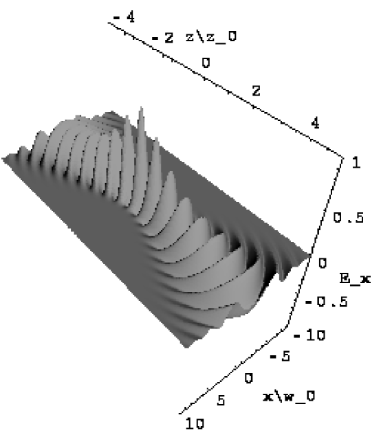
Figure 1: The electric field $E_{x}(x,0,z)$ of a linearly polarized Gaussian beam with diffraction angle $\theta_{0}=0.45$.

The Gaussian beam (26) could also be deduced by a similar argument using eq. (2), starting from the far field of the laser before the focus. The form (26) is symmetric in $z$ except for a phase factor, and so is a solution to the problem of transporting a wave from $z=-r$ to $z=+r$ such that the functional dependence on $\rho$ and $z$ is invariant up to a phase factor. One of the earliest derivations [4] of the Gaussian beam was based on the formulation of this problem as an integral equation for the eigenfunction (26).

5 The Longitudinal Field

Far from the focus, the electric field E(r) is perpendicular to the radius vector r. For a field linearly polarized in the $x$ direction, there must also be a longitudinal component $E_{z}$ related by

$${\bf E}\cdot\hat{\bf r}=E_{x}\sin\theta\cos\phi+E_{z}\cos\theta=0.$$ (27)

Thus, far from the focus,

$$E_{z}({\bf r})=-E_{x}({\bf r})\tan\theta\cos\phi.$$ (28)

Then, similarly to eqs. (14) and (20), we have

$$E_{z}({\rm obs}) = {ik\over 2\pi}\int{e^{-ikr^{\prime}}\over r^{\prime}}E_{z}({\bf r})d{\rm Area}$$ (29)

$$= -{ikrE(r)\over 2\pi}\int_{-1}^{1}e^{ikz\cos\theta}e^{-\theta^{2}/\theta_{0}^{2}}\tan\theta d\cos\theta\int_{0}^{2\pi}e^{ikx\sin\theta\cos\phi+iky\sin\theta\sin\phi}\cos\phi d\phi$$

$$= -{ikxz_{0}E_{0}\over\rho}\int_{-1}^{1}e^{ikz\cos\theta}e^{-\theta^{2}/\theta_{0}^{2}}\tan\theta J_{1}(k\rho\sin\theta)d\cos\theta,$$

using eq. (3.937.2) of [5].

We again note that the integrand is significant only for small $\theta$, so we can approximate eq. (29) as the Laplace transform

$$E_{z}(x,y,z) \approx -ik^{2}xz_{0}E_{0}e^{ikz}\sqrt{2}\int_{0}^{\infty}e^{-(2/\theta_{0}^{2}+ikz)\theta^{2}/2}\sqrt{\theta^{2}/2}J_{1}\left(\sqrt{2}k\rho\sqrt{\theta^{2}/2}\right)d(\theta^{2}/2)$$ (30)

$$= -{ik^{2}\theta_{0}^{4}xz_{0}E_{0}e^{ikz}e^{-\rho^{2}/w_{0}^{2}(1+iz/z_{0})}\over 4(1+iz/z_{0})^{2}}$$

$$= -i\theta_{0}{x\over w_{0}}{E_{x}(x,y,z)\over(1+iz/z_{0})},$$

with $E_{x}$ given by eq. (26). Figure 2 plots this field.

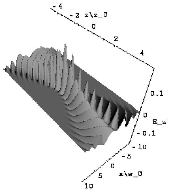
Figure 2: The electric field $E_{z}(x,0,z)$ of a linearly polarized Gaussian beam with diffraction angle $\theta_{0}=0.45$.

Together, the electric field components given by eqs. (26) and (30) satisfy the Maxwell equation $\nabla\cdot{\bf E}=0$ to order $\theta_{0}^{2}$ [6, 7, 8].

6 Oscillating Dipole at the Origin

We cannot expect the Kirchhoff diffraction integral to apply to the example of an oscillating dipole, if our bounding surface surrounds the dipole. Let us see what happens if we try to use eq. (3) anyway.

The dipole is taken to be at the origin, with moment $p$ along the $x$ axis. Then, the $x$ component of the radiation field is

$$E_{x}=k^{2}p\sin\theta_{x}{e^{ikr}\over r}.$$ (31)

where $\theta_{x}$ is the angle between the $x$ axis and a radius vector to the observer. We consider an observer near the origin at $(x,y,z)=(0,0,r_{0})$, for which $\sin\theta_{x}=1$, and so

$$E_{x}({\rm obs})=k^{2}p{e^{ikr_{0}}\over r_{0}}.$$ (32)

We now attempt to reconstruct this field near the origin from its value on a sphere of radius $r$ using the time-reversed Kirchhoff integral (3). We use a spherical coordinate system $(r,\theta,\phi)$ that favors the $z$ axis. Then, the $x$ component of the radiation field on the sphere of radius $r$ is

$$E_{x}(r,\theta,\phi)=k^{2}p\sqrt{1-\sin^{2}\theta\cos^{2}\phi}{e^{ikr}\over r}.$$ (33)

This form cannot be integrated analytically, so we use a Taylor expansion of the square root, which will lead to an expansion in powers of $1/r_{0}$. It turns out that the coefficient of the $1/r_{0}$ term, which is our main interest, is very close to that if we simply approximate the square root by unity. For brevity, we write

$$E_{x}(r,\theta,\phi)\approx k^{2}p{e^{ikr}\over r}.$$ (34)

In the time-reversed Kirchhoff integral (3), we make the usual approximation that $r^{\prime}=r-r_{0}\cos\theta$ in the exponential factor, but $r^{\prime}=r$ in the denominator. Then, using eq. (34) we have

$$E_{x}({\rm obs}) \approx {ik^{3}pe^{-ikr}\over 2\pi r}\int_{-1}^{1}r^{2}d\cos\theta\int_{0}^{2\pi}d\phi e^{ikr_{0}\cos\theta}{e^{ikr}\over r}$$ (35)

$$= k^{2}p{e^{ikr_{0}}\over r_{0}}-k^{2}p{e^{-ikr_{0}}\over r_{0}}$$

$$= 2ik^{3}p{\sin kr_{0}\over kr_{0}}.$$

The first, outgoing wave in middle line of eq. (35) is the desired form, but the second, incoming wave is of the same magnitude. Together, they lead to the form $\sin(kr_{0})/kr_{0}$ which is nearly constant for $kr_{0}\mathrel{\vbox{\kern 0.0pt\hbox{$<$} \kern 0.0pt\hbox{$\sim$} }}1$. The presence of outgoing as well as incoming waves is to be expected because dipole radiation is azimuthally symmetric about the $x$ axis. In the absence of a charged source at the origin, an outgoing wave at $\theta=\pi$ must correspond to an incoming wave at $\theta=0$.

The result that the reconstructed field is uniform for distances within a wavelength of the origin is consistent with the laws of diffraction that electromagnetic waves cannot be focused to a region smaller than a wavelength. Far fields of the form (31) could only be propagated back to the form of dipole fields near the origin with the addition of nonradiation fields tied to a charge at the origin. Such a construction is outside the scope of optics and diffraction.

References

[1]
J.D. Jackson,
Classical Electrodynamics, 3d ed. (Wiley, New York, 1999).
[2]
W. Magnus and F. Oberhettinger,
Functions of Mathematical Physics
(Springer-Verlag, Berlin, 1943; reprinted by Chelsea Publishing Company,
New York, 1949), pp. 131-132.
[3]
See, for example, sec. 14.5 of P.W. Milonni and J.H. Eberly,
Lasers
(Wiley Interscience, New York, 1988).
[4]
G.D. Boyd and J.P. Gordon,
Confocal Multimode Resonator for Millimeter Through Optical Wavelength
Masers,
Bell Sys. Tech. J. 40, 489-509 (1961).
[5]
I.S. Gradshteyn and I.M. Ryzhik,
Table of Integrals, Series, and Products, 5th ed. (Academic Press, San Diego, 1994).
[6]
M. Lax, W.H. Louisell and W.B. McKnight,
From Maxwell to paraxial wave optics,
Phys. Rev. A 11, 1365-1370 (1975).
[7]
L.W. Davis,
Theory of electromagnetic beams,
Phys. Rev. A 19, 1177-1179 (1979).
[8]
J.P. Barton and D.R. Alexander,
Fifth-order corrected electromagnetic field components for a fundamental
Gaussian beam,
J. Appl. Phys. 66, 2800-2802 (1989).