The Force-Velocity Relation for Growing Biopolymers

Abstract

The process of force generation by the growth of biopolymers is simulated via a Langevin-dynamics approach. The interaction forces are taken to have simple forms that favor the growth of straight fibers from solution. The force-velocity relation is obtained from the simulations for two versions of the monomer-monomer force field. It is found that the growth rate drops off more rapidly with applied force than expected from the simplest theories based on thermal motion of the obstacle. The discrepancies amount to a factor of three or more when the applied force exceeds $2.5~{}kT/a$, where $a$ is the step size for the polymer growth. These results are explained on the basis of restricted diffusion of monomers near the fiber tip. It is also found that the mobility of the obstacle has little effect on the growth rate, over a broad range.

]

I Introduction

The growth of biopolymers is a key ingredient in the crawling motion and internal transport processes of almost all eukaryotic cells. They crawl among each other and over substrates by motion of the cytoplasm into protrusions known as lamellipodia, filopodia, or microspikes according to their shapes. The forces driving the extension of these protusions are believed to comes from the growth of a collection of fibers assembled from monomers of the protein actin. The actin fibers are approximately 7 nm in diameter. With no opposing force, they can grow at velocities[1] of over $1~{}\mu$m/sec at physiological actin concentrations[2, 3] of 10–50$\mu$M; the velocities of the cell protrusions are typically[4, 5] in the range of $0.1~{}\mu$m/sec. Actin fiber growth also can power the motion of bacteria and viruses through the cell cytoplasm. The velocities usually range from $0.02$ to $0.2~{}\mu$m/sec, but velocities up to $1.5~{}\mu$m/sec have been observed. As they move, they leave behind “comet tails” made up of actin fibers[6, 7]. Recent experiments have studied the minimal ingredients necessary for such propulsion. For example, Ref. [8] shows that polystyrene beads coated with a catalytic agent for actin polymerization spontaneously move in cell extracts at velocities of $0.01$ to $0.05~{}\mu$m/sec, forming comet tails similar to those caused by bacteria and viruses. It has also been shown recently that Listeria and Shigella bacteria can move in a medium much simpler than a cell extract, containing in addition to actin monomers only the proteins Arp2/3 complex, actin depolymerizing factor, and capping protein. In particular, myosin-type motors are not necessary for motion driven by actin polymerization. The minimal ingredients lead to velocities of $0.01$ to $0.02~{}\mu$m/sec; supplementation of this mix with other ingredients including profilin, $\alpha$-actinin, and the VASP protein increases the velocities up to $0.05~{}\mu$m/sec. To our knowledge, there have been no measurements of the force-velocity relation for growing actin filaments. However, recent measurements of the actin fiber density[9] and Young’s modulus[10] at the leading edge of lamellipodia would suggest forces on the order of 1 pN per fiber if all fibers are contributing equally; this is roughly equal to the basic force unit for fiber growth, $kT/a$, where $k$ is Boltzmann’s constant, $T$ is temperature, and $a=2.7$ nm is the incremental fiber length per added monomer.

Microtubules, which are thicker fibers (22 nm) assembled from tubulin subunits, also exert forces when they grow. Microtubule assembly and disassembly is crucial in intracellular processes such as mitosis, the formation of cilia and flagella, and the transport of nutrients across the cell. Recent measurements[11] on microtubules in vitro have yielded explicit force-velocity curves. At zero force, the velocity is about $0.02~{}\mu$m/sec; with increasing force, the velocity drops off roughly exponentially.

It is clear that growth of the fiber against a force results in a lowering of the system’s free energy if the opposing force is sufficiently small, since the exothermic contribution from the attachment of monomers at the end of the polymer will outweigh the work done to move the obstacle against the external force. The critical force at which polymerization stops is determined by the balance of these two contributions. However, it is not yet understood in detail what factors determine the rate of growth and the maximum force at which a useful speed can be obtained. The basic difficulty of the polymer’s growth process is that when the obstacle impinges directly on the fiber tip, there is not enough room for a new monomer to move in. Thus the rate of growth must be connected to the fluctuations of either the obstacle or the filament tip, which create temporary gaps between the tip and the obstacle. This effect has been treated explicitly in the “thermal ratchet” model[12]. In this model, one assumes that the obstacle must be a critical distance $a$ from the tip for growth to occur. The fiber is assumed to be rigid. The growth rate is obtained by solution of a drift-diffusion type equation. For conditions of slow growth, i.e. in which the time to add a monomer is much longer than the time it takes the obstacle to diffuse a distance $a$, this equation can be solved analytically. The forward growth rate is proportional to the probability that the obstacle-tip separation exceeds $a$. If depolymerization is sufficiently slow to be ignored, this yields the following dependence of the velocity $v$ on the opposing force $F$:

$$v\propto\exp{(-Fa/kT)}$$ (1)

where $k$ is Boltzmann’s constant and $T$ is the temperature. This result is equivalent to application of the principle of detailed balance[13], on the assumption that the depolymerization rate is independent of the opposing force. This work has been extended to flexible fibers at non-perpendicular incidence[14, 15], and to interacting systems of fibers[16]. For flexible fibers, it is again found that the velocity is proportional to the probability forming of a gap large enough to admit the next monomer.

It is the purpose of this paper to evaluate the force-velocity relation for growing fibers using a model more realistic than those used previously. The model used to derive Eq. (1) does not explicitly treat the diffusion of monomers to the filament tip, but treats only the diffusive behavior of the variable describing the distance between the obstacle and the tip. It is assumed that once this distance exceeds $a$, that the monomers can enter with a fixed probability independent of the tip-obstacle distance. This assumption needs to be evaluated by explicit treatment of the diffusion in the monomers. In addition, although the form of Eq. (1) is confirmed by the force-velocity relation for microtubules[11] the decay rate of the velocity with applied force was about twice as large as expected from Eq. (1). One possible explanation of this, suggested by Mogilner and Oster[16], is subsidy effects between the thirteen fibers comprising a microtubule “protofilament”. We intend to investigate the extent to which other mechanisms can account for such discrepancies.

II Model

Our model system contains a fiber of protein monomers growing perpendicular to a flat rigid obstacle in two dimensions. We will be mainly interested in the actin system, but the basic physics of our results is relevant to any fiber growing against an obstacle. Our choice of two dimensions is dictated mainly by computational practicality: the simulations took over two weeks of CPU time on a Compaq 21264 processor and our preliminary studies indicate that the three-dimensional simulations take about 30 times longer. The fundamental units of the simulation are the monomers; their internal and rotational degrees of freedom are assumed to be included in our effective interaction energies. The motions of the monomers and the obstacle are treated via Langevin dynamics. The $z$-direction is taken as the growth axis, with the obstacle parallel to the $x$-direction. The coordinates of the monomer centers-of-mass are given by $\vec{r}_{i}$, and the $z$-coordinate of the obstacle is called $Z$. The Langevin equations for this system are $\mu_{i}^{-1}d\vec{r}_{i}/dt=-\vec{F}_{i}+\vec{f}_{i}(t)$ for the monomers and $\mu_{O}^{-1}dZ_{O}/dt=-F_{O}+f_{O}(t)$ for the obstacle, where the $\mu$’s are mobilities, $F$ denotes deterministic interaction forces, and $\vec{f}_{i}$ and and $f_{O}$ are random forces satisfying

$$\langle f_{i}^{x}(t)f_{j}^{x}(t^{\prime})\rangle = \langle f_{i}^{z}(t)f_{j}^{z}(t^{\prime})\rangle=2\mu_{i}^{-1}kT\delta_{ij}\delta(t-t^{\prime}),$$ (2)

$$\langle f_{i}^{x}(t)f_{j}^{z}(t^{\prime})\rangle = 0,$$ (3)

$${\rm and}~{}~{}\langle f_{O}(t)f_{O}(t^{\prime})\rangle = 2\mu_{O}^{-1}kT\delta(t-t^{\prime})\quad.$$ (4)

The Langevin equations are implemented with a finite time step $\Delta t$ following the procedure of Ref. [17]:

$$\vec{r}_{i}(t+\Delta t) = \vec{r}_{i}(t)+\Delta t\mu_{i}\vec{F}_{i}(t)+\vec{g}(t)\sqrt{kT\mu_{i}},$$ (5)

$${\rm and}~{}~{}Z(t+\Delta t) = Z(t)+\Delta t\mu_{O}\vec{F}_{O}(t)+h(t)\sqrt{kT\mu_{O}}\quad,$$ (6)

where $\vec{g}(t)$ and $h(t)$ are random functions with zero time average, satisfying

$$\langle g^{x}(t)g^{x}(t^{\prime})\rangle=\langle g^{z}(t)g^{z}(t^{\prime})\rangle=\langle h(t)h(t^{\prime})\rangle=2\Delta t\delta_{tt^{\prime}}~{}~{}.$$ (7)

To implement the last set of correlations, at each time step we choose $g_{x}$, $g_{z}$, and $h$ from a uniform random distribution random from $-\sqrt{6\Delta t}$ to $\sqrt{6\Delta t}$.

A Force Laws

The obstacle experiences an external force of magnitude $F_{\rm ext}$ in the $-z$ direction.

In the absence of reliable force fields for the monomer-monomer interactions, we use a simple model form for the interactions which has a linear filament as the lowest-energy structure. This form contains two-body and three-body interactions. The two-body interactions are repulsive and have the form

$$V_{2}(r_{ij})=V^{\rm rep}\exp{[-\kappa_{\rm rep}(r_{ij}-a)]}\quad;$$ (8)

the three-body interaction energy has the form

$$V_{3}(\vec{r}_{ij},\vec{r}_{ik})= V^{\rm att}\exp{[-\kappa_{\rm att}(r_{ij}-a)]}$$ (10)

$$\exp{[-\kappa_{\rm att}(r_{ik}-a)]}(\alpha+\cos{\theta_{ij}})~{}~{}~{},$$

with $0<\alpha<1$. It is attractive for $\theta_{ij}>\cos^{-1}(-\alpha)$. The monomer-obstacle interactions have only a two-body repulsive component, and have the form

$$W_{2}(z_{i})=V^{\rm obst}\exp{(-\kappa_{\rm obst}|z_{i}-(Z-a)|)}\quad.$$ (11)

The forces are obtained as gradients of these energy terms. The energies are modified by subtraction of appropriate constants to force the interaction energy to go to zero at a cutoff distance $r_{\rm max}$ (in the case of the three-body terms this means that the energy vanishes if either $r_{ij}$ or $r_{ik}$ becomes greater than $r_{\rm max}$).

We use two parameter sets, whose values are given in Table I. These two parameter sets are chosen mainly to sample different shapes of the “basin of attraction” for the addition of a monomer, and by no means exhaustively sample the range of possible model force fields. The first corresponds to a narrow basin of attraction. The large value of $\alpha$ means that the three-body terms are positive only for a small range of angles. This is partly compensated for by the choice of prefactors to avoid the binding energy becoming too small. We will call this the “hard” force field. The corresponding energy contours are shown in Figure 1a. The width of the basin of attraction, or the region over which the force pulls the next monomer into its minimum-energy position, is about a tenth the size of a monomer, which would correspond to a few Å for actin monomers. Figure 1b shows the energy contours for the parameters corresponding to a wider basin of attraction, which is about a half the size of a monomer. We call this the “soft” force field. For both of the force fields, the binding energies are very large compared to $kT$, so that monomer subtraction from the fiber does not occur in the simulations. This is a reasonable approximation; from the measured on and off constants in Ref. [1], the ratio of on to off rates at physiological actin monomer concentrations would be less than $0.01$.

With regard to the mobilities, the only physically relevant factor is the ratio of the obstacle mobility to the monomer mobility, since multiplicative changes in all the mobilities simply serve to scale up the fiber growth velocities; these will thus factor out of our velocity results, which are scaled by $1/\mu kT$. For most of our simulations, we use a mobility of the obstacle equal to that of the monomers for simplicity. This would correspond to identifying the obstacle with a part of a fluctuating membrane, rather than an entire rigid particle. We have varied the obstacle mobility in a few cases, with results to be discussed below.

TABLE I.: Parameters used in simulations. Energies are given in units of $kT$, $\kappa$-parameters in units of $a^{-1}$, and $r_{max}$ in units of $a$, the equilibrium monomer spacing.

Force Field	$V_{\rm rep}$	$V_{\rm att}$	$V_{\rm obst}$	$\kappa_{\rm rep}$	$\kappa_{\rm att}$	$\kappa_{\rm obst}$	$\alpha$	$r_{\rm max}$
Hard	141.3	6510	19.14	8.267	4.960	4.960	0.940	1.412
Soft	257.5	2151	27.44	7.666	4.600	4.600	0.770	1.522

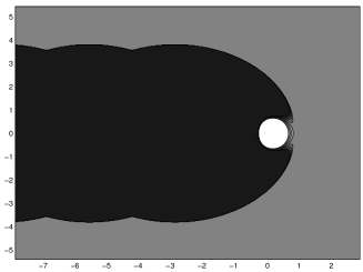
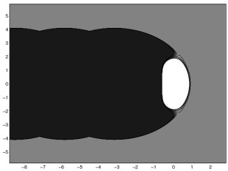
FIG. 1.: Energy contours for monomer approaching fiber tip with hard (a) and soft (b) force fields. Contour heights correspond to integer multiples of $kT$, with lighter corresponding to lower energies. The length units are nm, assuming a monomer step size of 2.7 nm as for actin.

B Filament-Growth Procedure

A typical physiological concentration of actin ($10~{}\mu$M) is low in the sense that the average spacing between actin monomers is about 60 nm, roughly 10 times the monomer size. This means that the probability that two free monomers are near enough to interact with each other is very small. For this reason we adopt a growth procedure in which only one free monomer at at time interacts with the tip. This is accomplished as follows. We start with a fiber of six monomers pointing in the $z$-direction, at their equilibrium spacing. A free monomer is then added at a point on a circle of radius $R$ centered on the next attachment site[18] (defined as one monomer spacing beyond the monomer at the fiber tip). We choose $R=2.5a$, which places the added monomer well beyond the interaction range of the monomer at the tip. The relative probabilities of monomer addition at different points on the circle are proportional to $\exp{[-W_{2}(z)/kT]}$. This weighting is accomplished by choosing a random number for each potential addition point; if this random number is less than $\exp{[-W_{2}(z)/kT]}$, then this point is rejected and another one is chosen. A new point is also chosen if the monomer overlaps the fiber (i.e., its distance to the fiber is less than $r_{\rm max}$). The system is then stepped forward in time according to the procedure described above, until one of two possible termination events occur:

• 1. The monomer diffuses outside of the $R$-circle. In this case it is restarted on the circle as above. If the obstacle abuts the fiber, the position of the monomer is constrained to be out of the interaction range of the obstacle.

• 2. The monomer attaches to the tip. In this case, another monomer is started on the $R$-circle.

In this way, the CPU time that is used in the simulation is focused on the time that the monomers spend close to the tip. A typical snapshot of a simulation configuration is shown in Figure 2.

figure=Fig2.ps,width=3cm,height=3.5cm

FIG. 2.: Typical fiber-obstacle configuration during simulations.

One can use the computed growth rates to predict growth rates for low concentrations $c$, by simply multiplying the computed rates by the probability $P(c)$ of finding a monomer inside the $R$-circle. We obtain this probability numerically as

$$P(c)=\frac{1}{c}\int_{r<R}\exp{(-U(\vec{r})/kT)}d^{2}r~{}~{},$$ (12)

where $U(\vec{r})$ is the energy (from both fiber and obstacle) associated with placing a monomer at the point $\vec{r}$, and the coordinates are given with respect to the next attachment point[19]. We plot our force-velocity relations in terms of the force acting between the obstacle and the fiber tip. This exceeds the external force applied on the obstacle by an amount corresponding to the viscous drag on the obstacle as it moves through the medium. The total force is thus given as $F=F_{\rm ext}+v/\mu_{O}$.

III Results

Our simulations involve 10 runs, each of which involves the addition of 30 monomers to the fiber tip. This corresponds to a statistical uncertainty of $\sqrt{1/300}=6\%$ in the growth velocities. Typical results for the fiber length as a function of time are shown in Figure 3. Note that there are no backwards steps, because the parameters that are used in the force field result in an exothermic enthalpy for monomer addition that exceeds $kT$ by at least a factor of 20. We use a concentration corresponding to one monomer per square of side $20a$; in our model, velocities at other concentrations would be given by a linear proportionality.

FIG. 3.: Representative plot of number of monomers in fiber vs. number of time steps. Obtained for $Fa/kT=1.5$ and hard force field.

A Force-Velocity Relation

Figure 4a shows growth velocity (solid circles) vs. applied force, for the “hard” force field (cf. Figure 1a). For comparison, a curve proportional to $\exp{(-Fa/kT)}$ is shown. The simulation results give noticeably lower velocities at finite applied forces than the exponential prediction. The discrepancy is about $65\%$ at $Fa/kT=1$, and $85\%$ at $Fa/kT=2.5$. The results can be roughly fitted to different exponential curve, of the form $\exp{(-1.7~{}Fa/kT)}$. Thus the growth velocity is much more sensitive to force than the thermal-ratchet model would predict. Figure 4b shows similar results for the soft force field (cf. Figure 1b). The free-fiber growth velocity is about twice that for the “hard” force field, because the attraction basin is larger. The discrepancies between the simulation results and the analytic theory are comparable to those seen for the “hard” force field, but somewhat less pronounced. The discrepancy at $Fa/kT=2.5$ is $70\%$, and the exponential fit curve is $\exp{(-1.5~{}Fa/kT)}$. The open diamonds in Fig. 4b correspond to the results of varying the mobility $\mu_{O}$; for the leftmost one the mobility is doubled, and for the rightmost one it is reduced by a factor of ten. The effects of these variations are very minor, as predicted by the “thermal-ratchet” model[12].

FIG. 4.: Growth rates (solid circles) for hard (a) and soft (b) force fields vs. total force $F$. Rates given in units of $\mu kTc$, where $\mu$ is the monomer mobility and $c$ is the concentration. Force given in units of $a/kT$. Solid line corresponds to exponential decay (cf. Eq. (1)). Diamonds in (a) correspond to mobility enhanced by factor of 2 (left) and reduced by factor of 10 (right). Dashed curves correspond to theory of Eq. (12).

B Interpretation

We believe that the discrepancies seen in Fig. 4 result from the restriction of monomer diffusion to the fiber tip by the impinging obstacle. Such restriction will occur even when the obstacle is elevated by a distance $a$ or more. Figure 5 shows energy contours for a monomer approaching the tip, when the obstacle is elevated a distance $1.25a$ relative to its equilibrium position for $Fa/kT=1.0$. The contours at at integer multiples of $kT$. The easily accessible paths corresponding to energies less than $kT$ are confined to a narrow band by the presence of the obstacle. This is expected to slow the diffusion to the tip. Effectively, the monomers must travel through a tunnel in order to get to the basin of attraction near the tip. Another possible explanation for the observed effect would be that even in the region with energy less than $kT$, there is a finite energy from the interaction with the obstacle. However, this energy is proportional to the the length scale of the interaction between the obstacle and the monomers. In a few cases, we have made this length scale five times smaller, and the velocities are unchanged to within a few percent. Therefore, this monomer-obstacle interaction energy does not seem to be the major factor, but rather the blocking effects of the obstacle.

figure=Fig5.ps,width=4cm,height=3.25cm

FIG. 5.: Energy contours for monomer approaching fiber tip with hard force field, in presence of obstacle. Contours are as in Fig. 1.

To make this physical picture more precise, we have calculated the velocities for model fiber configurations in which the obstacle is held at a fixed distance from the fiber tip. The results are shown in Figs. 6a and b, for the “hard” and “soft” force fields respectively. The distance $Z$ is measured in units of the monomer size, and the edge of the obstacle is defined as the point where the monomer-obstacle interaction energy is equal to $kT$. Thus when $Z=0$, the interaction energy of the last monomer in the fiber with the obstacle is $kT$. In both cases, the velocity at $Z/a=1$ is nearly zero. Only for $Z/a>2$ is the velocity within $20\%$ of the free-growth velocity.

The appropriate generalization of Eq. (1) is then the following:

$$v(F)=\int^{\infty}_{0}v(Z)P(Z,F)dZ~{}~{}~{},$$ (13)

where $F$ is the applied force, $Z$ is the obstacle position, and $P(Z,F)=(\rm const)\exp{(-E/kT)}$ is the probability of a certain value of $Z$. Here the obstacle-fiber interaction energy is $E=W_{2}(z-Z)+FZ$, where $z$ is the z-coordinate of the last monomer in the fiber. Equation (13) reduces to Eq. (1) if $v(Z)$ has the form of a step function beginning at a $Z=a$, and $W_{2}$ is sufficiently short-ranged. The dashed lines in Figs. 4a and 4b correspond to a numerical evaluation of Eq. (13). For both force fields, the agreement with the simulation results is quite close, with only about $20\%$ discrepancies occurring for small but non-zero forces. Thus the gradual rise of the velocity seen in Fig. 6, as opposed to an abrupt jump, is at the heart of the observed effect.

FIG. 6.: Fiber growth velocity with fixed tip-fiber spacing, for hard (a) and soft (b) force fields. $Z$ is measured relative to point at which tip-fiber interaction energy is $kT$.

IV Conclusions

The physics underlying the above results is general enough that in most systems involving fiber growth against an obstacle, one should expect a decay of velocity with applied force more rapid than the simple exponential form (1). This may explain some of the discrepancies pointed out in connection with the measured force-velocity relation of Ref. [11]. However, our application to microtubule growth is not quantitative enough to determined whether the present effect exceeds the subsidy effects discussed in Ref. [16]. The results obtained here should be useful in explaining the basic physics of motion based on actin polymerization. For example, in a recent study van Oudenaarden and Theriot[20] have simulated the propulsion of plastic beads in cell extracts with a model based on a number of fibers exerting forces on the beads. In their simulations, an assumed form is taken for the probability of monomer addition to a fiber in terms of the time-averaged position of the fiber relative to the bead, or equivalently the force acting between the two. A better knowledge of the relationship between the force and the monomer addition rate can help pin down the validity of the assumptions underlying such simulations. Because the bead-motion simulations include only the thermal energy required to achieve a certain tip-obstacle spacing, it is likely that the addition rate will drop off more rapidly with increasing force than is assumed in Ref. [20].

The results obtained here are also expected to have noticeable results on the structure of membranes that are being pushed forward by collections of actin fibers. As a result of random fluctuations, some fibers will eventually get ahead of others, and these will be exerting larger forces on the membrane. If the velocity drops off rapidly with the force, then these fibers will be slowed down significantly. This will result in the membrane surface being smoother than otherwise expected. Future work should treat such many-fiber effects, and also explore the effects of fiber growth angle and branching.

- [1] T. Pollard, J. Cell Biol. 103, 2747 (1986).
- [2] J. A. Cooper, Ann. Rev. Physiol. 53, 585 (1991).
- [3] J.-B. Marchand et al., J. Cell Biol. 130, 331 (1995).
- [4] V. Argiro, M. Bunge, and J. Johnson, J. Neurosci. Res. 13, 149 (1985).
- [5] S. Felder and E. L. Elson, J. Cell Biol. 111, 2513 (1990).
- [6] L. G. Tilney and D. A. Portnoy, J. Cell Biol. 109, 1597 (1989).
- [7] A. S. Sechi, J. Wehland, and J. V. Small, J. Cell Biol. 137, 155 (1997).
- [8] L. A. Cameron, M. J. Footer, A. van Oudenaarden, and J. A. Theriot, Proc. Natl. Acad. Sci. 96, 4908 (1999).
- [9] V. C. Abraham, V. Krisnamurthi, D. L. Taylor, and F. Lanni, Biophys. J. 77, 1721 (1999).
- [10] C. Rotsch, K. Jacobson, and M. Radmacher, Proc. Natl. Acad. Sci. USA 96, 921 (1999).
- [11] M. Dogterom and B. Yurke, Science 278, 856 (1997).
- [12] C. S. Peskin, G. M. Odell, and G. F. Oster, Biophysical Journal 65, 316 (1993).
- [13] T. L. Hill, Linear Aggregation Theory in Cell Biology (Springer-Verlag, New York, 1987), Chap. 2.
- [14] A. Mogilner and G. Oster, Biophys. J. 71, 3030 (1996).
- [15] A. Mogilner and G. Oster, Eur. Biophys. J. 25, 47 (1996).
- [16] A. Mogilner and G. Oster, Eur. Biophys. J. 28, 235 (1999).
- [17] M. Doi and S. F. Edwards, The Theory of Polymer Dynamics (Clarendon Press, Oxford, 1998), Chap. 3.
- [18] In order to avoid an excessive number of excursions back and forth across the circle radius, the added monomer is placed a small distance inside R.
- [19] In two dimensions, the time for a particle to diffuse to capture is not strictly proportional to the area of the region in which it diffuses, but contains logarithmic corrections. Therefore the calculated velocities are not strictly independent of . I have verified by use of a few test cases with larger values of that the predicted logarithmic scaling is observed. Extrapolating to a value of corresponding to a physiological interparticle spacing for actin monomers would modify the calculated velocities by a constant factor of about two, which we have not included because our focus is the force-dependence of the velocity rather than its absolute magnitude.
- [20] A. van Oudenaarden and J. A. Theriot, Nature Cell. Biol. 1, 493 (1999).