Performance of Discrete Heat Engines and Heat Pumps in Finite Time.

Abstract

The performance in finite time of a discrete heat engine with internal friction is analyzed. The working fluid of the engine is composed of an ensemble of noninteracting two level systems. External work is applied by changing the external field and thus the internal energy levels. The friction induces a minimal cycle time. The power output of the engine is optimized with respect to time allocation between the contact time with the hot and cold baths as well as the adiabats. The engine’s performance is also optimized with respect to the external fields. By reversing the cycle of operation a heat pump is constructed. The performance of the engine as a heat pump is also optimized. By varying the time allocation between the adiabats and the contact time with the reservoir a universal behavior can be identified. The optimal performance of the engine when the cold bath is approaching absolute zero is studied. It is found that the optimal cooling rate converges linearly to zero when the temperature approaches absolute zero.

I Introduction

Analysis of heat engines has been a major source of thermodynamic insight. The second law of thermodynamics resulted from Carnot’s study of the reversible heat engine [1]. Study of the endo-reversible Newtonian engine [2] began the field of finite time thermodynamics [3, 4, 5, 6]. Analysis of a virtual heat engine by Szilard led to the connection between thermodynamics and information theory [7, 8]. Recently this connection has been extended to the regime of quantum computation [9].

Quantum models of heat engines show a remarkable similarity to engines obeying macroscopic dynamics. The Carnot efficiency is a well established limit for the efficiency of lasers as well as other quantum engines [10, 11, 12, 13, 14]. Moreover, even the irreversible operation of quantum engines with finite power output has many similarities to macroscopic endo-reversible engines [15, 16, 17, 18, 19].

It is this line of thought that serves as a motivation for a detailed analysis of a discrete four stroke quantum engine. In a previous study [20], the same model served to find the limits of the finite time performance of such an engine but with the emphasis on power optimization. In that study the working medium was composed of discrete level systems with the dynamics governed by a master equation. The purpose was to gain insight into the optimal engine’s performance with respect to time allocation when external parameters such as: the applied fields, the bath temperatures and the relaxation rates were fixed.

The present analysis emphasizes the reverse operation of the heat engine as a heat pump. For an adequate description of this mode of operation inner friction has to be a consideration. Without it the model is deficient with respect to optimizing the cooling power. Another addition is the optimization of the external fields. This is a common practice when cold temperatures are approached. With the addition of these two attributes, the four stroke quantum model is analyzed both as a heat engine and as a refrigerator.

Inner friction is found to have a profound influence on performance of the refrigerator. A direct consequence of the friction is a lower bound on the cycle time. This lower bound excludes the non-realistic global optimization solutions found for frictionless cases [20] where the cooling power can be optimized beyond bounds. This observation, has led to the suggestion of replacing the optimization of the cooling power by the optimization of the cooling efficiency per unit time [21, 22, 23, 24]. Including friction is therefore essential for more realistic models of heat engines and refrigerators with the natural optimization goal becomes either the power output or the cooling power. The source of friction is not considered explicitly in the present model. Physically friction is the result of non-adiabatic phenomena which are the result of the rapid change in the energy level structure of the system. For example friction can be caused by the missalignement of the external fields with the internal polarization of the working medium. For a more explicit description of the friction the interactions between the individual particles composing the working fluid have to be considered. The present model is a microscopic analogue of the Ericsson refrigeration cycle [25] where the working fluid consists of magnetic salts. The advantage of the microscopic model is that the use of the phenomenological heat transfer laws can be avoided [16]. The results of the present model are compared to a recent analysis of macroscopic chillers [27]. In that study, a universal modeling was demonstrated. It is found that the discrete quantum version of heat pumps has behavior similar to that of macroscopic chillers.

There is a growing interest in the topic of cooling atoms and molecules to temperatures very close to absolute zero [28]. Most of the analysis of the cooling schemes employed are based on quantum dynamical models. New insight can be gained by employing a thermodynamic perspective. In particular the temperatures achieved are so low that the third law of thermodynamics has to be considered. The discrete level heat pump can serve as a model to study the third law limitations. The finite time perspective of the third law is a statement on the asymptotic rate of cooling as the absolute temperature is approached. These restrictions are imposed on the optimal cooling rate. The behavior of the optimal cooling rate as the absolute temperature is approached is a third law upper bound on the cooling rate. The main finding of this paper is that the optimal cooling rate converges to zero linearly with temperature, and the entropy production reaches a constant when the cold bath temperature approaches absolute zero.

II Basic Assumptions and Formal Background for the Heat Engine and the Heat Pump

Heat engines and heat pumps are characterized by three attributes: the working medium, the cycle of operation, and the dynamics which govern the cycle. Heat baths by definition are large enough so that their temperatures is constant during the cycle of operation. The heat engine and the heat pump are constructed from the same components and differ only by their cycle of operation.

A The Working Medium

The working medium consists of an ideal ensemble of many non-interacting discrete level systems. Specifically, the analysis is carried out on two-level systems (TLS) but an ensemble of harmonic oscillators [20] would lead to equivalent results.

The TLS systems are envisioned as spin-1/2 systems. The lack of spin-spin interactions enables the description of the energy exchange between the working medium and the surroundings in terms of a single TLS. The state of the system is then defined by the average occupation probabilities $P_{+}$ and $P_{-}$ corresponding to the energies ${1\over 2}\omega$ and $-{1\over 2}\omega$, where $\omega$ is the energy gap between the two levels. The average energy per spin is given by

$$E={P_{+}}\cdot\left({1\over 2}\omega\right)+{P_{-}}\cdot\left(-{1\over 2}\omega\right)$$ (1)

The polarization, $S$, is defined by

$$S~{}=~{}{1\over 2}(P_{+}~{}-~{}P_{-})~{}~{}~{},$$ (2)

and thus the energy can be written as $E=\omega S$. Energy change of the working medium can occur either by population transfer from one level to the other (changing S) or by changing the energy gap between the two levels (changing $\omega$). Hence

$$dE~{}=~{}Sd\omega~{}+~{}\omega dS~{}~{}.$$ (3)

Population transfer is the microscopic realization of heat exchange. The energy change due to external field variation is associated with work. Eq. (3) is therefore the first law of thermodynamics:

$$D{\cal W}~{}\equiv~{}Sd\omega~{}~{};~{}~{}D{\cal Q}~{}\equiv~{}\omega dS~{}~{}.$$ (4)

Finally, for TLS the internal temperature, $T^{\prime}$, is always defined via the relation

$$S~{}=~{}-{1\over 2}\tanh\left({{\omega}\over{2k_{B}T^{\prime}}}\right)~{}~{}.$$ (5)

Note that the polarization $S$ is negative as long as the temperature is positive.

B The Cycle of Operation

1 Heat engines cycle

The cycle of operation is analyzed in terms of the polarization and frequency $(S,\omega)$. A schematic display is shown in Fig.(1) for a constant total cycle time, $\tau$. The present engine is an irreversible four stroke engine [20] resembling the Stirling cycle, with the addition of internal friction. The direction of motion along the cycle is chosen such that net positive work is produced.

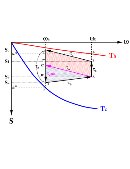
FIG. 1.: The heat engine with friction in the $\omega$ ,$S$ plane. $T_{h}$ is the hot bath temperature. $\tau_{h}$ is the time allocation when in contact with the hot bath. $T_{c}$ and $\tau_{c}$ represent the temperature and time allocation for the cold bath. $\tau_{a}$ represents the time allocation for compression (field change from $\omega_{b}$ to $\omega_{a}$) and $\tau_{b}$ for expansion. The area  A,B, C¹, D¹ is the positive work done by the system, while the areas  C, C¹, S₁, S₃, and D¹, D, S₄, S₂ represent the negative work done by the system.

The four branches of the engine will be now briefly described.

On the first branch, $A\rightarrow B$, the working medium is coupled to the hot bath of temperature $T_{h}$ for period $\tau_{h}$, while the energy gap is kept fixed at the value $\omega_{b}$. The conditions are such that the internal temperature of the medium is lower than $T_{h}$. In this branch, the polarization is changing from the initial polarization $S_{2}$ to the polarization $S_{1}$. The inequality to be fulfilled is therefore:

$$S_{1}<~{}-{1\over 2}\tanh\left({{\omega_{b}}\over{2k_{B}T_{h}}}\right)~{}~{}.$$ (6)

Since $\omega$ is kept fixed, no work is done and the only energy transfer is the heat $\omega_{b}(S_{1}-S_{2})$ absorbed by the working medium.

In the second branch, $B\rightarrow C$ the working medium is decoupled from the hot bath for a period $\tau_{a}$, and the energy gap is varied linearly in time, from $\omega_{b}$ to $\omega_{a}$. In this branch work is done to overcome the inner friction which develops heat, causing the polarization to increase from $S_{1}$ to $S_{3}$ (Cf. Fig. 1). The change of the internal temperature is the result of two opposite contributes. First lowering the energy gap leads to a lower inner temperature for constant polarization $S$. Second increase in polarization due to friction, leads to an increase of the inner temperature for fixed $\omega$. The inner temperature $T^{\prime}$ at point C might therefore be lower or higher than the initial temperature at point B.

The third branch $C\rightarrow D$, is similar to the first. The working medium is now coupled to a cold bath at temperature $T_{c}$ for time $\tau_{c}$. The polarization changes on this branch from $S_{3}$ to the polarization $S_{4}$. For the cycle to close, $S_{4}$ should be lower than $S_{2}$. At the end of the cycle the internal temperature of the working medium should be higher than the cold bath temperature, $T^{\prime}>{T_{c}}$, leading to:

$$S_{4}~{}>~{}-{1\over 2}\tanh\left({{\omega}_{a}\over{2k_{B}T_{c}}}\right)~{}~{}.$$ (7)

Since $S_{4}<S_{1}$ (Fig. 1), it follows from Eq. ( 6) and Eq.( 7), that:

$$\left(\omega_{a}\over T_{c}\right)~{}>~{}\left(\omega_{b}\over T_{h}\right)$$ (8)

Inequality (8) is equivalent to the Carnot efficiency bound, from Eq. (8) one gets:

$$1~{}~{}-~{}~{}\left(\omega_{a}\over\omega_{b}\right)~{}<~{}1~{}~{}-~{}~{}\left(T_{c}\over T_{h}\right)~{}=~{}\eta_{Carnot}$$ (9)

The present model is a quantum analogue of the Stirling engine which also has Carnot’s efficiency as an upper bound.

The polarization $S$ changes uni-directionally along the ’adiabats’ due to the increase of the excited level population as a result of the heat developed in the working fluid when work is done against friction, irrespective of the direction of the field change.

The fourth branch $D\rightarrow A$, closes the cycle and is similar to the second. The working medium is decoupled from the cold bath. In a period $\tau_{b}$ the energy gap is changing back to its original value, $\omega_{b}$. The polarization increases from $S_{4}$ to the original value $S_{2}$.

TABLE I.: Work and heat exchange along the branches of the heat engine with friction

branch	work+[work against friction]	heat
$A\rightarrow B$	$0$	$\omega_{b}(S_{1}-S_{2})$
$B\rightarrow C$	$(\omega_{a}-\omega_{b})(S_{1}+\sigma^{2}/(2\tau_{a}))$  +  [ $\sigma^{2}(\omega_{a}+\omega_{b})/(2\tau_{a})$ ]	$0$
$C\rightarrow D$	$0$	$\omega_{a}((S_{2}-S_{1})-\sigma^{2}(1/\tau_{a}+1/\tau_{b}))$
$D\rightarrow A$	$(\omega_{b}-\omega_{a})(S_{2}-\sigma^{2}/(2\tau_{b}))$  +  [ $\sigma^{2}(\omega_{a}+\omega_{b})/(2\tau_{b})$ ]	$0$

2 Refrigerator cycle

The purpose of a heat pump is to remove heat from the cold reservoir by employing external work. The cycles of operation in the $(S,\omega)$ plane is schematically shown in Fig. 2,

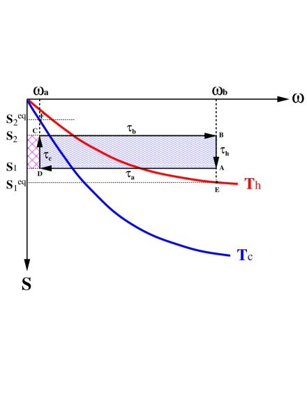
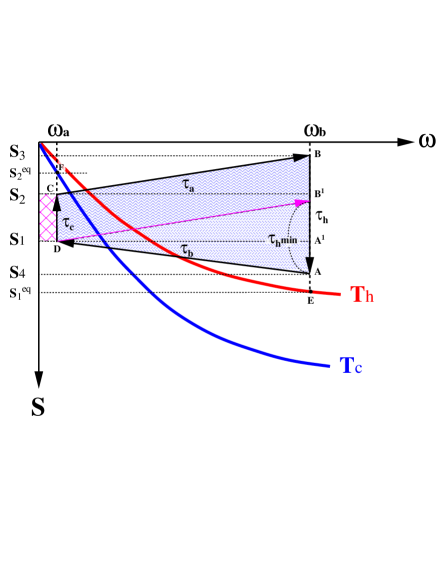
FIG. 2.: The cycle of operation of the heat pump. Left: without friction. S${}_{1}^{eq}$ is the hot bath equilibrium polarization. S${}_{2}^{eq}$ is the cold bath equilibrium polarization. The area enclosed by D,C,S₂ S₁ is the heat absorbed form the cold bath. The area enclosed by DCBA is the work done on the system. Right: with friction. The area enclosed by D,C,S₂,S₁ is the heat absorbed form the cold bath. The work on the system is the area defined by the rectangles B B¹ S₂ S₃ and B¹ A¹ D C and A¹ A S₄ S₁.

The cycle of operation resembles the Ericsson refrigeration cycle [25]. The differences are in the dynamics of the microscopic working fluid which are described in subsection II C. The work and heat transfer for the heat pump is summarized in Table II.

The four branches for the heat pump become:

In the first branch, $D\rightarrow C$, the working medium is coupled to the cold bath of temperature $T_{c}$ for time $\tau_{c}$, while the energy gap is kept fixed at the value $\omega_{a}$. The conditions are such that the internal temperature of the medium is lower than $T_{c}$ during $\tau_{c}$. Along this branch, the polarization changes from the initial polarization $S_{1}$ to the polarization $S_{2}$. Since $\omega$ is kept fixed, no work is done and the only energy transfer is the heat $\omega_{a}(S_{2}-S_{1})$ absorbed by the working medium. On this branch:

$$S_{2}<~{}-{1\over 2}\tanh\left({{\omega_{a}}\over{2k_{B}T_{c}}}\right)~{}~{}.$$ (10)

In the second branch, $C\rightarrow B$ the working medium is decoupled from the cold bath, and the energy gap is varied. In the frictionless case the polarization $S_{2}$ is constant (Left of Fig. 2). The only energy exchange is the work done on the system ( Table II). When friction is added the polarization is changing from $S_{2}$ to $S_{3}$ in a period $\tau_{a}$. The energy gap changes from $\omega_{a}$ to $\omega_{b}$ (Right of Fig. 2), according to a linear law. In addition to work, heat is developing as a result of the inner friction ( Table II).

The third branch $B\rightarrow A$, is similar to the first. The working medium is coupled to the hot bath at temperature $T_{h}$, for time $\tau_{h}$, keeping the energy gap $\omega_{b}$ fixed. In this branch the polarization changes from $S_{2}$ to $S_{1}$ in the frictionless case, and from $S_{3}$ to $S_{4}$ when friction is added. The constraint is that the internal temperature of the working medium should be higher than the hot bath temperature during the time $\tau_{h}$, $T^{\prime}>T_{h}$, leading to the inequality (Fig. 2),

$$S_{1}>~{}S_{4}~{}>~{}~{}-{1\over 2}\tanh\left({{\omega_{b}}\over{2k_{B}T_{h}}}\right)~{}~{}.$$ (11)

therefore $S_{2}>S_{1}$. From Eqs. (10) and (11), the condition for the interrelation between the bath temperatures and the field values becomes:

$$\left(\omega_{a}\over T_{c}\right)~{}<~{}\left(\omega_{b}\over T_{h}\right)$$ (12)

which is just the opposite inequality of the heat engine, (Eq. 8). In the heat pump work is done on the working fluid and since no useful work is done Carnot’s bound is not violated.

The fourth branch $A\rightarrow D$, closes the cycle and is similar to the second. The working medium is decoupled from the cold bath, and the energy gap changes back, during a period $\tau_{b}$ to its original value, $\omega_{b}$.

The results are summarized in Table II.

TABLE II.: Work and heat exchange along the branches of the heat pump without/with friction.

branch	frictionless work/work+[work against friction]	heat
D$\rightarrow$C	0	$\omega_{a}(S_{2}-S_{1})$
C$\rightarrow$B	$\begin{array}[]{c}(\omega_{b}-\omega_{a})S_{2}\\ \left(\omega_{b}-\omega_{a})(S_{2}+\sigma^{2}/(2\tau_{a})\right)+[\sigma^{2}(\omega_{a}+\omega_{b})/(2\tau_{a})]\\ \\ \end{array}$	0
B$\rightarrow$A	0	$\begin{array}[]{c}\omega_{b}(S_{1}-S_{2})\\ \omega_{b}\left((S_{1}-S_{2})-\sigma^{2}(1/\tau_{a}+1/\tau_{b})\right)\\ \end{array}$
A$\rightarrow$D	$\begin{array}[]{c}(\omega_{a}-\omega_{b})S_{1}\\ (\omega_{a}-\omega_{b})\left(S_{1}-\sigma^{2}/(2\tau_{b})\right)+[\sigma^{2}(\omega_{a}+\omega_{b})/(2\tau_{b})]\\ \\ \end{array}$	0

C Dynamics of the working medium

The dynamics of the system along the heat exchange branches is represented by changes in the level population of the two-level-system. This is a reduced description in which the dynamical response of the bath is cast in kinetic terms [18]. Since the dynamics has been described previously [20] only a brief summary of the main points is presented here, emphasizing the differences in the energy exchanges on the ’adiabats’.

1 The dynamics of the heat exchange branches

The dynamics of the population at the two levels, $P_{+}$ and $P_{-}$, are described via a master equation

$$\left\{\begin{array}[]{l}{{{dP_{+}}\over{dt}}=-k_{\downarrow}P_{+}~{}+~{}k_{\uparrow}P_{-}}\\ {{{dP_{-}}\over{dt}}=~{}k_{\downarrow}P_{+}~{}-~{}k_{\uparrow}P_{-}}\end{array}\right.~{}~{},$$ (15)

where $k_{\downarrow}$ and $k_{\uparrow}$ are the transition rates from the upper to the lower level and vice versa. The explicit form of these coefficients depend on the nature of the bath and the system bath coupling interactions. The thermodynamics partition between system and bath is consistent with a weak coupling assumption [18]. Temperature enters through detailed balance. The equation of motion for the polarization $S$ obtained from Eq. (15) becomes:

$${{dS}\over{dt}}~{}=~{}-\Gamma(S~{}-~{}S^{eq})~{}~{}$$ (16)

where

$$\Gamma~{}=~{}{k_{\downarrow}}~{}+~{}{k_{\uparrow}}$$ (17)

and

$$S^{eq}~{}=~{}-{1\over 2}{{{k_{\downarrow}}~{}-~{}{k_{\uparrow}}}\over{{k_{\downarrow}}~{}+~{}{k_{\uparrow}}}}=-{1\over 2}\tanh\left({\omega\over{2k_{B}T}}\right)~{}~{}$$ (18)

where $S^{eq}$ is the corresponding equilibrium polarization. It should be noticed that in a TLS there is a one to one correspondence between temperature and polarization thus internal temperature is well defined even for non-equilibrium situations.

The general solution of Eq (16) is,

$$S(t)~{}=~{}S^{eq}~{}+~{}(S(0)~{}-~{}S^{eq})e^{-\Gamma t}~{}~{}.$$ (19)

where S(0) is the polarization at the beginning of the branch.

From Eqs. (16) and (18) the rate of heat change becomes:

$$\dot{\cal Q}~{}~{}=~{}~{}\omega\dot{S}$$ (20)

See also [16].

For convenience, new time variables are defined:

$$x~{}=~{}e^{-\Gamma_{c}\tau_{c}}~{}~{},~{}~{}y~{}=~{}e^{-\Gamma_{h}\tau_{h}}$$ (21)

These expressions represent a nonlinear mapping of the time allocated to the hot and cold branches by the heat conductivity $\Gamma$. As a result, the time allocation and the heat conductivity parameter become dependent on each other.

Figure 1 and 2 show that the friction induces an asymmetry between the time allocated to the hot and cold branches since more heat has to be dissipated on the cold branch.

2 The dynamics on the ’adiabats’

The external field $\omega$ and its rate of change $\dot{\omega}$ are control parameters of the engine. For simplicity it is assumed that the field changes linearly with time:

$${\omega}(t)~{}~{}=~{}~{}\dot{\omega}t~{}~{}+~{}~{}\omega(0)$$ (22)

Rapid change in the field causes non-adiabatic behavior which to lowest order is proportional to the rate of change $\dot{\omega}$. In this context non-adiabatic is understood in its quantum mechanical meaning. Any realistic assumption beyond the ideal non-interacting TLS will lead to such non-adiabatic behavior. It is therefore assumed that the phenomena can be described by a friction coefficient $\sigma$ which forces a constant speed polarization change $\dot{S}$:

$$\dot{S}~{}~{}=~{}~{}\left({\sigma}\over{t^{\prime}}\right)^{2}$$ (23)

where $t^{\prime}$ is the time allocated to the corresponding ’adiabat’. Therefore, the polarization as a function of time becomes:

$$S(t)~{}~{}=~{}~{}S(0)~{}~{}+~{}~{}\left({\sigma}\over{t^{\prime}}\right)^{2}t$$ (24)

where $t\geq 0$ , $t\leq t^{\prime}$. A modeling assumption of internally dissipative friction, similar to Eq.(23), was also made by Gordon and Huleihil ([26]). Friction does not operate on the heat-exchange branches, there is no nonadiabtic effect since the fields $\omega_{a}$ and $\omega_{b}$ are constant in time. The irreversibilities on those branches are due to the transition rates ($\Gamma$) of the master equation.

From Fig.(1), Eq. (4), and Eq. (24) the polarization, for the $B\rightarrow C$ branch of the heat engine becomes:

$$S_{C}=S_{3}~{}~{}=~{}~{}S_{1}~{}~{}+~{}~{}\left({\sigma^{2}}\over{\tau_{a}}~{}\right)~{}.$$ (25)

The work done on this branch is:

$${\cal W}_{BC}~{}=~{}\int_{0}^{\tau_{a}}D{\cal W}~{}=~{}\int_{0}^{\tau_{a}}{S\dot{\omega}dt}~{}~{}=~{}{(\omega_{a}~{}-~{}\omega_{b})}\left(S_{1}~{}+~{}{1\over 2}\left({\sigma}^{2}\over{\tau_{a}}\right)\right)$$ (26)

The heat generated on this branch in the working fluid, which is the work against the friction, becomes:

$${\cal Q}_{BC}~{}=~{}\int_{0}^{\tau_{a}}D{\cal Q}~{}=~{}\int_{0}^{\tau_{a}}{\omega\dot{S}dt}~{}~{}=~{}{\sigma^{2}(\omega_{a}+\omega_{b})\over{2\tau_{a}}}$$ (27)

This work is dependent on the friction coefficient and inversely on the time allocated to the ’adiabats’. The computation for the other branches of the heat engine and heat pump are similar.

3 Explicit expressions for the polarizations imposed by the closing of the cycle.

By forcing the cycle to close, the four corners of the cycle observed in Fig. 1 are linked. Applying Eq. (19) leads to the equations:

$$\begin{array}[]{l}S_{1}~{}=~{}S_{2}y~{}+~{}S_{h}^{eq}(1-y)\\ S_{3}~{}=~{}S_{1}~{}+~{}{\sigma^{2}\over\tau_{a}}\\ S_{4}~{}=~{}S_{3}x~{}+~{}S_{c}^{eq}(1-x)\\ S_{2}~{}=~{}S_{4}~{}+~{}{\sigma^{2}\over\tau_{b}}\end{array}$$ (32)

The solutions for $S_{1}$, $S_{2}$ and $S_{1}-S_{2}$ are

$$\begin{array}[]{l}S_{1}=S_{c}^{eq}~{}+~{}{\Delta S^{eq}(1-y)~{}+~{}\sigma^{2}yG(x)\over(1-xy)}~{}~{}=~{}~{}S_{h}^{eq}~{}-~{}{\Delta S^{eq}y(1-x)~{}-~{}\sigma^{2}yG(x)\over(1-xy)}\\ S_{2}=S_{c}^{eq}~{}+~{}{\Delta S^{eq}x(1-y)~{}+~{}\sigma^{2}G(x)\over(1-xy)}~{}~{}=~{}~{}S_{h}^{eq}~{}-~{}{\Delta S^{eq}(1-x)~{}-~{}\sigma^{2}G(x)\over(1-xy)}\end{array}$$ (35)

and

$$S_{1}-S_{2}=(\Delta S^{eq})F(x,y)~{}-~{}{\sigma^{2}(1-y)G(x)\over(1-xy)}$$ (36)

where

$$F(x,y)={(1-x)(1-y)\over(1-xy)}~{}~{}~{},~{}~{}~{}\Delta S^{eq}~{}~{}=~{}~{}(S_{h}^{eq}-S_{c}^{eq})~{}~{}~{},~{}~{}~{}G(x)~{}=~{}(x/\tau_{a}+1/\tau_{b})$$ (37)

The constraint that the cycle must close leads to conditions on the polarizations $S_{1}$ and $S_{2}$ and on the minimum cycle time $\tau_{c,min}$. Eqs. (35) shows that both $S_{1}$ and $S_{2}$ are bounded by $S_{h}^{eq}$ and $S_{c}^{eq}$. The minimum cycle time is obtained when the polarizations coincide with the hot bath polarization: $S_{1}$=$S_{2}$=$S_{h}^{eq}$. In this case, $\tau_{h}$=0, and from Eqs. (21) and (36) the minimum time allocation on the cold bath $\tau_{c,min}$ is computed,

$$x_{max}~{}=~{}{(S_{h}^{eq}-S_{c}^{eq})~{}-~{}{\sigma^{2}/\tau_{b}}\over(S_{h}^{eq}-S_{c}^{eq})~{}+~{}{\sigma^{2}/\tau_{a}}}$$ (38)

or

$$\tau_{c,min}~{}=~{}-{1/\Gamma_{c}}\lg{(S_{h}^{eq}-S_{c}^{eq})~{}-~{}{\sigma^{2}/\tau_{b}}\over{(S_{h}^{eq}-S_{c}^{eq})~{}+~{}{\sigma^{2}/\tau_{a}}}}$$ (39)

From this expression for $\tau_{c,min}$ the lower bound for the overall cycle time, is obtained (The left of Fig. 3) :

$$\tau~{}\geq~{}\tau_{min}~{}=~{}\tau_{c,min}+\tau_{a}+\tau_{b}$$ (40)

When the minimum cycle time Eq. (39) diverges, the cycle cannot be closed. This condition imposes an upper bound on the friction coefficient $\sigma$

$$\sigma~{}~{}\leq~{}~{}\sigma^{up}~{}=~{}\sqrt{~{}\tau_{b}(S_{h}^{eq}-S_{c}^{eq})}.$$ (41)

or

$$~{}\tau_{b}>\tau_{b,min}~{}=~{}{\sigma^{2}\over(S_{h}^{eq}-S_{c}^{eq})}.$$ (42)

Closing of the cycle imposes similar constraints on the minimal cycle time under friction for the heat pump. The value of the polarization difference $S_{2}-S_{1}$ using the notation of Fig. 2 becomes:

$$S_{2}-S_{1}=(S_{2}^{eq}-S_{1}^{eq})F(x,y)~{}-~{}{\sigma^{2}(1-x)(y/\tau_{a}+1/\tau_{b})\over(1-xy)}$$ (43)

The minimum cycle time is calculated in the limit when $\tau_{c}$=0, leading to $S_{2}$=$S_{1}$=$S_{2}^{eq}$. From Eqs. (21) and (43) the minimum time allocation on the hot branch $\tau_{h,min}$ is computed:

$$y_{max}~{}=~{}{(S_{2}^{eq}-S_{1}^{eq})~{}-~{}{\sigma^{2}/\tau_{b}}\over(S_{2}^{eq}-S_{1}^{eq})~{}+~{}{\sigma^{2}/\tau_{a}}}$$ (44)

$$\tau_{h,min}~{}=~{}-{1/\Gamma_{h}}\lg{(S_{2}^{eq}-S_{1}^{eq})~{}-~{}{\sigma^{2}/\tau_{b}}\over{(S_{2}^{eq}-S_{1}^{eq})~{}+~{}{\sigma^{2}/\tau_{a}}}},$$ (45)

where $S_{2}^{eq}$ is point F and $S_{1}^{eq}$ is point E on Fig. 2. Using $\tau_{h,min}$ the lower bound for the overall cycle time, is computed

$$\tau~{}\geq~{}\tau_{min}~{}=~{}\tau_{h,min}+\tau_{a}+\tau_{b}$$ (46)

Closing the cycle imposes a minimum cycle time for both the heat engine and the heat pump, which is a monotonically increasing function of the friction coefficient $\sigma$. The divergence of $\tau_{min}$ imposes a maximum value for the friction coefficient $\sigma$.

D Finite Time Analysis

1 Quantities to be Optimized.

The primary variable to be optimized is the power of the heat engine and the heat-flow extracted from the cold reservoir of the heat pump. For a preset cycle time, optimization of the power is equivalent to optimization of the total work, while optimization of heat flow is equivalent to the optimization of the heat absorbed. The entropy production will also be analyzed.

(1) The total work done on the environment per cycle of the Heat Engine.

The total work of the engine, is the sum of the work on each branch: Cf. (Table I and Fig. 1):

$${\cal W}_{cyle1}~{}=~{}\oint D{\cal W}~{}=~{}-\left(W_{AB}+W_{BC}+W_{CD}+W_{DA}\right)$$ (47)

which becomes:

$${\cal W}_{cyle1}~{}=~{}(\omega_{b}-\omega_{a})(S_{1}-S_{2})~{}-~{}\sigma^{2}\omega_{a}(1/\tau_{a}~{}+~{}1/\tau_{b})$$ (48)

The negative sign is due to the convention of positive ${\cal W}$ when work is done on the system.

Analyzing Eq. (48), the work is partitioned into three positive and negative areas. The positive area (left rotation)

$${\cal W}_{p}~{}=~{}(\omega_{b}-\omega_{a})(S_{1}-S_{2})$$ (49)

is defined by the points $A,B,C^{1},D^{1}$ in Fig. 1. The two negative areas (right rotation)

$${\cal W}_{n}~{}=~{}\sigma^{2}\omega_{a}(1/\tau_{a})~{}~{}+~{}~{}\sigma^{2}\omega_{a}(1/\tau_{b})$$ (50)

are defined by the points $C,C^{1},S_{1},S_{3}$ and $D^{1},D,S_{4},S_{2}$ in Fig. 1.

The cycle which achieves the minimum cycle time $\tau$ = $\tau_{c,min}$, produces zero positive work ${\cal W}_{p}=0$. The corners A and B coincide at E, and $C^{1}$ coincides with $D^{1}$. The negative work of Eq. (50), is defined by the corners $C,D,S_{4},S_{3}$ and is ’cut’ by the $S_{h}^{eq}$ line (Cf. the right of Fig. 4). The cycle has negative total work, meaning that work is done on the working fluid against friction. When $\tau$ increases beyond  $\tau_{c,min}$ , $S_{1}$ diverts from $S_{2}$, becoming lower than $S_{h}^{eq}$   (Cf.Eq. (35)). At a certain point, the work done against friction is exactly balanced by the useful work of the engine. The minimum time in which this balance is achieved is designated $\tau_{0}$. Its value which can be deduced from Eq. (48) is worked out in appendix B.

The minimum cycle time $\tau_{min}$ is compared to $\tau_{0}$, the minimum time needed to obtain positive power shown in the right of Fig. 3 as a function of the friction $\sigma$. Both functions increase with friction, but $\tau_{0}$ diverges at a much lower friction parameter. Above this friction parameter no useful work can be obtained from the engine. The divergence of $\tau_{min}$ corresponds to a larger friction value where the cycle cannot be closed.

FIG. 3.: Left: Minimal cycle time $\tau_{min}$ as a function of the inner friction parameter $\sigma$ for the heat engine. The vertical line represents the upper-bound of $\sigma$. Dimensionless units are used in which $k_{b}=1$ and $\hbar=1$. The parameters used are: $\omega_{a}=1794$, $\omega_{b}=4238$, $T_{c}=500$, $T_{h}=2500$, $\Gamma_{c}=1$ and $\Gamma_{h}=2$. Right: Comparison between $\tau_{min}$ and $\tau_{0}$, the minimum cycle time for power production.

When the total time allocation is sufficient, i.e. $\tau~{}>~{}\tau_{0}$, work is done on the environment, and $S_{1}$ starts to increase. For long cycle times $S_{1}$ will approach $S_{h}^{eq}$, while $S_{2}$ will approach $S_{c}^{eq}$. The constant negative area will become negligible in comparison to the positive area ( Fig. 5).

To study the influence of friction on the work output the polarization difference from Eq. (36) S₁-S₂ is inserted into the work expression Eq. (48), leading to:

$${\cal W}_{cyle1}~{}=~{}(\omega_{b}-\omega_{a})(S_{h}^{eq}-S_{c}^{eq})F(x,y)~{}-~{}{\cal W}_{\sigma 1}$$ (51)

where

$${\cal W}_{\sigma 1}~{}=~{}\sigma^{2}\left({{\omega_{b}(1-y)}(x/\tau_{a}~{}+~{}1/\tau_{b})\over{1-xy}}~{}+~{}{{\omega_{a}(1-x)}(1/\tau_{a}~{}+~{}y/\tau_{b})\over{1-xy}}\right)$$ (52)

${\cal W}_{\sigma 1}$ is the additional ’cost’ due to friction and is always positive.

The emergence of positive power $\cal P$ is shown in Fig. 4. For a fixed cycle time the optimization of work is equivalent to the optimization of power.

The first two cycles have a cycle time shorter than $\tau_{0}$, and therefore do not produce useful work. For cycle 3, $\tau>\tau_{0}$ and positive work is obtained when the time allocation on the cold bath is sufficient $\tau_{c}~{}\geq~{}0.08$.

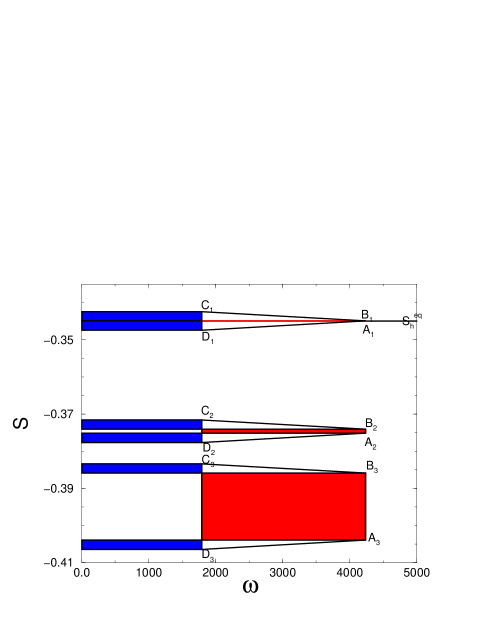
FIG. 4.: Left: Power as a function of the time allocation on the cold branch corresponding to the friction coefficient $\sigma=0.005$ with changing cycle times. The cycle time values are: for curve 1, $\tau$ = $\tau_{min}$ =0.059, for curve 2, $\tau=0.1$ (the first two plots overlap) and for curve 3, $\tau=0.5$. Other parameters are the same as in figure 3. The dashed horizontal line is the line of zero power. Right: The cycles corresponding to the power plots. Negative work is in blue and positive work is in red. Note that for cycles 1 and 2, the total area is negative and, therefore, the power output is negative.

For longer total cycle times, the ratio between the negative area to the positive area decreases as can be seen in Fig. 5.

The position of the cycles in the $S$, $\omega$ coordinates relative to $S_{h}^{eq}$ and $S_{c}^{eq}$ changes as a function of the cycle time. Insight to the origin of the behavior of the ’moving’ cycles is presented in Fig. 11 of Appendix A.

FIG. 5.: Left: Power as a function of the time allocation on the cold branch corresponding to the friction coefficient $\sigma=0.005$ with changing cycle times. The cycle time values are: for curve 4, $\tau=1$, for curve 5, $\tau=2$ and for curve 6, $\tau=5$. The dashed horizontal line is the line of zero power. Right: The cycles corresponding to the power plots. All the constant parameters are as in Fig. 4

The calculation of the total work done on the working fluid per cycle, ${\cal W}^{on}_{cycle3}$ for the heat pump is described in appendix D. See also ( Cf. Table (II) and Cf. Fig. 2).

(2) The heat-flow(${\cal Q}_{F}$)

The heat-flow, ${\cal Q}_{F}$, extracted from the cold reservoir is:

$$~{}~{}~{}{\cal Q}_{F}~{}~{}~{}=\omega_{a}(S_{2}-S_{1})/\tau$$ (53)

Due to the dependence of ${\cal Q}_{F}$ only on $S_{2}$-$S_{1}$, the cycle is similar to the cycle of the heat engine.

(3) The entropy production ($\Delta{\cal S}^{u}$).

The entropy production of the universe, $\Delta{\cal S}^{u}$, is concentrated on the boundaries with the baths since, for a closed cycle, the entropy of the working fluid is constant. The computational details for both the heat engine and the heat pump are shown in appendix C. The entropy production and the power have a reciprocal relation (See Fig. 12). For example, the entropy production increases with $\sigma$, while the power decreases.

(4) Efficiency.

The efficiency of the heat engine is the ratio of useful work to the heat extracted from the hot bath.

$${\eta}_{H.E.}~{}=~{}~{}{{{\cal W}_{cycle}}\over{{\cal Q}_{absorbed}}}~{}~{}=~{}~{}\eta^{fricles}_{H.E.}~{}~{}-~{}~{}\left({{\sigma^{2}\omega_{a}(1/\tau_{a}+1/\tau_{b})}\over\omega_{b}(S_{1}~{}-~{}S_{2})}\right)$$ (54)

where $\eta^{fricles}_{H.E.}~{}=~{}~{}{(1~{}-~{}{\omega_{a}/\omega_{b}})}$

When the cycle time approaches its minimum ${\tau}~{}~{}\rightarrow~{}~{}{\tau_{min}},$ the efficiency diverges: $~{}~{}{\eta}_{H.E.}~{}~{}{\longrightarrow}~{}~{}-~{}{\infty}$. The efficiency becomes positive only when ${\tau}~{}~{}\geq~{}~{}{\tau_{0}}$. Using Eq. (54) a bound for the efficiency is obtained:

$$0~{}~{}<~{}~{}{\eta}_{H.E.}~{}~{}\leq~{}~{}{\eta^{fricles}_{H.E.}~{}~{}-{T_{c}\over{T_{h}}}}\left({{~{}~{}\sigma^{2}(1/\tau_{a}+1/\tau_{b})}\over(S_{1}~{}-~{}S_{2})}\right)$$ (55)

The cooling efficiency of the refrigerator will be:

$${\eta}_{Rf}~{}=~{}~{}{{\cal Q}_{DC}\over{\cal W}_{cycle}^{on}}~{}=~{}{\omega_{a}(S_{2}-S_{1})\over\left((\omega_{b}-\omega_{a})(S_{2}-S_{1})~{}+~{}\sigma^{2}\omega_{b}(1/\tau_{a}+1/\tau_{b})\right)}$$ (56)

or:

$${1\over\eta_{Rf}}+1~{}=~{}{1\over COP}+1~{}=~{}{\omega_{b}\over\omega_{a}}\left(1+{\sigma^{2}(1/\tau_{a}+1/\tau_{b})\over{(S_{2}-S_{1})}}\right)~{}>~{}{T_{h}\over T_{c}}\left(1+{\sigma^{2}(1/\tau_{a}+1/\tau_{b})\over{(S_{2}-S_{1})}}\right)~{}~{}~{}~{}~{},$$ (57)

leading to the expression for the efficiency:

$${\eta}_{Rf}~{}=~{}~{}{\omega_{a}\over\omega_{b}}{1\over{\eta^{fricles}_{H.E.}~{}+~{}{\sigma^{2}(1/\tau_{a}~{}+~{}1/\tau_{b})\over{S_{2}-S_{1}}}}}~{}<~{}{T_{c}\over T_{h}}{1\over{\eta^{fricles}_{H.E.}~{}+~{}{\sigma^{2}(1/\tau_{a}~{}+~{}1/\tau_{b})\over{S_{2}-S_{1}}}}}$$ (58)

For both the heat engine and the heat pump, the efficiency is explicitly dependent on time allocation, cycle time, and bath temperatures.

2 Optimization

The performance of both the heat engine and the heat pump can be optimized with respect to:

• (a) The overall time period $\tau$ of the cycle, and its allocation between the hot and cold branches.

• (b) The overall optimal time allocation between all branches. (This optimization is performed only for the heat pump.)

• (c) The external fields, ($\omega_{a}$, $\omega_{b}$).

(a) Optimization with respect to time allocation.

The optimization of time allocation is carried out with the constant fields $\omega_{a}$ and $\omega_{b}$. The Lagrangian for the work output becomes:

$${\cal L}(x,y,\lambda)~{}=~{}~{}{\cal W}_{cycle}+\lambda\left(\tau+{1\over{\Gamma_{c}}}\ln(x)+{1\over{\Gamma_{h}}}\ln(y)-\tau_{a}-\tau_{b}\right)~{}~{},$$ (59)

where $\lambda$ is a Lagrange multiplier. Equating the partial derivatives of ${\cal L}(x,y,\lambda)$ with respect to $x$ and $y$ to zero, the following condition for the optimal time allocation becomes:

$$\begin{array}[]{l}\Gamma_{c}~{}x\left((1-y)^{2}(S_{h}^{eq}-S_{c}^{eq})~{}+~{}\sigma^{2}(1-y)(1/\tau_{a}~{}+~{}y/\tau_{b})\right)~{}={}\\ \Gamma_{h}~{}y\left((1-x)^{2}(S_{h}^{eq}-S_{c}^{eq})~{}-~{}\sigma^{2}(1-x)(x/\tau_{a}~{}+~{}1/\tau_{b})\right)\end{array}$$ (62)

When $\sigma=0$, the previous frictionless result is retrieved. (Optimizing the entropy production $\Delta S^{u}$ leads to an identical time allocation to Eq. (62)).

Eq. (62) can also be written in the following way:

$$\Gamma_{c}~{}x\left((1-y)(1~{}-~{}y~{}x_{max})\right)~{}=~{}\Gamma_{h}~{}y\left((1-x)(x_{max}~{}-~{}x)\right)$$ (63)

where $x_{max}$ was defined in Eq. (38). The result is dependent on the time allocations of the ’adiabats’, through the dependence of $x_{max}$.

For the special case when $\Gamma_{c}~{}=~{}\Gamma_{h}$, the relation between the time allocations in contact with the hot and cold baths becomes:

$$x~{}~{}=~{}~{}~{}x_{max}~{}y$$ (64)

For the frictionless case, this result coincides with the former frictionless one$x=y$, meaning that equal time is allocated to contact with the cold and hot reservoirs. When friction is added this symmetry is broken, Eq. (64), to compensate for the additional heat generated by friction the time allocated to the cold branch, becomes larger than the time on the hot branch.

The Lagrangian for the heat-flow, ${\cal Q}_{F}$, extracted from the cold reservoir is defined in parallel to the Lagrangian for the total work. Substituting $\Gamma_{h}$ for $\Gamma_{c}$, $x$ for $y$ and vice versa, also $y_{max}$ for $x_{max}$, where $y_{max}$ was defined in Eq. (44), one gets the optimal time allocation for the heat pump.

Optimization of power with respect to time allocation as a function of the cycle time, $\tau$ for different friction coefficients is shown in Fig. 6 (Left), together with the corresponding heat-flow (Middle) and the corresponding entropy production (Right). The left part shows that in the frictionless case the power obtains its maximum at zero cycle time with the value consistent with Eq. (71). When friction is introduced, the maximum power decreases and is shifted to longer cycle times. The figure also shows, that for short times the work done by the system is negative, and as the friction coefficient $\sigma$ increases, the boundary between positive and negative power shifts to longer cycle times. In the Middle of Fig. 6, the heat-flow corresponding to the optimal power on the left is shown. The shapes of the power and heat flow curves are similar. The heat-flow values are always positive and larger than the corresponding power values. The entropy production (Right) shows that unlike the power curves the friction changes significantly the shape of the curves. The entropy production rate for the case with friction sharply decreases. The parallel graphs for the heat pump are similar.

FIG. 6.: Left: The optimal power with respect to time allocation as a function of $\tau$, for different values of friction.  Middle: The corresponding heat-flow(${\cal Q}_{F}$). The parameter values for both Left and Middle are: for plot 1, $\tau_{a}$ = $\tau_{b}$ =$\sigma$ = 0. For all the other plots $\tau_{a}$ = $\tau_{b}$ = 0.01 The $\sigma$ values for the curves from plot 2 to 6 are: 0.002, 0.005, 0.007, 0.0135, 0.02 respectively. Right: The entropy production rate corresponding to the optimal power on the left part of the figure. The additional curve is curve ’1’, which corresponds to $\sigma$ = 0, and $\tau_{a}$ = $\tau_{b}$ = 0.01 . The parameter values for the other plots are : for plot 2, $\tau_{a}$ = $\tau_{b}$ =$\sigma$ = 0, for all the other plots  $\tau_{a}$ = $\tau_{b}$ = 0.01. The $\sigma$ for the curves from plot 3 to plot 7 are: 0.002, 0.005, 0.007 0.0135, 0.02 accordingly.

(b) Time allocation optimization between all branches of the refrigerator

Further optimization of the performance of the heat pump is possible by relaxing the assumption of constant time on the ’adiabats’. First the time allocation between the two ’adiabats’ is optimized, when $\tau_{a}~{}+~{}\tau_{b}~{}=\delta$, where $\delta$ is a constant. Finally the time allocation between the ’adiabats’ and the heat exchange branches, is optimized. These results are compared to the recent analysis of Gordon et. all. [27].

From Eqs. (53) and (43) with constant time allocations along the heat exchange branches one gets for the cooling power:

$$~{}~{}~{}{\cal Q}_{F}~{}~{}~{}=A_{0}~{}-~{}A_{1}({y\over\tau_{a}}~{}+~{}{1\over(\delta-\tau_{a})})~{}~{}~{}~{},$$ (65)

where $A_{0}$ and $A_{1}$ are constant functions of the parameters of the system. And on $\delta$, a double inequality is imposed $\tau~{}>\delta~{}>$  the larger of [ $(\tau~{}-~{}\tau_{h,min});\tau_{b,min}$], see Eq. (42).

The optimal $\tau_{a}$ depends only on $y$ and on $\delta$. The optimal value of $\tau_{a,opt}$ becomes:

$$~{}~{}~{}\tau_{a,opt}~{}~{}=~{}~{}\delta{-y~{}+~{}\sqrt{y}\over 1-y}$$ (66)

Further optimization by changing the the value of $\delta$, changes the cycle time $\tau$. This optimization step is done by numerical iteration. Typically the sum of the final optimal values of $\tau_{a}$ and $\tau_{b}$ is about twice their value before, and their ratio is about 0.7 of the value which was chosen initially.

The next step is to study the time allocation between the ’adiabats’ and the heat exchange branches when all other controls of the heat pump have optimal values. These controls include also the external fields of optimization which are described later.

For comparison with Gordon et. all. [27], the results of optimization are plotted in the $1/{\cal Q}_{F}$ ,$1/\eta$ plane for a fixed cycle time $\tau$. The following example demonstrates the method followed: First an optimal starting value for ${\cal Q}_{F}$ was found which determines the time allocation control parameters, $~{}\tau_{c}=0.44221,~{}~{}\tau_{h}=0.31779,~{}~{}\tau_{a}=0.0084,~{}~{}\tau_{b}=0.0116$ with a total cycle time of $\tau=0.78$. Under such conditions ${\cal Q}_{F,max}=2.9158$ ($1/{\cal Q}_{F,max}=0.34296$).

Changing the time allocation between the ’adiabats’ and the heat exchange branches changes the balance between optimal cooling power and efficiency. Denoting the sum $\tau_{c}$+$\tau_{h}$ by $\tau_{ch}$, the ratio $\tau_{h}/\tau_{c}$ by $r_{hc}$, the sum $\tau_{a}$ + $\tau_{b}$ by $\tau_{ab}$, the ratio $\tau_{a}/\tau_{b}$ by $r_{ab}$, time is transfered from $\tau_{ch}$ by small steps to $\tau_{ab}$, while keeping the the ratios $r_{hc}$ and $r_{ab}$ constant. For each step the corresponding $1/{\cal Q}_{F}$ and $1/\eta$, are calculated as in Fig. 7. The relation between the reciprocal efficiency and the reciprocal cooling power shows the tradeoff between losses due to friction and losses due to heat transfer. Following the curve in Fig. 7, starting from point $\bf A$ where the cooling power is optimal, resources represented by time allocation are transferred from the heat exchange branches to the ’adiabats’, reducing the friction losses. At point $\bf B$ an optimum is reached for the efficiency. This point has been found by Gordon et. al. to be the universal operating choice for commercial chillers. Point $\bf B$ represents the optimal compromise between maximum efficiency and cooling power.

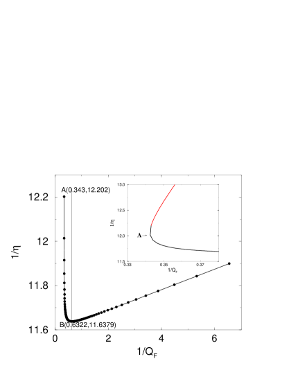
FIG. 7.: The relation between efficiency and cooling power for the heat pump. The parameters are: The constant optimal cycle time, $\tau$, =0.78; T_c=51.49, T_h=257.45, $\omega_{a}$=47.699, $\omega_{b}$=600, $\Gamma_{c}$=1, $\Gamma_{h}$=2, $\sigma$=0.005 Left: Comparison between $1/{\cal Q}_{F}$(plot 1) and $1/\eta$(plot 2) as a function of the allocated time transfer from the heat exchange branches to the ’adiabats’. Zero time is the optimal heat-flow time allocation. Right: The Universal plot for the heat pump. The starting optimal point in the plane of ($1/{\cal Q}_{F}$, $1/\eta$), was (0.34296, 12.202), while the maximum efficiency point $\bf B$ is (0.6322,11.6379) and time allocation $(\tau_{c},\tau_{h},\tau_{a},\tau_{b})$= (0.22721,0.16328,0.1636,0.2259). The insert shows the neighborhood of point $\bf A$.

Point $\bf A$ is located at the maximum cooling power. If more time is allocated to the heat exchange branches both $1/{\cal Q}_{F}$ and $1/\eta$ will continue to increase as seen in the insert of Fig. 7.

(c) Optimization with respect to the fields.

The values of the fields $\omega_{a}$ and $\omega_{b}$ are control parameters of the engine. In a spin system these fields are equivalent to the value of the external magnetic field applied on the system. They directly influence the energy spacing of the TLS. The work function ${\cal W}_{cycle}$, or equivalently the power ($\cal P$) is optimized with respect to the fields, subject to the Carnot constraint:

$${\omega_{a}\over T_{c}}~{}\geq~{}{\omega_{b}\over T_{h}}$$ (67)

Optimal power is obtained by equating independently to zero the partial derivatives of $~{}~{}{\cal W}_{cycle}$, or of ${\cal P}~{}=~{}~{}{\cal W}_{cycle}/\tau$ by varying $\omega_{a}$ and $\omega_{b}$. In addition the optimal solutions have to fulfill the inequality constraints in Eq. (67). As a result two transcendental equations in $\omega_{a}$ and $\omega_{b}$ are obtained which are solved numerically.

The two equations are:

$$\begin{array}[]{r}~{}{(1~{}-~{}y~{}x_{max})\over(\omega_{b}~{}-~{}\omega_{a})}~{}({\Delta S^{eq}~{}+~{}\sigma^{2}/\tau_{a}})~{}\cosh^{2}\left({{\omega_{a}}\over{2k_{B}T_{c}}}\right)~{}=~{}{~{}1-y\over(4~{}k_{B}~{}T_{c})}\\ ~{}{(x_{max}~{}-~{}x)\over(\omega_{b}~{}-~{}\omega_{a})}~{}({\Delta S^{eq}~{}+~{}\sigma^{2}/\tau_{a}})~{}\cosh^{2}\left({{\omega_{b}}\over{2k_{B}T_{h}}}\right)~{}=~{}{~{}1-x\over(4~{}k_{B}~{}T_{h})}\end{array}$$ (70)

Where $\Delta S^{eq}$= S${}_{h}^{eq}$- S${}_{c}^{eq}$ as defined in Eq. (36). Examining Eq. (70), and fixing the friction $\sigma$, it is found that $\Delta S^{eq}$ is an extensive function of order zero (intensive ) with respect to the quartet of variables $\omega_{a},T_{c},\omega_{b},T_{h}$. This means that scaling these parameters simultaneously will not change $\Delta S^{eq}$. Also x_max, and $\cosh^{2}\left({{\omega}\over{2k_{B}T}}\right)$ are extensive (order zero). The work function however, is extensive with order one (Eqs. (51) and (52)). This property will be exploited in paragraph III.

The optimization of power with respect to the fields is shown in Fig. 8 for the frictionless engine, as a function of the fields with fixed time allocation. A global maximum can be identified.

FIG. 8.: Power for the frictionless engine as a function of the fields ($\omega_{a}$, $\omega_{b}$) for constant bath temperatures, and constant time allocations. The maximum power is achieved at $\omega_{a}=1794$ and $\omega_{b}=4239$ where the bath temperatures are $T_{c}=500,T_{h}=2500$.

The heat pump optimization of ${\cal Q}_{F}$ with respect to the fields is different and therefore will be presented in Section III.

The analysis for the optimization with respect to the fields for the entropy production $\Delta{\cal S}^{u}$, is presented in appendix C. The optimal solution without friction($\sigma=0$) leads to $\Delta{\cal S}^{u}_{min}=0$. When $\sigma\neq 0$, the minimum value of $\Delta{\cal S}^{u}$ is different from zero, and is achieved on the boundary of the region.

E Global Optimization of the Heat Engine

Global optimization of the power means searching for the optimimum with respect to the control parameters cycle time, time allocation and the fields. An iterative procedure is used.

The procedure is initiated by setting the optimal time allocation from the corresponding Lagrangian, with $\sigma=0$. The power becomes a product of two functions, one depending only on time the other only on the fields, and therefore, the fields can be changed independently of time. The optimal fields for the above time allocation are then sought. For the frictionless case, the overall time on the adiabats tends to zero. The optimal field values become independent of time. The value ${\cal P}=107.501$ is the short time limit in accordance with the equation:

$${\cal P}~{}~{}\longrightarrow~{}~{}(\omega_{b}-\omega_{a})(S_{h}^{eq}-S_{c}^{eq})(\Gamma_{c}\Gamma_{h})/(\sqrt{\Gamma_{c}}+\sqrt{\Gamma_{h}})^{2}$$ (71)

These fields are inserted into the expression with friction $\sigma\neq 0$, and the new optimal times and fields are computed. The iteration converges after two to three steps, as indicated by Table IV for $\sigma=0.005$. Notice that the location of the optimum is not very sensitive to the friction parameter.

TABLE III.: Global optimization of power. The notation ${\cal P}^{max}(\omega_{a},\omega_{b})$ stands for fixed time allocations, and the notation ${\cal P}^{max}(\tau_{a},\tau_{b})$ stands for fixed field values. The other parameters are: $T_{c}=500$, $T_{h}=2500$, $\tau_{a}$= $\tau_{b}$=0.01. $\Gamma_{c}=1$ and $\Gamma_{h}=2$

$\sigma$	$\tau$	${\cal P}^{max}(\omega_{a},\omega_{b})$	${\cal P}^{max}(\tau_{c},\tau_{h})$	$\omega_{a}$	$\omega_{b}$	$\tau_{c}/\tau$
0.005	2		84.46	1794	4239	0.5999
0.005	1.367		87.18	1794	4239	0.5891
0.005	1.367	88.68		1719.1	4036.31	0.5891
0.005	1.347		87.47	1719.1	4036.31	0.58856
0.005	1.347	88.704		1718.16	4033.67	0.58856

In Table IV, the extensive properties Eq. (70) are examined for k=2 and k=10 with respect to Table IV. The temperature values will change to T${}_{c}~{}=~{}1000$, T${}_{h}~{}=~{}5000$ for k=2 and T${}_{c}~{}=~{}5000$, T${}_{h}~{}=~{}25000$ for k=10 . The results verify the analysis.

TABLE IV.: Global optimization of power. By multiplying the four values, T_c, T_h, $\omega_{a}$, $\omega_{b}$ by k and searching first for optimal time allocation, then multiplying only the temperature values by k and searching for the optimal fields. All the notations and other parameters as in Table IV.

$\sigma$	k	$\tau$	${\cal P}^{max}(\omega_{a},\omega_{b})$	${\cal P}^{max}(\tau_{c},\tau_{h})$	$\omega_{a}$	$\omega_{b}$	$\tau_{c}/\tau$
0.005	2	1.367		174.9	3438.2	8072.6	0.58852
0.005	2	1.367	174.9		3436.7	8070.3	0.58852
0.005	2	1.347		174.94	3436.7	8070.3	0.58856
0.005	2	1.347	179.8		3437.7	8069.4	0.58856
0.005	10	1.347	887.04		17181.6	40336.7	0.58856

III Asymptotic Properties of the Heat Pump when the cold bath temperature approaches absolute zero.

The goal is to obtain an asymptotic upper bound on the cooling power when the heat pump is operating close to absolute zero temperature. This requires optimizing the performance of the heat pump with respect to all control parameters.

A Optimization of the heat-flow ${\cal Q}_{F}$ with respect to the fields and to the cooling power upper bound.

The heat-flow,${\cal Q}_{F}$ extracted from the cold reservoir now becomes the subject of interest:

$$~{}~{}~{}{\cal Q}_{F}~{}~{}~{}=\omega_{a}(S_{2}-S_{1})/\tau$$ (72)

or from Eq. (43),

$$~{}~{}~{}{\cal Q}_{F}~{}~{}~{}=(\omega_{a}/\tau)\left((S_{2}^{eq}-S_{1}^{eq})F(x,y)~{}-~{}{\sigma^{2}(1-x)(y/\tau_{a}+1/\tau_{b})\over(1-xy)}\right)$$ (73)

No global maximum for the ${\cal Q}_{F}$ with respect to the fields is found. The derivative of ${\cal Q}_{F}$ with respect to $\omega_{b}$ becomes:

$${{\partial{{\cal Q}_{F}}}\over{{\partial{\omega_{b}}}}~{}}=~{}~{}{~{}F(x,y)~{}\omega_{a}\over\tau~{}}~{}{1\over 4~{}k_{B}~{}T_{h}~{}\cosh^{2}{\omega_{b}\over 2~{}k_{B}~{}T_{h}}}\geq 0$$ (74)

leading to the result that ${\cal Q}_{F}$ is monotonic in $\omega_{b}$. Under such conditions, $\omega_{b}$ is set, and the optimum with respect to $\omega_{a}$ is sought for. The derivative of ${\cal Q}_{F}$ with respect to $\omega_{a}$ becomes:

$${{\partial{{\cal Q}_{F}}}\over{{\partial{\omega_{a}}}}}~{}=(S_{2}^{eq}-S_{1}^{eq})~{}-~{}{\sigma^{2}\over(1-y)}(y/\tau_{a}+1/\tau_{b})~{}-~{}\omega_{a}~{}{1\over 4~{}k_{B}~{}T_{c}~{}\cosh^{2}{\omega_{a}\over 2~{}k_{B}~{}T_{c}}}~{}=~{}0$$ (75)

Introducing from Eq. (75) the optimal value of $(S_{2}^{eq}-S_{1}^{eq})~{}-~{}{\sigma^{2}\over(1-y)}(y/\tau_{a}+1/\tau_{b})$, into Eq. (73), leads to the optimal cooling rate:

$$~{}~{}~{}{\cal Q}_{F}^{optimum}~{}~{}~{}=~{}~{}{~{}F(x,y)~{}\omega_{a}^{2}\over\tau~{}}~{}{1\over 4~{}k_{B}~{}T_{c}~{}\cosh^{2}{\omega_{a}\over 2~{}k_{B}~{}T_{c}}}~{}=~{}~{}{~{}F(x,y)~{}\over 4~{}k_{B}~{}\tau~{}}~{}\left({~{}\omega_{a}\over~{}T_{c}~{}}\right)^{2}~{}{T_{c}\over\cosh^{2}{\omega_{a}\over 2~{}k_{B}~{}T_{c}}}$$ (76)

Due to its extensivity, the ratio ${\omega_{a}\over T_{c}}$ becomes a constant, while both $\omega_{a}$ and T_c can approach zero.

From Eq.(76), an upper-bound for the cooling rate ${\cal Q}_{F}$ is obtained:

$$~{}~{}~{}{\cal Q}_{F}^{optimum}~{}~{}~{}\leq~{}~{}~{}{~{}F(x,y)~{}\over 4~{}k_{B}~{}\tau~{}}~{}\left({~{}\omega_{a}\over~{}T_{c}~{}}\right)^{2}~{}T_{c}.$$ (77)

From Eqs. (77), when T_c approaches zero, the cooling rate vanishes, at least linearly with temperature. This is a third law statement which shows that absolute zero cannot be reached since the rate of cooling vanishes as absolute zero is approached.

B The asymptotic relation between the internal and external temperature on the cold branch

When the bath temperature tends to zero, the internal working fluid temperature has to follow. This becomes a linear relationship between $T^{\prime}$ and $T_{c}$ as $T_{c}$ tends to zero.

Calculating the polarization at the end of the contact with the cold bath $S_{2}$:

$$S_{2}=S_{2}^{eq}~{}-~{}{(S_{2}^{eq}-S_{1}^{eq})x(1-y)~{}-~{}\sigma^{2}x(1/\tau_{b}~{}+y/\tau_{a})\over(1-xy)}$$ (78)

Assuming the relation $T_{h}$ = $\rho$ $T_{c}$ as $T_{c}$ tends to zero, the exponents can be expanded to the first order to give:

$${S_{2}}=~{}{T_{c}\over\omega_{a}}{1-xy_{max}+(\omega_{a}/\omega_{b})\rho x(y_{max}-y)\over(1-xy)}~{}~{}+~{}~{}1/2~{}-~{}{x(\sigma^{2}/\tau_{a})(y_{max}-y)\over(1-xy)}$$ (79)

Also, $S_{2}$ defines the internal temperature $T^{\prime}$ through the relation: ${S_{2}}~{}=~{}-{1\over 2}\tanh\left({{\omega}_{a}\over{2k_{B}T^{\prime}}}\right)~{}~{}$. Expanding the hyperbolic tangent, one gets:

$${T^{\prime}}~{}~{}=~{}~{}{T_{c}}~{}{1~{}-~{}xy_{max}~{}+~{}\rho(\omega_{a}/\omega_{b})x(y_{max}-y)\over(1-xy)}~{}~{}-~{}~{}{x\omega_{a}(\sigma^{2}/\tau_{a})(y_{max}-y)\over(1-xy)}$$ (80)

proving that $T_{c}$ and $T^{\prime}$ both tend asymptotically to zero. It should be noted that the term independent of $T_{c}$ depends on $\omega_{a}$, which also tends to zero as $T_{c}$ tends to zero ( (Eq. 77). Eq. (77) also shows that ${\cal Q}_{F}^{optimum}$*T_c is a quadratic function of $\omega_{a}$, Cf. Fig. 9.

Eq. (77) represents an upper-bound to the rate of cooling. In order to determine how closely this limit be approached, a strategy of cooling must be devised, which re-optimizes the cooling power during the changing conditions when T_c approaches zero.

C Optimal cooling strategy

The goal is to follow an optimal cooling strategy, which exploits the properties of the equations and achieves the upper-bound for the rate of cooling, ${\cal Q}_{F}$.

The properties of the equations employed are;

• i: The derivative with respect to $\omega_{a}$ of ${\cal Q}_{F}$ ( Eq. (75)), is extensive of order zero in the ’quartet’ ($\omega_{a},\omega_{b},T_{c},T_{h}$).

• ii: For ${\partial{{\cal Q}_{F}}}\over{{\partial{\omega_{a}}}}$ the extensivity holds also for the ’doublets’ ($\omega_{b}~{},~{}T_{h}$) or ($\omega_{a}~{},~{}T_{c}$). Scaling these variables by the same number, leaves Eq. (75) equal to zero, and the value of ${\cal Q}_{F}^{optimum}$ does not change.

• iii: In spite of ${\cal Q}_{F}$ being monotonic in $\omega_{b}$, $~{}{\cal Q}_{F}^{optimum}$ is independent of $\omega_{b}$ (and of T_h), therefore ${\cal Q}_{F}$ saturates as $\omega_{b}$ is increased.

From property (i) it follows, that once an optimal ’quartet’($\omega_{a},\omega_{b},T_{c},T_{h}$) is created, it is possible to cool optimally with a set of quartets, which are scaled by a decreasing set $r_{n}~{}<~{}1$, $\lim_{n\rightarrow\infty}r_{n}=0$. For this set the limit of the ratio ${\omega_{a}\over T_{c}}$ is a non zero constant. Therefore in Eq. (76) $\omega_{a}$ and T_C are optimal leading to:

$$~{}~{}~{}{\cal Q}_{F}^{optimum}~{}~{}~{}=~{}{~{}F(x,y)~{}\over 4~{}k_{B}~{}\tau_{optimal}~{}}~{}\left({~{}\omega_{a,optimal}\over~{}T_{c,optimal}}\right)^{2}~{}{T_{c,optimal}\over\cosh^{2}{\omega_{a,optimal}\over 2~{}k_{B}~{}T_{c,optimal}}}$$ (81)

In general, the hot bath temperature is constant, and the property (ii) is used to scale back the value of the optimal T_h to the bath temperature. As a result, the optimal high field is also scaled.

Property (iii) will be exploited by changing only $\omega_{b}$ in the optimal quartets and checking for saturation. See Fig. 13 and the dashed curves of Fig. 9. Summarizing, for every ’quartet’ the upper-bound in Eq. (77) can be reached. The details of the cooling strategy can be found in Appendix E

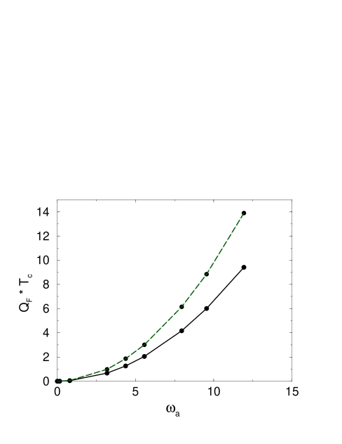
FIG. 9.: Left, (solid line): The optimal heat-flow ${\cal Q}_{F}^{optimum}$ for the heat pump as a function of T_c. The fixed parameter values of the pair ($\omega_{b}$ and T_h) are, T${}_{h}=64.359,51.49,42.9082,30.03555,23.599,17.153,4.291,0.8582,0.1717,0.01717$, and accordingly $\omega_{b}=150,120,100,70,55,40,10,2,0.4,0.04$. The other constant parameter values are: $\sigma=0.005$, $\Gamma_{c}=1$, $\Gamma_{h}=2$. (dashed line): fixing $\omega_{b}~{}=~{}3000$ for every point. The other parameters are the same as the solid line. Right: The optimal heat-flows multiplied by the corresponding T_c as a function of $\omega_{a}$. The optimal time is constant for the chosen parameters; $\tau_{optimal}=0.885$ for the solid curves, and 0.825 for the dashed curves.

Fig. 10 shows that the cooling strategy ( Tables V and VI ) can approach the upper bound leading to a linear relation of the optimal cooling power with temperature. With respect to the fields the optimal strategy leads to a decrease of the field $\omega_{a}$ which is in contact with the cold bath. This causes the internal temperature of the TLS T’ to be lower than the cold bath temperature T_c. On the hot side the optimal solution requires as large an energy separation as possible $\omega_{a}\rightarrow\infty$ but this effect saturates.

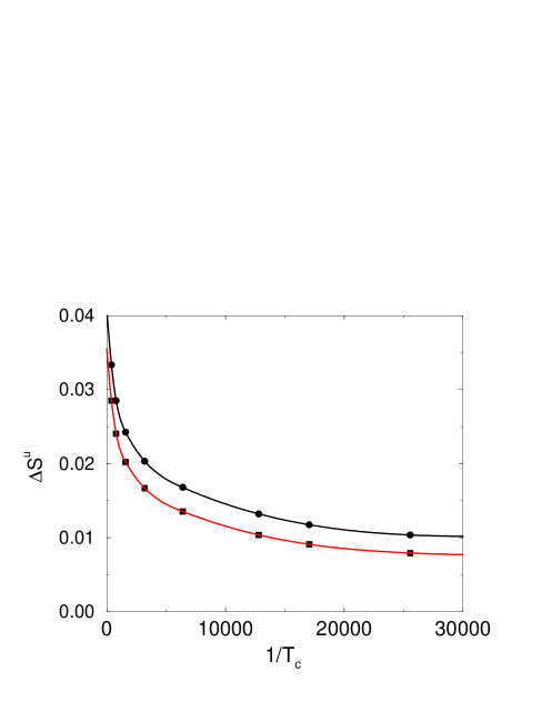
FIG. 10.: Left: The optimal cooling rate as a function of the cold bath temperature T_c, compared with the upper-bound for the cooling rate. Right: The entropy production during cooling shown for the case with friction (upper line, circles) and without friction (lower line, squares). The common parameters for all three figures are: $\tau_{a}=\tau_{b}=0.01$, $\sigma=0.005$, $\Gamma_{c}=1$, $\Gamma_{h}=2$.

The linear relation of the cooling rate with T_c leads to a constant asymptotic entropy production as can be seen in the right of Fig. 10 ( Cf. Appendix C).

IV Conclusion

The detailed study of the four stroke discrete heat engine with internal friction serves as a source of insight on the performance of refrigerators at temperatures which are very close to absolute zero. The next step is to find out if the behavior of the specific heat pump described in the study can be generalized. A comparison with other systems studied indicates that the conclusions drawn from the model are generic. As a heat engine the model shows the generic behavior of maximum power as a function of control parameters found in finite time thermodynamics [3, 4, 5, 6]. This is despite the fact that the heat transfer laws in the microscopic model of the working fluid are different from the macroscopic laws such as the Newtonian heat transfer law [16]. When operated as a heat pump with friction, the present model shows the universal behavior observed for commercial chillers [27] caused by a tradeoff between allocating resources to the ’adiabats’ or to the heat exchange branches.

Another question is whether the linear scaling of the optimal cooling power at low cold bath temperatures is a universal phenomenon. For low temperatures the results of the present model can be extended to a working fluid consisting of an ensemble of harmonic oscillators or any N-level systems. This is because at the limit of absolute zero only the two lowest energy levels are relevant. When examined, other models with different operating cycles show an identical behavior. For example the continuous model of a quantum heat engine [18] based on reversing the operation of a laser shows this linear scaling phenomena. Another example is the Ericsson refrigeration cycle Cf. Eq. (23) in the study of Chen et al [25] which shows the same asymptotic linear relationship.

A point of concern is the dependence of the heat transfer laws on temperature when absolute zero is approached. The kinetic parameters $k_{\downarrow}$ and $k_{\uparrow}$ represent an individual coupling of the two-level-system to the bath. Considering coefficients derived from gas phase collisions they settle to a constant asymptotic value as the temperature is lowered [29]. The reason is that the slow approach velocity is compensated by the increase in the thermal De-Broglie wavelength.

There has been an ongoing interest in the meaning of the third law of thermodynamics [30, 31, 32, 33, 34, 35, 36]. The issue at stake has been: is the third law an independent postulate or it is a consequence of the second law and the vanishing of the heat capacity. This study presents a dynamical interpretation of the third law. The absolute temperature cannot be reached because the maximum rate of cooling vanishes linearly at least with temperature.

A Analysis for the ’moving’ Cycles.

Insight into the origin of the behavior of the ’moving’ cycles is seen in Fig. 11, where the polarizations S₁, S₂ are shown as monotonically decreasing functions of the time allocation on the cold bath. However, the envelope of S₁ for maximal power, namely for maximal S₁-S₂ is worth noticing. It is a decreasing function for short cycle times, achieves a minimum at $\tau_{0}$, and starts to increase for $\tau~{}>~{}\tau_{0}$. Thus it is responsible for shifting the cycles to smaller polarization for short cycle times, and for the change of that trend for larger cycle times. The envelope of S₂ for maximal S₁-S₂ is also a monotonically decreasing function of $\tau_{c}$, or equivalently of $\tau$, supporting the increase of S₁-S₂. The figure also shows, that for a short time allocation both S₁ and S₂ are close to the equilibrium polarization S${}_{h}^{eq}$, When not enough time is allocated on the hot bath both the polarizations S₁ and S₂ approach S${}_{c}^{eq}$.

FIG. 11.: Comparison between the polarizations S₁ and S₂ as a function of $\tau_{c}$, for ten different $\tau$ values, 0.06, 0.08, 0.1, 0.25, 0.5, 0.75, 1 1.25, 1.5 and 2. The solid curves are S₁ while the dashed curves are S₂. Superimposed are the values of S₁ and S₂ for the maximal S₁ -  S₂.

B The computation of $\tau_{0}$

The computation of $\tau_{0}$ Eq. (48) is not sufficient since it gives only the relation between the times spent on the cold and hot branches for zero work. The natural additional requirement is to seek for the optimal allocations, $\tau_{c,0}$ and $\tau_{h,0}$ using Eq. (63): $\tau_{0}$ = $\tau_{c,0}$ + $\tau_{h,0}$ + $\tau_{a}$ + $\tau_{b}$

Denoting by $x_{0}$ and $y_{0}$ the corresponding x and y values defined in Eq. (21), the following two equations for x₀ and y₀ are obtained:

$$y_{0}~{}=~{}{(x_{max}~{}-~{}x_{0})~{}-~{}{R}\over(x_{max}~{}-x_{0})~{}-~{}{Rx_{0}}}$$ (B1)

and

$$\Gamma_{c}~{}x_{0}\left((1-y_{0})(1~{}-~{}y_{0}~{}x_{max})\right)~{}=~{}\Gamma_{h}~{}y_{0}\left((1-x_{0})(x_{max}~{}-~{}x_{0})\right)$$ (B2)

Where R is defined as:

$$R~{}=~{}{\sigma^{2}~{}\omega_{a}~{}(1/\tau_{a}~{}+~{}1/\tau_{b})~{}\over(\omega_{b}~{}-~{}\omega_{a})~{}(S_{h}^{eq}~{}-S_{c}^{eq}~{}+~{}\sigma^{2}/{\tau_{a}})}$$ (B3)

and x_max was defined in Eq. (38) as:

$$x_{max}~{}=~{}{(S_{h}^{eq}~{}-~{}S_{c}^{eq})~{}-~{}{\sigma^{2}/\tau_{b}}\over(S_{h}^{eq}~{}-S_{c}^{eq})~{}+~{}{\sigma^{2}/\tau_{a}}}$$ (B4)

The quadratic equation to be solved for x₀ is,

$$AA~{}x_{0}^{2}~{}+~{}BB~{}x_{0}~{}+~{}CC~{}=~{}~{}0$$ (B5)

Where AA = $\Gamma_{h}$ (1 + R)   BB = - ($\Gamma_{h}$ ((1 + R) (x_max-R) + x_max)  + $\Gamma_{c}$ (1 + R - $x_{max}$)) and CC = $\Gamma_{h}$ (x_max-R) x_max

C Entropy production.

(1) Heat Engine.

$$\Delta{\cal S}^{u}_{cyle1}~{}=~{}-({\cal Q}_{AB}/T_{h}~{}+~{}{\cal Q}_{CD}/T_{c})$$ (C1)

Or from Table (I)

$$\Delta{\cal S}^{u}_{cyle1}~{}=~{}(\omega_{a}/T_{c}-\omega_{b}/T_{h})(S_{1}-S_{2})~{}+~{}{\sigma^{2}\omega_{a}\over{T_{c}}}(1/\tau_{a}~{}+~{}1/\tau_{b})$$ (C2)

The entropy production results are shown in Fig. 12. The left figure shows $\Delta{\cal S}^{u}$ with increasing friction. The middle figure shows the corresponding cycles, while the right figure shows the corresponding power values.

FIG. 12.: Left: The entropy production of the heat engine as a function of the time spent on the cold branch for the fixed values of $\omega_{a}=1794$, $\omega_{b}=4238$, $T_{c}=500$, $T_{h}=2500$, $\Gamma_{c}=1$, $\Gamma_{h}=2$  and $\tau=0.1$. Middle: The corresponding cycles. Right: The corresponding powers. Seven cases are shown. Case ’00’ is the frictionless case, when the times spent on the ’adiabats’, are zero, case ’01’ is the frictionless case, when the times spent on the ’adiabats’, $\tau_{a}$ and $\tau_{b}$ are different from zero and equal: 0.01. The other five cases are with increasing friction, when also $\tau_{a}=\tau_{b}~{}=~{}0.01$, whereas the different friction coefficients $\sigma$ are: for plot  1: $\sigma=0.003$, for plot  2: $\sigma=0.004$,  for plot  3: $\sigma=0.005$, for plot 4: $\sigma=0.006$ and for plot  5: $\sigma=0.007$.

The reciprocal behavior of the entropy production and the power is clear from Fig. 12. One also observes, that for the given cycle time the ’free’ time for the cycles with increasing $\sigma$ becomes more restricted. This follows from the dependence of $\tau_{c,min}$ on $\sigma$. See also Fig.( 3)

Introducing Eq. (36) into Eq. (C2). The entropy production becomes,

$$\Delta{\cal S}^{u}_{cyle1}~{}=~{}(\omega_{a}/T_{c}-\omega_{b}/T_{h})(S_{h}^{eq}-S_{c}^{eq})F(x,y)~{}+~{}\Delta{\cal S}^{u}_{\sigma 1}$$ (C3)

where

$$\Delta{\cal S}^{u}_{\sigma 1}~{}=~{}\sigma^{2}{1\over(1-xy)}\left({{\omega_{a}\over T_{c}}}{(1-x)}(1/\tau_{a}~{}+~{}y/\tau_{b})~{}+~{}{{\omega_{b}\over T_{h}}}{(1-y)}(x/\tau_{a}~{}+~{}1/\tau_{b})\right)$$ (C4)

Notice, that $\Delta{\cal S}^{u}_{\sigma 1}$ is always positive. For $\sigma=0$ Eq. (C4) reduces to the frictionless results [20].

(2) Heat Pump

The entropy production for the heat pump becomes:

$${\Delta{\cal S}^{u}}_{ref}=\left({\omega_{b}\over T_{h}}-{\omega_{a}\over T_{c}}\right)(S_{2}-S_{1})~{}+~{}\sigma^{2}{\omega_{b}~{}\over T_{h}}(1/\tau_{a}~{}+~{}1/\tau_{b})$$ (C5)

$$~{}~{}=~{}~{}\left({\omega_{b}\over T_{h}}-{\omega_{a}\over T_{c}}\right)(S_{2}^{eq}-S_{1}^{eq})\cdot F(x,y)~{}+~{}$$ (C6)

$$\sigma^{2}F(x,y)\left\{\frac{\omega_{b}}{T_{h}}\frac{1}{1-x}(\frac{1}{\tau_{a}}~{}+~{}\frac{x}{\tau_{b}})~{}+~{}\frac{\omega_{a}}{T_{c}}\frac{1}{1-y}(\frac{1}{\tau_{b}}~{}+~{}\frac{y}{\tau_{a}})\right\}$$ (C7)

The asymptotic entropy production as T_c tends to zero can be calculated leading to

$${\Delta{\cal S}^{u}_{ref}}~{}=~{}F(x,y)~{}[(\omega_{b}/(\rho\omega_{a}))(1-\rho(\omega_{a}/\omega_{b}))^{2}~{}+~{}$$ (C8)

$$\sigma^{2}~{}\left({\omega_{b}\over\rho T_{c}}{1\over(1-x)}(1/\tau_{a}+x/\tau_{b})~{}+~{}{\omega_{a}~{}\over T_{c}}{1\over(1-y)}(1/\tau_{b}+y/\tau_{a})\right)]$$ (C9)

Since $T_{h}=~{}\rho T_{c}$, the r.h.s. of Eq. (C9) tends to a constant, for each term depends on the constant ratios ($\omega_{b}$/T_h), ($\omega_{a}$/T_c) or on their ratio. This result is demonstrated on the right side of Fig. 10.

The optimization with respect to time allocation has the same result as for the heat engine. Therefore, only optimization with respect to the fields are presented;

Equating to zero the derivatives with respect to x an y of the entropy production, one gets two similar equation to the total work derivatives:

$$~{}{(1~{}-~{}y~{}x_{max})\over({\omega_{a}}/{T_{c}}~{}-~{}{\omega_{b}}{T_{h}})}~{}({\Delta S^{eq}~{}+~{}\sigma^{2}/\tau_{a}})~{}\cosh^{2}\left({{\omega_{a}}\over{2k_{B}T_{c}}}\right)~{}+~{}{~{}1-y\over(4~{}k_{B}~{}T_{c})}~{}\geq 0$$ (C10)

$$~{}{(x_{max}~{}-~{}x)\over({\omega_{a}}/{T_{c}}~{}-~{}{\omega_{b}}{T_{h}})}~{}({\Delta S^{eq}~{}+~{}\sigma^{2}/\tau_{a}})~{}\cosh^{2}\left({{\omega_{b}}\over{2k_{B}T_{h}}}\right)~{}+~{}{~{}1-x\over(4~{}k_{B}~{}T_{h})}~{}\geq 0$$ (C11)

Where $\Delta S^{eq}$, is $S_{h}^{eq}$- $S_{c}^{eq}$.

Eqs. (C10) and (C11) show that the entropy production is a monotonic function in the allowed range, namely, for

$${\omega_{a}\over T_{c}}>{\omega_{b}\over T_{h}}.$$ (C12)

To conclude the entropy production has a minimum value: $\Delta{\cal S}^{u}_{min}$, will be

$${\Delta{\cal S}^{u}_{min}}~{}=~{}{\omega_{a}\over T_{c}}\sigma^{2}(1/\tau_{a}+1/\tau_{b})$$ (C13)

obtained on the boundary of the range.

D The Total Work done on the System for the Heat Pump

The total work done on the system becomes,

$${\cal W}_{cyle3}^{on}=(\omega_{b}-\omega_{a})(S_{2}-S_{1})~{}+~{}\sigma^{2}\omega_{b}~{}(1/\tau_{a}~{}+~{}1/\tau_{b})$$ (D1)

or

$${\cal W}_{cyle3}^{on}=(\omega_{b}-\omega_{a})(S_{2}^{eq}-S_{1}^{eq})F(x,y)~{}+~{}W_{\sigma 3}$$ (D2)

where

$${\cal W}_{\sigma 3}~{}=~{}{\sigma^{2}\over(1-xy)}\left(\omega_{b}(1-y)({1/\tau_{a}}~{}+~{}{x/\tau_{b}})~{}~{}+~{}~{}\omega_{a}(1-x)({y/\tau_{a}}~{}+~{}{1/\tau_{b}})\right)~{}~{}$$ (D3)

$$~{}~{}=~{}~{}\sigma^{2}F(x,y)\left\{\frac{\omega_{b}}{1-x}(\frac{1}{\tau_{a}}~{}+~{}\frac{x}{\tau_{b}})~{}+~{}\frac{\omega_{a}}{1-y}(\frac{1}{\tau_{b}}~{}+~{}\frac{y}{\tau_{a}})\right\}$$ (D4)

Eq. (D1) can be interpreted as the work done on the working fluid see (Cf. Fig. 2), as the sum of three positive areas, $(\omega_{b}~{}-~{}\omega_{a})(S_{2}~{}-~{}S_{1})$, $\sigma^{2}\omega_{b}(1/\tau_{a})$ and  $\sigma^{2}\omega_{b}(1/\tau_{b})$ with the corresponding corners, D,C,B¹,A¹,  B,B¹,S₂,S₃ and A¹,A,S₄,S₁.

E The optimal cooling strategy close to the absolute zero temperature

The first step in the cooling strategy is to create the first optimal quartet;

• (0) The systems external parameters $\sigma$, $\tau_{a}$, $\tau_{b}$, $\Gamma_{c}$ and $\Gamma_{h}$ are set.

• (1) A decreasing set of $\omega_{b}$ is chosen.

• (2) A constant ratio ($\rho$) for T_h/T_c, is chosen which is the ratio of the initial bath temperatures.

• (3) For the above chosen values, the optimal values of $\omega_{a}$, T_c, $\tau$, and its optimal allocations between the branches to give maximal Q_F are found for each $\omega_{b}$ in the set in (1) , by solving numerically the following additional equation to Eq. (75), with the condition that T${}_{h}~{}=~{}\rho\cdot$T_c:

  $$~{}{{\partial{{\cal Q}_{F}}}\over{{\partial{T_{c}}}}}~{}=~{}{F(x,y)~{}\over\ {4~{}\tau~{}~{}k_{B}}~{}}~{}\left(~{}{\omega_{a}\over T_{c}}\right)^{2}~{}\left({1\over\cosh^{2}{\omega_{a}\over 2~{}k_{B}~{}T_{c}}}~{}-~{}{\omega_{b}\over\rho\omega_{a}~{}\cosh^{2}{\omega_{b}\over 2\rho~{}k_{B}~{}T_{c}}}\right)~{}=~{}0$$ (E1)

The above strategy causes the decrease of $T_{h}$ together with the $T_{c}$. Nevertheless according to (ii) above, the doublet $\omega_{b}$ and $T_{h}$ can be rescaled to increase $T_{h}$ back to its original value. The solid curves of Fig. 9 are optimal in the in the above described sense. Increasing only the value of $\omega_{b}$ in the optimal quartet according to point (iii), leads to larger values of the cooling rate, but eventually the increase of ${\cal Q}_{F}$ will slow down and saturate. See Fig. 13 and the dashed curves of Fig. 9.

Fig. 13 represents the saturation phenomenon on $\omega_{b}$. Three points from Fig. 9 are chosen, and all parameters are fixed, except $\omega_{b}$, which is allowed to increase.

FIG. 13.: Left: The optimal heat-flow for the heat pump as a function of $\omega_{b}$, showing the saturation phenomenon. The fixed parameter values are: for triangles; $T_{h}=64.5725$, $T_{c}=12.9145$, $\omega_{a}=11.9233$,  starting with $\omega_{b}~{}=~{}150$, for squares; $T_{h}=42.90815$, $T_{c}=8.58168$, $\omega_{a}=7.94986$,  starting with $\omega_{b}~{}=~{}100$, for circles; $T_{h}=23.59905$, $T_{c}=4.71981$, $\omega_{a}=4.37247$,  starting with $\omega_{b}~{}=~{}55$. The common parameters for all three figures are: $\tau_{a}=\tau_{b}=0.01$, $\sigma=0.005$, $\Gamma_{c}=1$, $\Gamma_{h}=2$. Right: The optimal heat-flows as a function of $\tau_{max}$, the time at which the optimum is achieved. The fixed parameter values are the same, as on the left. We note, that the optimal time is becoming constant only at saturation.

In order to approach the upper-bound for ${\cal Q}_{F}$ in Eq. (77), a decreasing set of $\omega_{a}~{}/~{}T_{c}$ is created, achieved in an optimal way:

First step: After having an optimal ’quartet’, T_c and T_h, are fixed. Then, by lowering $\omega_{b}$, one finds the corresponding optimal $\omega_{a}$ values. This procedure is checked globally, by also iterating the time allocations. The results of a typical example are shown in Table V.

Second step: Using again the property of extensivity, the cooling will be achieved by multiplying the rows of Table V by a decreasing sequence, e.g. by $2^{-n}$ for the n-th row. Table VI describes the cooling strategy, checking also the non-divergence of the entropy production both for the frictionless case and the case with friction. The results are also summarized in Fig. 10.

Table V demonstrates, that the procedure shifts down to the Carnot bound. The ratio R =  ${\omega_{b}\over T_{h}}$/ ${\omega_{a}\over T_{c}}$. was computed showing only small changes.

TABLE V.: First step. Starting from an optimal quartet, the procedure creates for a given decreasing set of $\omega_{b}$-s, a decreasing set of of $\omega_{a}$-s for fixed bath temperatures.

$T_{c}$	Th	$\omega_{b}$	$\omega_{a}^{optimal}$	$\omega_{a}^{optimal}/T_{c}$	$\omega_{b}/T_{h}$	R	${\cal Q}_{F}$
0.0025	50	60	1.370(-3)	0.5392	1.2	2.226	5.812(-5)
0.0025	50	55	1.273(-3)	0.5090	1.1	2.161	5.013(-5)
0.0025	50	50	1.164(-3)	0.4653	1	2.149	4.241(-5)
0.0025	50	45	1.051(-3)	0.4205	0.9	2.140	3.50549(-5)
0.0025	50	40	9.320(-4)	0.3728	0.8	2.146	2.826(-5)
0.0025	50	35	8.250(-4)	0.3300	0.7	2.121	2.182(-5)
0.0025	50	30	6.985(-4)	0.2794	0.6	2.147	1.613(-5)

TABLE VI.: A procedure to get an optimal set of pairs of $\omega_{a},~{}T_{c}$ where their ratio tends to zero. T${}_{h}=~{}50$ for every cold bath temperature, T_c. The index ’fl’ stands for the frictionless case, and $Q_{F}^{up}$ denotes the upper-bound for ${\cal Q}_{F}$.

$T_{c}$	$\omega_{b}$	$\omega_{a}^{optimal}$	$\Delta S^{u}$	$\Delta S^{u,fl}$	${\cal Q}_{F}$	${\cal Q}_{F}^{up}$
0.0025	60	1.370(-3)	0.0333353	0.0285	5.812(-5)	6.084(-5)
0.00125	55	6.365(-4)	0.0285075	0.02406	2.457(-5)	2.626(-5)
0.000625	50	2.91(-4)	0.0242662	0.02021	1.039(-5)	1.098(-5)
0.0003125	45	1.3138(-4)	0.020338	0.01669	4.2939(-6)	4.467(-6)
0.00015625	40	5.825(-5)	0.016788	0.01354	1.7239(-6)	1.759(-6)
0.0000781	35	2.578(-5)	0.013210	0.010357	6.6772(-7)	6.888(-7)
0.0000391	30	1.0914(-5)	0.010356	0.007915	2.4673(-7)	2.468(-7)

REFERENCES

• [1] S. Carnot, R2ฬ sur la Puissance Motrice du Feu et sur les Machines propres ร  Dรฉvelopper cette Puissance (Bachelier, Paris, 1824).
• [2] F.L. Curzon and B. Ahlborn, Am. J. Phys. 43, 22 (1975)
• [3] P.Salamon, B. Andresen and R.S. Berry Phys. Rev. A 15, 2094 (1977)
• [4] P. Salamon, A. Nitzan, B. Andresen and R.S. Berry Phys. Rev. A 21, 2115 (1980)
• [5] B. Andresen, โ€Finite-Time Thermodynamicsโ€, (Phys. Lab II. University of Copenhagen, Copenhagen 1983).
• [6] A. Bejan, โ€Entropy Generation Minimizationโ€, (Chemical Rubber Corp., Boca Raton FL. 1996).
• [7] L. Szilard, Z. Physik 53, 840 (1929).
• [8] Leon Brillouin, โ€Science and Information Theoryโ€, Academic Press, 1956.
• [9] S. Lloyd, Phys. Rev. A 56 3374 (1997).
• [10] J. Geusic, E.ย S. duย Bois, R.ย D. Grasse, and H. Scovil, J. App. Phys. 30, 1113 (1959).
• [11] H. Scovil and E.ย S. duย Bois, Phys. Rev. Lett. 2, 262 (1959).
• [12] J. Geusic, E.ย S. duย Bois, and H. Scovil, Phys. Rev. 156, 343 (1967).
• [13] R. D. Levine and O. Kafri, Chem. Phys. Lett. 27, 175 (1974).
• [14] A. Ben-Shaul and R.D. Levine, J. Non-Equilib. Thermodyn. 4, 363 (1979).
• [15] R. Kosloff, A Quantum Mechanical Open System as a Model of a Heat Engine., J. Chem. Phys., 80,โ€…1625 (1984).
• [16] E. Geva and R. Kosloff, โ€A Quantum Mechanical Heat Engine Operating in Finite Time. A Model Consisting of Spin $~{}half~{}$ Systems as The Working Fluidโ€, J. Chem. Phys., 96,โ€…3054 (1992).
• [17] E. Geva and R. Kosloff, โ€On the Classical Limit of Quantum Thermodynamics in Finite Timeโ€, J. Chem. Phys., 97,โ€…4398 (1992).
• [18] E. Geva and R. Kosloff, The Quantum Heat Engine and Heat Pump: An Irreversible Thermodynamic Analysis of The Three-Level Amplifier, J. Chem. Phys., 104,โ€…7681 (1996).
• [19] F. Wu, L. G. Chen, F. R. Sun, C. Wu and P. Q. Hua, โ€Optimal performance parameters for a quantum Carnot heat pump with spin-1/2โ€, Energy Conversion and Management, 39,โ€…1161 (1998).
• [20] T. Feldmann, E. Geva, R. Kosloff and P. Salamon, โ€Heat engines in finite time governed by master equationsโ€, Am. J. Phys. 64, 485 (1996)
• [21] S. Velasco J. M. M. Roco, A. Medina and A Calvo Hernandez, โ€New Performance Bounds for a Finite-Time Carnot Refrigeratorโ€ Phys. Rev. Lett. 78 3241 (1997).
• [22] S. Velasco J. M. M. Roco, A. Medina and A Calvo Hernandez, โ€Irreversible refrigerator under per-unit-time coefficient of performance optimizationโ€ Appl. Phys. Lett. 71, 1130 (1997).
• [23] A. Calvo Hernandez J. M. M. Roco, S. Velasco, A. Medina and , โ€Irreversible Carnot cycle under per-unit-time efficiency optimization.โ€ Appl. Phys. Lett. 73, 853 (1998).
• [24] Z. Yan and J. Chen, โ€Comment on โ€New Performance Bounds for a Finite-Time Carnot Refrigeratorโ€, Phys. Rev. Lett. 81 5469 (1998).
• [25] J. C. Chen and Z. J. Yan, โ€The effect of thermal resistances and regenerative losses on the performance characteristics of a magnetic Ericsson refrigerator cycle.โ€, J. Appl. Phys. 84 1791 (1998).
• [26] J. M. Gordon and M. Huleihil, โ€On optimizing maximum-power heat enginesโ€ J. Appl. Phys. 69, 1 (1991).
• [27] J. M. Gordon, K. C. Ng and H.T. Chua, โ€Optimizing chiller operation based on finite-time thermodynamics: universal modeling and experimental confirmationโ€, Int. J. Refrg. 20, 191 (1997).
• [28] C. Cohen-Tanoudji, โ€Manipulating atoms with photonsโ€, Rev. Mod. Phys. 70, 707 (1998).
• [29] N. Balakrishnan, R. C. Forrey, and A. Dalgarno, โ€Quenching of H2 Vibrations in Ultracold ย 3He and ย 4He Collisionsโ€, Phys. Rev. Lett. 80, 3224 (1998).
• [30] S. Blau and B. Halfpap, โ€Question no 34, โ€What is the Third law of thermodynamics trying to tell us?โ€ Am. J. Phys. 64, 13 (1996).
• [31] P. T. Landsberg , โ€Answer to Question no 34, โ€What is the Third law of thermodynamics trying to tell us?โ€ Am. J. Phys. 65, 269 (1997).
• [32] S. Mafe and J. De la Rubia, , โ€Answer to Question no 34, โ€What is the Third law of thermodynamics trying to tell us?โ€ Am. J. Phys. 66, 277 (1998).
• [33] C. Rose-Innes, , โ€Answer to Question no 34, โ€What is the Third law of thermodynamics trying to tell us?โ€ Am. J. Phys. 67, 273 (1999).
• [34] Z. J. Yan and J. C. Chen, โ€An equivalent theorem of the Nernsts Theoremโ€ J. Phys. A 21 L707 (1988).
• [35] P. T. Landsberg, โ€A comment on Nernsts Theoremโ€ J. Phys. A 22 139 (1989).
• [36] I. Oppenheim โ€A comment on an equivalent theorem of the Nernsts Theoremโ€ J. Phys. A 22 143 (1989).