Path Integral Monte Carlo Calculation of the Deuterium Hugoniot

Abstract

Restricted path integral Monte Carlo simulations have been used to calculate the equilibrium properties of deuterium for two densities: $0.674$ and $0.838\,\rm{gcm}^{-3}$ ($r_{s}=2.00$ and $1.86$) in the temperature range of $10\,000\,\rm{K}\leq T\leq 1\,000\,000\,\rm{K}$. Using the calculated internal energies and pressures we estimate the shock hugoniot and compare with recent Laser shock wave experiments. We study finite size effects and the dependence on the time step of the path integral. Further, we compare the results obtained with a free particle nodal restriction with those from a self-consistent variational principle, which includes interactions and bound states.

PACS Numbers: 71.10.-w 05.30.-d 02.70.Lq

I Introduction

Recent laser shock wave experiments on pre-compressed liquid deuterium [1, 2] have produced an unexpected equation of state for pressures up to 3.4 Mbar. It was found that deuterium has a significantly higher compressibility than predicted by the semi-empirical equation of state based on plasma many-body theory and lower pressure shock data (see SESAME model [3]). These experiments have triggered theoretical efforts to understand the state of compressed hydrogen in this range of density and temperature, made difficult because the experiments are in regime where strong correlations and a significant degree of electron degeneracy are present. At this high density, it is problematic even to define the basic units such as molecules, atoms, free deuterons and electrons. Conductivity measurements [2] as well as theoretical estimates [4, 5] suggest that in the experiment, a state of significant but not complete metalization was reached.

A variety of simulation techniques and analytical models have been advanced to describe hydrogen in this particular regime. There are ab initio methods such as restricted path integral Monte Carlo simulations (PIMC) [6, 7, 5] and density functional theory molecular dynamics (DFT-MD) [8, 9]. Further there are models that minimize an approximate free energy function constructed from known theoretical limits with respect to the chemical composition, which work very well in certain regimes. The most widely used include [10, 11, 4].

We present new results from PIMC simulations. What emerges is a relative consensus of theoretical calculations. First, we performed a finite size and time step study using a parallelized PIMC code that allowed simulation of systems with $N_{P}=64$ pairs of electrons and deuterons and more importantly to decrease the time step from $\tau^{-1}=10^{6}\,\rm{K}$ to $\tau^{-1}=8\cdot 10^{6}\,\rm{K}$. More importantly, we studied the effect of the nodal restriction on the hugoniot.

II Restricted path integrals

The density matrix of a quantum system at temperature $k_{B}T=1/\beta$ can be written as a integral over all paths ${\bf R}_{t}$,

$$\rho({\bf R}_{0},{\bf R}_{\beta};\beta)=\frac{1}{N!}\sum_{\mathcal{P}}\>(\pm 1)^{\mathcal{P}}\!\!\!\!\!\oint\limits_{{\bf R}_{0}\rightarrow{\mathcal{P}}{\bf R}_{\beta}}\!\!\!\!\!\!d{\bf R}_{t}\;\;e^{-S[{\bf R}_{t}]}.$$ (1)

${\bf R}_{t}$ stands for the entire paths of $N$ particles in $3$ dimensional space ${\bf R}_{t}=({\bf r}_{1t},\ldots,{\bf r}_{Nt})$ beginning at ${\bf R}_{0}$ and connecting to ${\mathcal{P}}{\bf R}_{\beta}$. ${\mathcal{P}}$ labels the permutation of the particles. The upper sign corresponds to a system of bosons and the lower one to fermions. For non-relativistic particles interacting with a potential $V({\bf R})$, the action of the path $S[{\bf R}_{t}]$ is given by,

$$S[{\bf R}_{t}]=\int_{0}^{\beta}\!dt\left[\frac{m}{2}\left|\frac{d{\bf R}(t)}{\hbar dt}\right|^{2}+V({\bf R}(t))\right]+\mbox{const}.$$ (2)

One can estimate quantum mechanical expectation values using Monte Carlo simulations [12] with a finite number of imaginary time slices $M$ corresponding to a time step $\tau=\beta/M$.

For fermionic systems the integration is complicated due to the cancellation of positive and negative contributions to the integral, (the fermion sign problem). It can be shown that the efficiency of the straightforward implementation scales like $e^{-2\beta Nf}$, where $f$ is the free energy difference per particle of a corresponding fermionic and bosonic system [13]. In [14, 13], it has been shown that one can evaluate the path integral by restricting the path to only specific positive contributions. One introduces a reference point ${\bf R}^{*}$ on the path that specifies the nodes of the density matrix, $\rho({\bf R},{\bf R}^{*},t)=0$. A node-avoiding path for $0<t\leq\beta$ neither touches nor crosses a node: $\rho({\bf R}(t),{\bf R}^{*},t)\not=0$. By restricting the integral to node-avoiding paths,

$$\rho_{F}({\bf R}_{\beta},{\bf R}^{*};\beta) =$$ (3)

$$\int\!\!d{\bf R}_{0}\> \rho_{F} ({\bf R}_{0},{\bf R}^{*};0)\!\!\!\!\!\!\!\!\!\!\!\oint\limits_{{\bf R}_{0}\rightarrow{\bf R}_{\beta}\in\Upsilon({\bf R}^{*})}\!\!\!\!\!\!\!\!\!\!\!\!\!d{\bf R}_{t}\;\;e^{-S[{\bf R}_{t}]},$$ (4)

($\Upsilon({\bf R}^{*})$ denotes the restriction) the contributions are positive and therefore PIMC represents, in principle, a solution to the sign problem. The method is exact if the exact fermionic density matrix is used for the restriction. However, the exact density matrix is only known in a few cases. In practice, applications have approximated the fermionic density matrix, by a determinant of single particle density matrices,

$$\rho({\bf R},{\bf R^{\prime}};\beta)=\left|\begin{array}[]{ccc}\rho_{1}({\bf r}_{1},{\bf r}^{\prime}_{1};\beta)&\ldots&\rho_{1}({\bf r}_{N},{\bf r}^{\prime}_{1};\beta)\\ \ldots&\ldots&\ldots\\ \rho_{1}({\bf r}_{1},{\bf r}^{\prime}_{N};\beta)&\ldots&\rho_{1}({\bf r}_{N},{\bf r}^{\prime}_{N};\beta)\end{array}\right|\quad.$$ (5)

This approach has been extensively applied using the free particle nodes[13],

$$\rho_{1}({\bf r},{\bf r}^{\prime},\beta)=(4\pi\lambda\beta)^{-3/2}\>\mbox{exp}\left\{-({\bf r}-{\bf r}^{\prime})^{2}/4\lambda\beta\right\}$$ (6)

with $\lambda=\hbar^{2}/2m$, including applications to dense hydrogen [6, 7, 5]. It can be shown that for temperatures larger than the Fermi energy the interacting nodal surface approaches the free particle (FP) nodal surface. In addition, in the limit of low density, exchange effects are negligible, the nodal constraint has a small effect on the path and therefore its precise shape is not important. The FP nodes also become exact in the limit of high density when kinetic effects dominate over the interaction potential. However, for the densities and temperatures under consideration, interactions could have a significant effect on the fermionic density matrix.

To gain some quantitative estimate of the possible effect of the nodal restriction on the thermodynamic properties, it is necessary to try an alternative. In addition to FP nodes, we used a restriction taken from a variational density matrix (VDM) that already includes interactions and atomic and molecular bound states.

The VDM is a variational solution of the Bloch equation. Assume a trial density matrix with parameters $q_{i}$ that depend on imaginary time $\beta$ and ${\bf R^{\prime}}$,

$$\rho({\bf R},{\bf R^{\prime}};\beta)=\rho({\bf R},q_{1},\ldots,q_{m})\;.$$ (7)

By minimizing the integral:

$$\int\!d{\bf R}\left(\frac{\partial\rho({\bf R},{\bf R^{\prime}};\beta)}{\partial\beta}+{\mathcal{H}}\,\rho({\bf R},{\bf R^{\prime}};\beta)\right)^{\!\!2}=0\quad,$$ (8)

one determines equations for the dynamics of the parameters in imaginary time:

$$\frac{1}{2}\frac{\partial H}{\partial\vec{q}}\;+\;\,\stackrel{{\scriptstyle{\textstyle\leftrightarrow}}}{{{\mathcal{N}}}}\>\dot{\vec{q}}=0\;\;\;\;\mbox{where}\;\;\;\;H\equiv\int\rho{\mathcal{H}}\rho\;d{\bf R}\;.$$ (9)

The normalization matrix is:

$${\mathcal{N}}_{ij} = \lim_{q^{\prime}\rightarrow q}\frac{\partial^{\,2}}{\partial q_{i}\partial q^{\prime}_{j}}\left[\int\!d{\bf R}\;\rho({\bf R},\vec{q}\,;\beta)\;\rho({\bf R},\vec{q}\>^{\prime}\,;\beta)\right]\;.$$ (10)

We assume the density matrix is a Slater determinant of single particle Gaussian functions

$$\rho_{1}({\bf r},{\bf r}^{\prime},\beta)=(\pi w)^{-3/2}\>\mbox{exp}\left\{-({\bf r}-{\bf m})^{2}/w+d\right\}$$ (11)

where the variational parameters are the mean ${\bf m}$, squared width $w$ and amplitude $d$. The differential equation for this ansatz are given in [15]. The initial conditions at $\beta\longrightarrow 0$ are $w=2\beta$, ${\bf m}={\bf r}^{\prime}$ and $d=0$ in order to regain the correct FP limit. It follows from Eq. 8 that at low temperature, the VDM goes to the lowest energy wave function within the variational basis. For an isolated atom or molecule this will be a bound state, in contrast to the delocalized state of the FP density matrix. A further discussion of the VDM properties is given in [15]. Note that this discussion concerns only the nodal restriction. In performing the PIMC simulation, the complete potential between the interacting charges is taken into account as discussed in detail in [12].

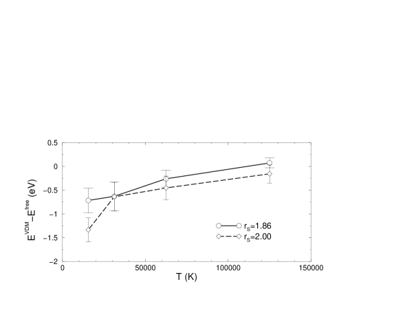
FIG. 1.: Difference in the internal energy from PIMC simulations with VDM and FP nodes vs. temperature using $N_{P}=32$ and $\tau^{-1}=2\cdot 10^{6}\rm{K}$.

Simulations with VDM nodes lead to lower internal energies than those with FP nodes as shown in Fig. 1. Since the free energy $F$ is the integral of the internal energy over temperature, one can conclude that VDM nodes yield to a smaller $F$ and hence, are the more appropriate nodal surface.

For the two densities considered here, the state of deuterium goes from a plasma of strongly interacting but un-bound deuterons and electrons at high $T$ to a regime at low $T$, which is characterized by a significant electronic degeneracy and bound states. Also at decreasing $T$, one finds an increasing number of electrons involved in long permutation cycles. Additionally for $T\leq 15\,625\,\rm{K}$, molecular formation is observed. Comparing FP and VDM nodes, one finds that VDM predicts a higher molecular fraction and fewer permutations hinting to more localized electrons.

III Shock Hugoniot

The recent experiments measured the shock velocity, propagating through a sample of pre-compressed liquid deuterium characterized by an initial state, ($E_{0}$, $V_{0}$, $p_{0}$) with $T=19.6\,\rm{K}$ and $\rho_{0}=0.171\,\rm{g/cm^{3}}$. Assuming an ideal planar shock front, the variables of the shocked material ($E$, $V$, $p$) satisfy the hugoniot relation [16],

$$H=E-E_{0}+\frac{1}{2}(V-V_{0})(p+p_{0})=0\quad.$$ (12)

We set $E_{0}$ to its exact value of $-15.886\rm{eV}$ per atom [17] and $p_{0}=0$. Using the simulation results for $p$ and $E$, we calculate $H(T,\rho)$ and then interpolate $H$ linearly at constant $T$ between the two densities corresponding to $r_{s}=1.86$ and $2$ to obtain a point on the hugoniot in the $(p,\rho)$ plane. (Results at $r_{s}=1.93$ confirm the function is linear within the statistical errors). The PIMC data for $p$, $E$, and the hugoniot are given in Tab. I.

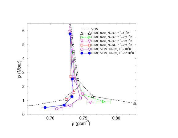
FIG. 2.: Comparison hugoniot function calculated with PIMC simulations of different accuracy: FP nodes with $N_{P}$=32 ($\triangle$ for $\tau^{-1}=10^{6}\rm K$ reported in [5], $\rhd$ for $\tau^{-1}=2\cdot 10^{6}\rm K$, $\bigtriangledown$ for $\tau_{F}^{-1}=8\cdot 10^{6}\rm{K}$ and $\tau_{B}^{-1}=2\cdot 10^{6}\rm{K}$) and $N_{P}$=64 ($\Box$ for $\tau^{-1}=2\cdot 10^{6}\rm{K}$) as well as with VDM nodes and $N_{P}$=32 ($\circ$ for $\tau^{-1}=10^{6}\rm{K}$ and $\bullet$ for $\tau^{-1}=2\cdot 10^{6}\rm{K}$). Beginning at high pressures, the points on each hugoniot correspond to the following temperatures $125\,000,62\,500,31\,250,15\,625,$ and $10\,000\,\rm{K}$. The dashed line corresponds to a calculation using the VDM alone.

In Fig. 2, we compare the effects of different approximations made in the PIMC simulations such as time step $\tau$, number of pairs $N_{P}$ and the type of nodal restriction. For pressures above 3 Mbar, all these approximations have a very small effect. The reason is that PIMC simulation become increasingly accurate as temperature increases. The first noticeable difference occurs at $p\approx 2.7\rm{Mbar}$, which corresponds to $T=62\,500\,\rm{K}$. At lower pressures, the differences become more and more pronounced. We have performed simulations with free particle nodes and $N_{P}=32$ for three different values of $\tau$. Using a smaller time step makes the simulations computationally more demanding and it shifts the hugoniot curves to lower densities. These differences come mainly from enforcing the nodal surfaces more accurately, which seems to be more relevant than the simultaneous improvements in the accuracy of the action $S$, that is the time step is constrained more by the Fermi statistics than it is by the potential energy. We improved the efficiency of the algorithm by using a smaller time step $\tau_{F}$ for evaluating the Fermi action than the time step $\tau_{B}$ used for the potential action. Unless specified otherwise, we used $\tau_{F}=\tau_{B}=\tau$. At even lower pressures not shown in Fig. 2, all of the hugoniot curves with FP nodes turn around and go to low densities as expected.

As a next step, we replaced the FP nodes by VDM nodes. Those results show that the form of the nodes has a significant effect for $p$ below 2 Mbar. Using a smaller $\tau$ also shifts the curve to slightly lower densities. In the region where atoms and molecules are forming, it is plausible that VDM nodes are more accurate than free nodes because they can describe those states [15]. We also show a hugoniot derived on the basis of the VDM alone (dashed line). These results are quite reasonable considering the approximations (Hartree-Fock) made in that calculation. Therefore, we consider the PIMC simulation with the smallest time step using VDM nodes ($\bullet$) to be our most reliable hugoniot. Going to bigger system sizes $N_{P}=64$ and using FP nodes also shows a shift towards lower densities.

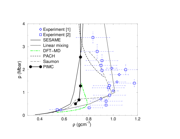
FIG. 3.: Comparison of experimental and several theoretical Hugoniot functions. The PIMC curve was calculated with VDM nodes, $\tau^{-1}=2\cdot 10^{6}\,\rm{K}$, and $32$ pairs of electrons and deuterons.

Fig. 3 compares the Hugoniot from Laser shock wave experiments [1, 2] with PIMC simulation (VDM nodes, $\tau^{-1}=2\cdot 10^{6}\,\rm{K}$) and several theoretical approaches: SESAME model by Kerley [3] (thin solid line), linear mixing model by Ross (dashed line) [4], DFT-MD by Lenosky et al. [8] (dash-dotted line), Padé approximation in the chemical picture (PACH) by Ebeling et al. [11] (dotted line), and the work by Saumon et al. [10] (thin dash-dotted line).

The differences of the various PIMC curves in Fig. 2 are small compared to the deviation from the experimental results [1, 2]. There, an increased compressibility with a maximum value of $6\pm 1$ was found while PIMC predicts $4.3\pm 0.1$, only slightly higher than that given by the SESAME model. Only for $p>2.5\rm Mbar$, does our hugoniot lie within experimental errorbars. In this regime, the deviations in the PIMC and PACH hugoniot are relatively small, less than $0.05\,\rm gcm^{-3}$ in density. In the high pressure limit, the hugoniot goes to the FP limit of 4-fold compression. This trend is also present in the experimental findings. For pressures below 1 Mbar, the PIMC hugoniot goes back lower densities and shows the expected tendency towards the experimental values from earlier gas gun work [18, 19] and lowest data points from [1, 2]. For these low pressures, differences between PIMC and DFT-MD are also relatively small.

IV Conclusions

We reported results from PIMC simulations and performed a finite size and time step study. Special emphasis was put on improving the fermion nodes where we presented the first PIMC results with variational instead of FP nodes. We find a slightly increased compressibility of $4.3\pm 0.1$ compared to the SESAME model but we cannot reproduce the experimental findings of values of about $6\pm 1$. Further theoretical and experimental work will be needed to resolve this discrepancy.

TABLE I.: Pressure $p$ and internal energy per atom $E$ from PIMC simulations with $32$ pairs of electrons and deuterons. For $T\geq 250\,000\,\rm{K}$, we list results from simulations with FP nodes and $\tau_{F}^{-1}=8\cdot 10^{6}\,\rm{K}$ and $\tau_{B}^{-1}=2\cdot 10^{6}\,\rm{K}$, otherwise with VDM nodes and $\tau^{-1}=2\cdot 10^{6}\,\rm{K}$.

$T(K)$	$p(Mbar),r_{s}=2$	$E(\rm{eV}),r_{s}=2$	$p(\rm{Mbar}),r_{s}=1.86$	$E(\rm{eV}),r_{s}=1.86$	$\rho^{Hug}(\rm{gcm}^{-3})$	$p^{Hug}(\rm{Mbar})$
1000000	53.79 $\pm$ 0.05	245.7 $\pm$ 0.3	66.85 $\pm$ 0.08	245.3 $\pm$ 0.4	0.7019 $\pm$ 0.0001	56.08 $\pm$ 0.05
500000	25.98 $\pm$ 0.04	113.2 $\pm$ 0.2	32.13 $\pm$ 0.05	111.9 $\pm$ 0.2	0.7130 $\pm$ 0.0001	27.48 $\pm$ 0.04
250000	12.12 $\pm$ 0.03	45.7 $\pm$ 0.2	14.91 $\pm$ 0.03	44.3 $\pm$ 0.2	0.7242 $\pm$ 0.0001	12.99 $\pm$ 0.02
125000	5.29 $\pm$ 0.04	11.5 $\pm$ 0.2	6.66 $\pm$ 0.02	11.0 $\pm$ 0.1	0.7300 $\pm$ 0.0003	5.76 $\pm$ 0.02
62500	2.28 $\pm$ 0.04	-3.8 $\pm$ 0.2	2.99 $\pm$ 0.04	-3.8 $\pm$ 0.2	0.733 $\pm$ 0.001	2.54 $\pm$ 0.03
31250	1.11 $\pm$ 0.06	-9.9 $\pm$ 0.3	1.58 $\pm$ 0.07	-9.7 $\pm$ 0.3	0.733 $\pm$ 0.003	1.28 $\pm$ 0.05
15625	0.54 $\pm$ 0.05	-12.9 $\pm$ 0.3	1.01 $\pm$ 0.05	-12.0 $\pm$ 0.2	0.721 $\pm$ 0.004	0.68 $\pm$ 0.04
10000	0.47 $\pm$ 0.05	-13.6 $\pm$ 0.3	0.80 $\pm$ 0.08	-13.2 $\pm$ 0.4	0.690 $\pm$ 0.007	0.51 $\pm$ 0.05

REFERENCES

- [1] I. B. Da Silva et al. Phys. Rev. Lett., 78:783, 1997.
- [2] G. W. Collins et al. Science, 281:1178, 1998.
- [3] G. I. Kerley. Molecular based study of fluids. page 107. ACS, Washington DC, 1983.
- [4] M. Ross. Phys. Rev. B, 58:669, 1998.
- [5] B. Militzer, W. Magro, and D. Ceperley. Contr. Plasma Physics, 39 1-2:152, 1999.
- [6] C. Pierleoni, D.M. Ceperley, B. Bernu, and W.R. Magro. Phys. Rev. Lett., 73:2145, 1994.
- [7] W. R. Magro, D. M. Ceperley, C. Pierleoni, and B. Bernu. Phys. Rev. Lett., 76:1240, 1996.
- [8] T. J. Lenosky, S. R. Bickham, J. D. Kress, and L. A. Collins. Phys. Rev. B, 61:1, 2000.
- [9] G. Galli, R.Q. Hood, A.U. Hazi, and F. Gygi. in press, Phys. Rev. B, 1999.
- [10] D. Saumon, G. Chabrier, and H. M. Van Horn. Astrophys. J., 99 2:713, 1995.
- [11] W. Ebeling and W. Richert. Phys. Lett. A, 108:85, 1985.
- [12] D. M. Ceperley. Rev. Mod. Phys., 67:279, 1995.
- [13] D. M. Ceperley. Monte carlo and molecular dynamics of condensed matter systems. Editrice Compositori, Bologna, Italy, 1996.
- [14] D. M. Ceperley. J. Stat. Phys., 63:1237, 1991.
- [15] B. Militzer and E. L. Pollock. in press, Phys. Rev. E, 2000.
- [16] Y. B. Zeldovich and Y. P. Raizer. Physics of Shock Waves and High-Temperature Hydrodynamic Phenomena. Academic Press, New York, 1966.
- [17] W. Kolos and L. Wolniewicz. J. Chem. Phys., 41:3674, 1964.
- [18] W.J. Nellis and A.C. Mitchell et al. J. Chem. Phys., 79:1480, 1983.
- [19] N.C.Holmes, M. Ross, and W.J.Nellis. Phys. Rev. B, 52:15835, 1995.