Measurement of mechanical vibrations excited in aluminium resonators by 0.6 GeV electrons.

NIKHEF 99-036 To be published by Review of Scientific Instruments, May 2000

Abstract

We present measurements of mechanical vibrations induced by 0.6 GeV electrons impinging on cylindrical and spherical aluminium resonators. To monitor the amplitude of the resonator’s vibrational modes we used piezoelectric ceramic sensors, calibrated by standard accelerometers. Calculations using the thermo-acoustic conversion model, agree well with the experimental data, as demonstrated by the specific variation of the excitation strengths with the absorbed energy, and with the traversing particles’ track positions. For the first longitudinal mode of the cylindrical resonator we measured a conversion factor of 7.4 $\pm$ 1.4 nm/J, confirming the model value of 10 nm/J. Also, for the spherical resonator, we found the model values for the $L$=2 and $L$=1 mode amplitudes to be consistent with our measurement. We thus have confirmed the applicability of the model, and we note that calculations based on the model have shown that next generation resonant mass gravitational wave detectors can only be expected to reach their intended ultra high sensitivity if they will be shielded by an appreciable amount of rock, where a veto detector can reduce the background of remaining impinging cosmic rays effectively.

04.80.Nn 07.07.Df 07.64.+z 07.77.Ka 29.40.Gx 29.40.Wk 43.20.Ks 43.35.Ud 95.55.Ym 96.40.Vw 96.40.z

1 Introduction

A key issue for a Resonant Mass Gravitational Wave Detector  [1] of improved sensitivity with respect to the existing detectors, is the background due to impinging cosmic ray particles [2, 3]. The energy deposited in the detector’s mass along a particle’s track may excite the very vibrational modes that are to signal the passing of a gravitational wave. Computer simulations of such effects are based on the thermo-acoustic conversion model and earlier measurements of resonant effects in Beron et al. [4] and Grassi Strini et al. [5]. According to the model, the energy deposited by a traversing particle heats the material locally around the particle track, which leads to mechanical tension and thereby excites acoustic vibrational modes [6]. At a strain sensitivity of the order of $10^{-21}$ envisaged for a next generation gravitational-wave detector, computer simulations  [3, 7] show that operation of the instrument at the surface of the earth would be prohibited by the effect of the cosmic ray background. Since the applicability of the thermo-acoustic conversion model would thus yield an important constraint on the operating conditions of resonant mass gravitational wave detectors, Grassi-Strini, Strini and Tagliaferri [5] measured the mechanical vibrations in a bar resonator bombarded by 0.02 GeV protons and 5*10^-4 GeV electrons. We extended that experiment by measuring the excitation patterns in more detail for a bar and a sphere excited by 0.6 GeV electrons. Even though we cannot think of a reason why the model, if applicable to the bar, would not hold for a sphere, we did turn to measuring with a sphere also.
We exposed [8] two aluminium 50ST alloy cylindrical bars and an aluminium alloy sphere, each equipped with piezoelectric ceramic sensors, to a beam of $\approx 0.6$ GeV electrons used in single bunch mode with a pulse width of up to $\approx 2\mu$s, and adjustable intensity of $10^{9}$ to $10^{10}$ electrons. We recorded the signals from the piezo sensors, and Fourier analysed their time series. Before and after the beam run we calibrated the sensor response of one of the bars for its first longitudinal vibrational mode at $\approx$ 13 kHz to calibrated accelerometers.

2 Experiment setup and method

In the experiment we used three different setups in various runs, as summarised in table I: two bars and a sphere. With the un-calibrated bar BU we explored the feasibility of the measurement. Also, bar BU proved useful to indirectly determine the relative excitation amplitudes of higher longitudinal vibrational modes, see sec. 4.1. With bar BC calibrated at its first longitudinal vibrational mode, we measured directly its excitation amplitude in the beam. Finally, with the sphere we further explored the applicability of the model.

Table I. Characteristics of our setup. Setup code name: BC BU SU Resonator type: bar bar sphere Diameter: 0.035 m 0.035 m 0.150 m Length: 0.2 m 0.2 m - Suspension: plastic string plastic string brass rod 0.15 m*0.002 m Piezo sensors: 1 2 2 Piezo hammer: 0 1 1 Capacitor driver 1 0 0 Direct calibration yes no no Beam energy 0.76 GeV 0.62 GeV 0.35 GeV Beam peak current 3 mA 18 mA 19 mA Electrons per burst $\approx 10^{9}$ $\approx 5\cdot 10^{10}$ $\approx 5\cdot 10^{10}$ Mean absorbed energy per electron 0.02 GeV 0.02 GeV 0.1 GeV Typical absorbed energy per burst 0.01 J 0.6 J 3.0 J

2.1 Electron beam

We used the Amsterdam linear electron accelerator MEA [9, 10] delivering an electron beam with a pulse-width of up to 2 $\mu$s in its hand-triggered, single bunch mode. The amount of charge per beam pulse was varied, recorded by a calibrated digital oscilloscope, photographed and analysed off line to determine the number of impinging electrons per burst.

2.2 Suspension and positioning

In both setups BC and BU, see fig. 1, the cylindrical aluminium bar was horizontally suspended in the middle, as indicated in the figure, with a plastic string.

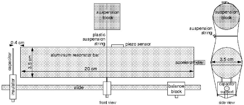
Figure 1: Calibrated bar setup BC. The beam traverses the bar’s front side perpendicular to the drawing plane.

The bar’s cylinder axis was positioned at 90⁰ to the beam direction. The bar’s suspension string was connected to a horizontally movable gliding construction, enabling us to handle the resonator by remote control, and let the impinging electron beam hit it at different horizontal positions. The aluminium sphere SU, see fig. 2, was suspended from its centre by a brass rod. Either the bar’s gliding construction, or the sphere’s suspension bar, was attached to an aluminium tripod mounted inside a vacuum chamber [9], which was evacuated to about $10^{-5}~{}$mbar. By remote control, we rotated the tripod and moved it vertically to either let the beam pass the resonator completely, or let it traverse the resonator. We let the beam traverse the sphere at different heights and different incident angles with respect to the piezo sensors positions on the sphere.

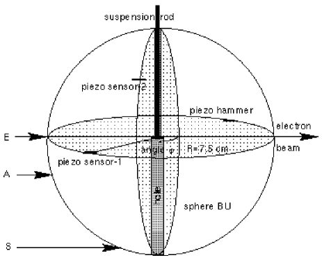
Figure 2: The spherical resonator setup, SU.

We mark the beam heights as E (Equator) and A (Africa) at 0.022 m below the equator. The E beam passed horizontally through the sphere’s origin, remaining in the same vertical plane for the A beam.

2.3 Sensors and signal processing

In setup BC we used a single piezo sensor of $\approx 15*3*1~{}$mm³ and glued it over it full length at 0.01 m off the centre on the top of the bar. Bar BC was equipped with a capacitor plate of 0.03 m diameter at a distance of $\approx 0.004$ m from one of its end faces. In setup BU one piezo sensor of $\approx~{}3*6*0.3~{}$mm³ was fixed on one end face of the bar.
A similar sensor of about the same dimensions was fixed in the same manner, oriented parallel to the cylinder’s long axis at a position 35 mm away from the end-face, In the third setup, SU, see fig. 2, two piezo sensors of $\approx~{}3*6*0.3~{}$mm³ were glued to the sphere’s surface. One was situated at the equator, with respect to the vertical rotation axis, the other one at a relative displacement of $45^{0}$ west longitude, and at $45^{0}$ north latitude.
For the setup in use, each sensor was connected to a charge amplifier of $\approx 2*10^{10}~{}$V/C gain. The signals were sent through a Krohn-Hite 3202R low-pass 100 kHz pre-filter, to a R9211C Advantest spectrum analyser with internal 2 MHz pre-sampling and 125 kHz digital low-pass filtering. The oscillation signals were recorded for 64 ms periods at a 4 $\mu$s sample rate. The beam pulse could be used as a delayed trigger to the Advantest. Using the memory option of the Advantest, the piezo signals were recorded from  0.3 ms onward before the arrival of the trigger. The data were stored on disk and were Fourier analysed off line.

2.4 Checks and stability

The data were taken at an ambient temperature of $\approx 23~{}^{0}$C. By exciting the resonator with the piezo-hammer we checked roughly its overall performance. As to be discussed in section 3, setup BC was calibrated before and after the beam run. The instrument’s stability was checked several times during the run by an electric driving signal on its capacitor endplate.

3 Calibration of bar BC’s piezo ceramic sensor

A standard accelerometer mounted on the bar damped the vibrations too strongly to confidently measure their excitations in the electron beam. Therefore the response of the piezoelectric ceramic together with its amplifier was first calibrated against two 2.4 gramme Bruel&Kjaer 4375 accelerometers glued, one at a time, to bar BC’s end face and connected to a 2635 charge amplifier. The resonator was excited through air by a nearby positioned loud-speaker driven from the Advantest digitally tunable sine-wave generator. The output signals from both the piezoelectric ceramic amplifier and the accelerometer amplifier were fed into the Advantest. Stored time series were read out by an Apple Mac 8100 AV, running Lab-View for on-line Fourier analysis, peak selection, amplitude and decay time determination.
We took nine calibration runs varying the charge amplifier’s sensitivity setting, and dismounting and remounting either of the two accelerometers to the bar. For the lowest longitudinal vibrational mode we calculated the ratio of the Fourier peak signal amplitudes, $R$, from the piezoelectric ceramic and accelerometer.
With the calibrated bar BC positioned in the electron beam line we checked the stability of the piezoelectric ceramic’s response intermittently with the beam runs by exciting the bar through its capacitor plate at one end face, electrically driving it at and around half the bar’s resonance frequency. We found the response to remain stable within a few percent.
After the beam runs we took additional calibration values in air with a newly acquired Bruel&Kjaer 0.5 g 4374S subminiature accelerometer and a Nexus 2692 AOS4 charge amplifier.

Figure 3: Response at the lowest longitudinal acoustic frequency of bar BC’s piezo (lower) and accelerometer (upper) Fourier amplitudes by constant amplitude loud-speaker driving. Left: on-resonance, $f$=12950 Hz. Right: slightly off-resonance, $f$=12850 Hz.

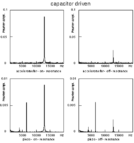
Figure 4: Response of bar BC’s piezo (lower) and accelerometer (upper) Fourier amplitudes by electrostatic capacitor plate driving. Left: on-resonance, $f$=6481.7 Hz. Right: slightly off-resonance, $f$=6480.0 Hz. The piezo peak of constant amplitude at 6.5 kHz arising from crosstalk is absent in the accelerometer, while the acoustic resonance is clearly seen at 13 kHz in both.

In fig. 3, typical frequency responses are shown when driving the bar by a loud-speaker signal. The upper part gives the Fourier peak amplitude of the bar’s 13 kHz resonance as measured with the accelerometer. The lower part gives the corresponding amplitude for the signal from the piezoelectric ceramic. The right hand side of the picture shows the amplitudes to be smaller, as expected when driving the bar slightly off resonance. We calculate the decay time, $\tau$, of the k-th mode amplitude $A_{k}(t)=A_{k}(0)\cdot e^{-t/\tau}$ to be $\tau=0.4$ s for this setup, equipped with the relatively light accelerometer.
Figure 4 shows the corresponding two signals when driving the bar by the capacitor plate at 6.5 kHz, that is at half the bar’s resonance frequency. Here, the direct electric response of the piezoelectric ceramic’s signal to the driving sine-wave is present, clearly without a mechanic signal, as would have shown up in the accelerometer. The direct signal at 6.5 kHz remains constant. On the other hand, the bar’s mechanical signals on and off its resonance frequency around 13 kHz show the expected amplitude change again, thereby demonstrating that around the bar’s resonance, the piezoelectric ceramic does only respond to the mechanical signal, not to the electric driving signal. See also the caption of fig. 4.

We calculated the average value of $R_{0}=V_{piezo}^{Fourier}/V_{accel.}^{Fourier}$ and the error over all 29 measurements, finding for the calibration factor at f=13 kHz,

$$\beta=R_{0}S(2\pi f)^{2}=(2.2~{}\pm~{}0.3)~{}\mbox{V/nm}$$ (1)

where $S=0.1~{}$V/ms^-2 is the amplifier setting of the accelerometer.

4 Beam experiments

Sensor signals way above the noise level were observed for every beam pulse hitting the sphere or the bar. We ascertained that: a) the signals arose from mechanical vibrations in the resonator, and b) they were directly initiated by the effect of the beam on the resonator, and not arising from an indirect effect of the beam on the piezo sensors. Our assertion is based on a combination of test results observed for both the bars and the sphere, as now to be discussed.

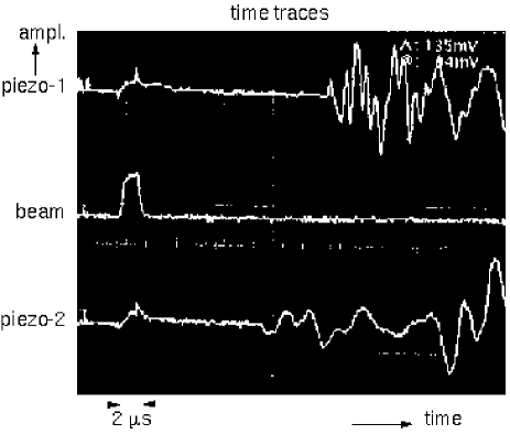
Figure 5: The $2~{}\mu$s electron bunch (middle trace) and the piezo sensors signals on the sphere (upper and lower traces).

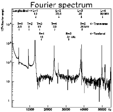
Figure 6: A typical Fourier spectrum of bar BC as excited by the electron beam. Data were analysed over 0.016 s duration, from 0.008 s onwards after the beam passed. Identified vibrational modes are indicated.

First, when the beam passed underneath the resonator without hitting it, we observed no sensor signal above the noise. Second, as shown in fig. 5, the sensors’ delayed responses after the impact of the beam agreed with the sound velocity. Here the beam was hitting the sphere at a position 5 mm above the sphere’s south pole. The middle trace shows the beam pulse of $\approx 2\mu$s duration. The two other traces show both piezo sensors to respond with a transient signal right from the start time of the beam’s arrival and to begin oscillating after some delay, depending on their distance from the beam. The distance of the equatorial sensor to the beam hitting the sphere at the south pole was 0.11 m, corresponding to $\approx 22~{}\mu$s travel time for a sound velocity of $\approx 5*10^{3}$ m/s. The signal is indeed seen in the lowest trace starting to oscillate at that delay time. The upper trace shows the signal from the second sensor situated on the northern hemisphere at 0.14 m from the traversing beam, correspondingly starting to oscillate with a delay of $\approx 28~{}\mu$s after the impact of the beam. Third, after dismounting the piezo-hammer from the resonator, we observed that the sensor signals did not change, which showed that the activation is not caused by the beam inducing a triggering of the piezo-hammer. Fourth, to simulate the electric effect of the beam pulse on the sensors, we coupled a direct current of 60 mA and 2.5 $\mu$s duration from a wave packet generator to the bar. Apart from the direct response of the piezo-sensor during the input driving wave, no oscillatory signal was detected above the noise level. Finally, we measured the dependence of the amplitudes in several vibrational modes on the hit position of the beam, as will be described in the following sections. We found the amplitudes to follow the patterns as calculated with the thermo-acoustic conversion model.

4.1 Results for the bar

In fig. 6 a typical Fourier spectrum of bar BC is shown up to 55 kHz. The arrows point to identified vibrational modes [11]. From a fit of $K$ and $f_{0}$ of the longitudinal frequencies $f_{L}=L\cdot f_{0}\cdot(1-L^{2}K)$ [12] of the modes for $L$=1,..,4, we find $f_{0}=12933,K=0.0022$, where $f_{0}$ is related to the sound velocity by $v_{s}=2l*f_{0}=5173$ m/s for our bar length of $l$=0.2 m. For the Poisson-ratio $\sigma=2l\surd K/(\pi r)$, $r$ being the cylinder radius of the bar, from our fit we get $\sigma=0.338$. The values agree well with the handbook [13] quoting $\sigma$=0.33 and $v_{s}$=5000 m/s for aluminium. The root mean square error of the fit is 35 Hz, in correspondence with the 30 Hz frequency resolution used in the Fourier analysis. Other peaks correspond to torsional and transverse modes [11, 12].

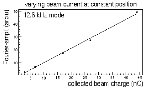
Figure 7: Correlation between the Fourier amplitude of the 12.6 kHz vibrational mode and the beam charge. Data points (*) and straight line fit.

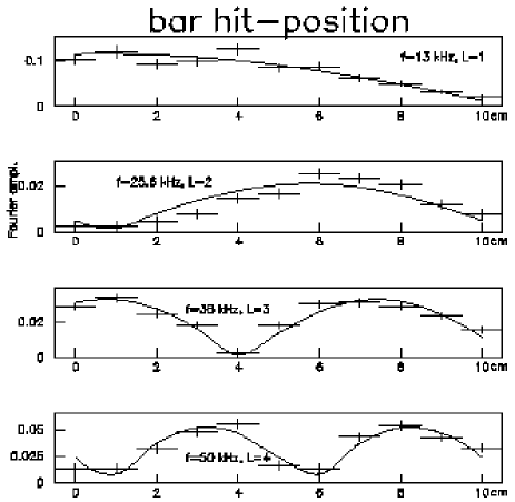
Figure 8: The measured, unnormalised Fourier amplitudes ($+$) and model calculations (–) as a function of the beam hit position along the cylinder axis for the four lowest longitudinal modes of bar BC.

The Fourier amplitudes $A_{k}$ of $f(t)=\sum A_{k}e^{i\omega_{k}t}$ of the modes depend linearly (as shown for the 13 kHz, $L$=1 mode in fig. 7) on the integrated charge in the beam pulse for a fixed beam position, and therefore also linearly on the energy deposited by the beam, which ranged in these runs from 0.06-0.8 J. The spread in the ratios of the amplitudes to the beam charge, shows the Fourier amplitudes to reproduce within $\pm~{}10\%$.

The agreement of the model to within 10% with the measured data is shown in fig. 8. The figure shows the measured Fourier amplitudes of bar BC at the piezo sensor and the calculations following Grassi Strini et al. [5, 14] as a function of the hit position along the cylinder axis for the first four longitudinal modes. For each mode the average model value was scaled to the average measured value. The best fit was found with a shift of the hit positions along the bar, by an overall offset of $x_{0}$=-0.0075 m, which corresponds to the crude way we aligned the bar with the beam line.

4.1.1 Lowest bar mode excitation amplitude

For the 13 kHz, $L$=1 mode we determine the absolute amplitude for a comparison with the model calculation of ref. [5, 14]. Firstly, we use the amplitude function B₀(x), see eq. 9 of ref. [5, 14], by rewriting it in the form:

$$B_{0}(x)=2\cdot\kappa_{0}\cdot\Delta E/\pi\times cos(\pi x/l)sin(\pi\eta/(2l))/\pi\eta/(2l)$$ (2)

with

$$\kappa_{0}=\alpha\cdot l/(c_{v}\cdot M)=\alpha/(c_{v}\cdot\rho O).$$ (3)

In this expressions $x$ is the hit position along the the cylinder axis, $l$ the bar length, $\eta$ the beam diameter, $\alpha$ the thermal linear expansion coefficient, $\rho$ the density, c_v the specific heat, $O$ the cylindrical surface area of the bar, and $\Delta E$ the energy absorbed by the bar. From $B_{0}(x)$ we derive the functional form for the measured values of $W_{sens}$ as

$$W_{sens}(x)=\frac{B_{0}(x)}{\Delta E}\beta D\frac{dE}{dQ}$$ (4)

where $dE/dQ$ is the beam energy absorbed by the bar per unit of impinging beam charge, $\beta$ the calibration factor as discussed in section 3, and D the decay factor $e^{-t/\tau}$, since eq. 2 applies at excitation time and we have to correct the amplitude at measuring time for the mode’s decay, corresponding to its Q-factor. Therefore,

$$W_{sens}(x)=\kappa_{exp}2/\pi\times cos(\pi x/l)sin(\pi\eta/(2l))/\pi\eta/(2l),$$ (5)

with

$$\kappa_{exp}=\beta D\kappa_{0}\frac{dE}{dQ}$$ (6)

From fitting eq. 5 to the measured values $W_{sens}(x)$ given in table II with $\kappa_{exp}$ as the free variable, we find our presently measured value for $\kappa_{0}^{exp}=\kappa_{exp}\cdot/(dE/dQ\cdot D\cdot\beta)$ which we compare to the model value in eq. 3. Secondly, the decay time was measured by recording the sensor signals after a trigger delayed by up to 1.6 s at a fixed beam hit position. An exponential fit $A(t)=A_{0}*e^{-t/\tau}$ to the mode amplitude gives $\tau=(0.36\pm 0.01)~{}$s for the $L$=1 mode. This corresponds to a Q-value of $\approx$ 15000, a value consistent with the room temperature measurement of aluminium as in ref. [15], and indicating a negligible influence of the suspension and piezoelectric ceramic sensor for this mode. From the measured value of $\tau$ and a mean delay time from the start of the beam pulse of 0.016 s, we calculate the decay factor to be $D=0.95$.

Table II. Excitation values W_sens, equalling the ratio of the measured Fourier amplitude and the measured beam pulse charge at each of the indicated hit positions on the bar for the 13 kHz, $L$=1 mode.

hit position $x$ cm	0	1	2	3	4	5	6	7	8	9	10
Wsens V/nC	0.185	0.216	0.167	0.180	0.225	0.152	0.152	0.157	0.112	0.089	0.057

Thirdly, as indicated, we use the data for W_sens in the second row of table II to fit the variable $\kappa_{exp}$ in eq. 5, where now x is the hit position as given in row 1, $l$=0.2 m , and $\eta=0.002$ m. The value found in the fit is $\kappa_{exp}=(0.300\pm 0.025)$ V/nC. Fourthly, from a Monte Carlo simulation at the beam energy of 570 MeV used for these runs, we calculate the mean absorbed energy and the mean energy spread which results from the fluctuating energy losses of the passing electrons and the energies of the secondaries escaping from the bar, as $\Delta$E_e=(19$\pm$ 2) MeV. The electron beam pulse thus deposits $dE/dQ=(0.019\pm~{}0.002)$ J/nC in the bar. Using the measured calibration value at f=12986 Hz as given in eq. 1, $\beta$=(2.2 $\pm$ 0.3) V/nm, we arrive at

$$\kappa^{exp}_{0}=(7.4\pm~{}1.4)~{}\mbox{nm/J}.$$ (7)

Finally, we calculate the model value of $\kappa_{0}$ from the material constants as being $\kappa_{0}$=10 nm/J, neglecting the much smaller error as arising from some uncertainty in the parameters. We conclude that $\kappa^{exp}_{0}/\kappa_{0}=(0.74\pm 0.14)$, a result that is consistent with the validity of the model of ref. [5, 14].
The measured maximum excitation amplitude at beam position $x$=0, see fig. 8 for the 13 kHz, $L$=1 longitudinal mode thus corresponds to (0.13 $\pm$ 0.02) nm.

4.1.2 Higher bar mode excitation amplitudes

Having determined the correspondence between the model calculation and the experiment’s result for the first longitudinal vibrational mode amplitude, we return to some of the higher vibrational modes. To compare the modes we need to take the sensor position on the bar into account. We rewrite the displacement amplitude of eq. 5 from ref. [5] as a function of hit position $x_{h}$ and sensor position $x_{s}$ as:

$$\Phi_{odd-L}=(2\kappa/L\pi)sin(L\pi x_{s}/l)cos(L\pi x_{h}/l),$$

$$\Phi_{even-L}=(2\kappa/L\pi)cos(L\pi x_{s}/l)sin(L\pi x_{h}/l),$$ (8)

where $l$ is the bar length. We dropped the beam width correction term which would lead to a less than 0.1% correction even for $L$=4. We approximate the sensor response by the local strain along bar BC’s cylinder axis, that is to the d$\Phi$/dx_s of eq. 8, arriving at a sensor response, S_L:

$$S_{odd-L}=B_{L}cos(L\pi x_{h}/l),B_{odd-L}=(2\epsilon\kappa/l)cos(L\pi x_{s}/l),$$

$$S_{even-L}=B_{L}sin(L\pi x_{h}/l),B_{even-L}=(2\epsilon\kappa/l)sin(L\pi x_{s}/l),$$ (9)

where $\epsilon$ is a sensor response parameter. The $x_{s}$ dependent term did not enter into the calculation of $\kappa_{0}^{exp}$ in the previous section, since the calibration was done at the same sensor position as the beam measurement. However, for a comparison between the modes, the dependence on the sensor position $x_{s}$ has to be taken into account. Since the variables are strongly correlated, we, first, fitted for each mode the term $B_{L}$ in the $x_{h}$ dependent part of eq. 9 to the measured value of $W_{sens}$ for the mode, shifting the origin of $x_{h}$ by 0.0075 m, as mentioned before. The results are given in the first row of table III.

Table III. Bar BC modes comparison. The piezoelectric ceramic sensor responds to the bar’s strain.

description	symbol	13 kHz,$L$=1	25.6 kHz,$L$=2	38 kHz,$L$=3	50 kHz,$L$=4
amplitude	$B_{L}^{meas}$	0.12$\pm 0.01$	0.021$\pm 0.002$	0.033$\pm 0.03$	0.052$\pm 0.005$
decay correction	D	1.04$\pm$0.001	1.17$\pm 0.02$	1.49 $\pm$0.06	1.14$\pm$0.01
$B_{L}^{meas}\times D$	$B_{L}^{exp}$	0.12$\pm 0.01$	0.025$\pm 0.003$	0.049$\pm 0.005$	0.059$\pm 0.006$
sensor position factor	$P_{L}$	1.02	2.61	1.20	1.41
$\epsilon\kappa 2/l=B_{L}^{exp}\times P_{L}(arb.u.)$	$\kappa^{\prime}$	0.12$\pm 0.01$	0.065$\pm 0.007$	0.059$\pm 0.006$	0.083$\pm 0.008$

Second, we corrected the amplitudes $B_{L}^{meas}$ for the mode decay with a factor $D$, given in row 2, and corresponding to the times $\tau_{1}=0.36~{}s,\tau_{2}=0.10~{}s,~{}\tau_{3}=0.04~{}s,~{}\tau_{4}=0.12~{}s$, which leads to the values of $B_{L}^{exp}$ in row 3. Finally, we multiplied with the factor $P_{odd-L}=1/cos(L\pi x_{s}/l)$, $P_{even-L}=1/sin(L\pi x_{s}/l)$, where the bar length is $l$=0.2 m. Since the sensor extends from 0.005 through 0.020 m from the center of the bar, we use the mean sensor position $x_{s}=0.0125$ m. The resulting values of $\kappa^{\prime}=2\epsilon\kappa/l$, shown in the last row, should be independent of L. For $L$=2,3,4 they are rather closely scattered around a mean value of $\kappa^{\prime}=0.07$ which is, however, at about half the $L$=1 value. This discrepancy might have originated from some resonances of the sensor itself, and we suspect the strong peak at 23 kHz, shown in figure 6, to be an indication of such resonances playing a role.
Since the amplitudes of the higher modes for bar BC do not comply with our expectations we turn, as a further check, to our un-calibrated measurements with bar BU. It had been equipped with a piezoelectric sensor at one end face where the longitudinal modes have maximum amplitude. The sensor had been mounted flatly with about half of its surface glued to the bar, and responding to the bar’s surface acceleration, not its strain as at bar BC. We extract the $\kappa_{L}$ values from our measurement analogously as for bar BC, following again the model calculations of Grassi Strini et al. [5], using the $L$=1 mode as the reference. The results are given in table IV.

Table IV. Bar BU modes comparison. The piezoelectric ceramic sensor responds to the bar’s acceleration. The value of $\kappa_{1}^{meas}$ for the $L$=1, 13 kHz mode is used as the reference for the higher modes.

description	symbol	13 kHz,$L$=1	25.6 kHz,$L$=2	38 kHz,$L$=3	50 kHz,$L$=4
relative amplitude	$B^{meas}$	1	1.15	11.5	3.6
relative decay correction	D	1	3$\pm$1	0.7$\pm$0.2	1.3$\pm$0.9
$(\omega_{L=1}/\omega_{L})^{2}$	$\Omega$	1	0.26	0.12	0.07
$B^{meas}\times D\times\Omega$	$\kappa^{meas}_{L}/\kappa^{meas}_{1}$	${\bf 1}$	0.8$\pm$0.3	0.9$\pm$0.4	0.3$\pm$0.3

After applying the decay correction factor $D$ and the frequency normalisation factor $\Omega$, the results should be independent of L. The $L$=4 value is significantly low, which, again, might be due to some interfering resonance. The $L$=2 and $L$=3 values, however, do not significantly deviate from the $L$=1 value, thus confirming the model calculations for these higher modes too.

4.2 Results for the sphere

Our measurements on the sphere consisted of a) hitting the sphere with the beam at one of two heights in the vertically oriented plane through its suspension: at the equator (E) and at 0.022 m southward (A); b) rotating the sphere with its two fixed sensors over $180^{0}$ around the suspension axis at each beam height, and measuring several times back and forth by steps of $30^{0}$ to diminish the influence of temperature and beam fluctuations, ending up on a $10^{0}$ angular lattice.

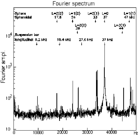
Figure 9: The Fourier amplitude spectrum of the sphere SU averaged over all measured angles for sensor-1, at beam height position E. The modes and frequencies as calculated, are indicated.

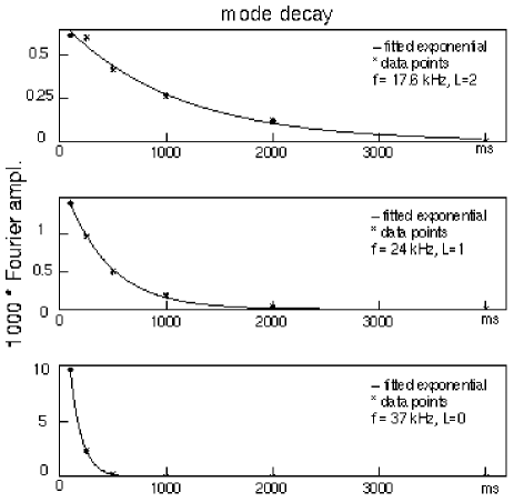
Figure 10: Decay of sphere’s vibrational modes as measured with delayed data taking of the spectrum analyser. The curve shows the fit of $A(t)=A_{0}*e^{-t/\tau}$. Upper: 17.6 kHz, $L$=2, $\tau$=1.1 s. Middle: 24 kHz, $L$=1, $\tau$=0.4 s. Lower: 37 kHz, $L$=0, $\tau$=0.1s.

The Fourier amplitude spectrum of sensor-1, averaged over the angular positions, is shown in fig. 9. The lowest spheroidal mode is most relevant for a spherical resonant mass gravitational wave detector, and we therefore focus on a few spheroidal modes. As expected, the lowest spheroidal $L$=2 mode is seen at 17.6 kHz, the lowest spheroidal $L$=1 mode at 24 kHz, and the lowest spheroidal $L$=0 mode at 37 kHz. Some other peaks are also indicated in the figure, though not the toroidal modes, which we neglect completely. It should be noted that while the $L\neq$0 amplitudes oscillate over the angles, the $L$=0 amplitude does not, leading to a relative enhancement of the latter in the angle-averaged fig. 9.
The Fourier amplitudes, again, showed a linear dependence on the deposited energy.
To determine the decay times at $f$=17.6, 24 kHz and 37 kHz, see fig. 10, we took data with up to 4 s delay in the spectrum analyser, and found $\tau\approx 1~{}$s, 0.4 s and 0.1 s respectively.

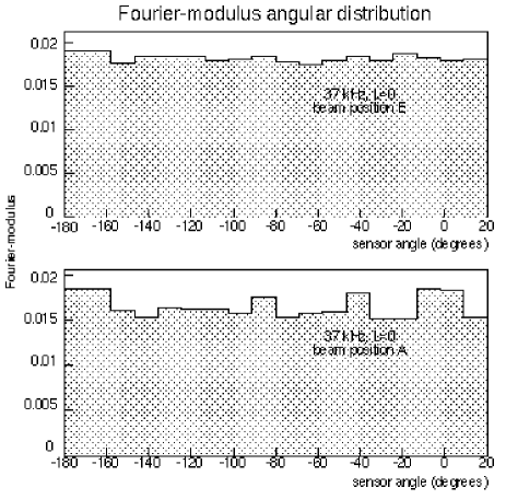
Figure 11: 37 kHz Fourier-modulus angular distribution. The beam hits the sphere at upper: E, lower: A.

The angular distributions for the amplitude of the 37 kHz, $L$=0 mode at the two vertical beam positions E and A are shown in figures 11. The $L$=0 amplitude is independent of the angle, and since the amplitude is constant to within 20% we infer from the Fourier-modulus’ deviation from flatness a 20% variation of the beam intensity from one shot to another.
During our measurement with the sphere we were unable to use the beam pulse as a trigger, implying that the start time of data acquisition with respect to the beam pulse is unknown. In our further analysis we will therefore use only the Fourier modulus, and not analyse the phases.
The absolute scale of the 37 kHz Fourier amplitude turned out to be $\approx 5$ times larger than the model value for sensor-2 and $\approx 50$ times for sensor-1. We assume this discrepancy to be based on some interference effects, possibly with a sensor resonance and a suspension bar mode, and we do not further analyse the $L$=0 mode. To disentangle the angular distributions in general, we felt, would squeeze the results of our simple measurement too much, for a couple of reasons. First, the Fourier amplitude $A_{L}$ for any multi-pole order $L$ in the sphere’s case is actually a sum of $M$-submodes. Though they would be degenerate for an ideal sphere, in practice some $M$-modes might or might not turn out to be split beyond the frequency-resolution of $\Delta f$=30 Hz. Second, both sensors $s_{1},s_{2}$ should be taken to have unknown sensitivities, e${}_{s_{j}}$, in three orthogonal directions, with phase factors +1 or -1 for their orientation. Third, though each mode would start to be excited within the same sub-nanosecond time interval of the beam crossing, the building up of each mode’s resonance vibration may lead to a specific phase $t^{0}_{M_{L},b_{k}}$ depending on the mode’s spatial relation to the beam path.
We now show that the calculated angular distributions have the signature of the $L$-character of the measurement. Therefore, we write the Fourier modulus at different impinging beam positions $b_{k}$ as a function of the angle $\phi$ as:

$$A_{L,s_{j},b_{k}}(\phi)=\mid F_{L,s_{j},b_{k}}~{}\mbox{\boldmath$\epsilon_{s_{j}}$}\cdot\sum_{-M_{L}}^{+M_{L}}s_{L,M_{L},b_{k}}{\bf u}_{L,M_{L},s_{j},b_{k}}(\phi)e^{\omega_{L}t^{0}_{M_{L},b_{k}}}\mid,$$ (10)

where $F_{L,s_{j},b_{k}}$ is a frequency response function for each sensor, which may depend also on the beam position. This normalisation factor is expected to be of order 1, and is kept fixed at 1 for the $L$=2 distributions. It is used as a free parameter for the $L$=1 distributions to compensate for the rather inaccurate knowledge of a) the sensor positions on the sphere’s surface, b) the beam track location and c) the electrons and photons shower development along the track, since the exact excitation strengths of the modes are quite sensitive to such data. As the first step in the fitting procedure we separately calculated the $s_{L,M_{L},b_{k}}{\bf u}_{L,M_{L},s_{j},b_{k}}$, where $s_{L,M_{L},b_{k}}$ is the mode’s strength from the beam excitation, as detailed in the appendix. We inserted the calculated $s_{L,M_{L},b_{k}}{\bf u}_{L,M_{L},s_{j},b_{k}}$ in a hierarchical fitting model, to simultaneously fit [16] the relevant parameters of eq. 10 to the 17.6 kHz, $L$=2 Fourier modulus $A_{L,s_{j},b_{k}}$ for both sensors $s_{1}$ and $s_{2}$ at both beam positions E and A. This fit led to a reduced $\chi^{2}$=1.3 at 59 degrees of freedom. Next, with fixed values for the sensor efficiencies $\epsilon_{s_{j}}$ so established, we fitted the relevant parameters for the 24 kHz, $L$=1 Fourier peaks, including the $L$=1 sensor response factors $F$. At all stages the $\mid t^{0}_{M_{L},b_{k}}\mid$ of the phases were kept within the bounds of the period of mode-$L$. With an uncertainty in the beam charge and in the Fourier peak amplitudes of $\approx 20\%$ each, the error amounts to $\approx$30%, and we took a minimum absolute error of 2$\times 10^{-5}$ for sensor $s_{1}$ and 1$\times 10^{-5}$ for sensor $s_{2}$. In total we have 152 data points, while the total number of fitted parameters is 27, including a relative normalising factor for the mean beam current at beam position A with respect to the mean current at beam position E. We found for the total fit a reduced $\chi^{2}$=1.6 at 125 degrees of freedom. The $L$=1 response factors remain within 1.1 and 0.2.

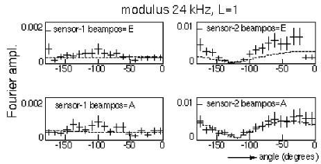
Figure 12: Data points (+) and fit results (—) for the sphere’s 24 kHz, $L$=1 mode. Left column: sensor-1, right colum: sensor-2. Upper row: beam position E, lower rows: beam position A. The x-axes give the angle of sensor-1. Note that the y-scales are different for the two sensors.

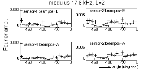
Figure 13: Data points (+) and fit results (—) for the sphere’s 17.6 kHz, $L$=2 mode. Left column: sensor-1, right colum: sensor-2. Upper row: beam position E, lower rows: beam position A. The x-axes give the angle of sensor-1. Note that the y-scales are different for the two sensors.

The results of the fits to the 17.6 kHz and 24  kHz are given in figures 12 and 13 and table V. Note the different vertical scales used for sensor-1 and sensor-2 in both pictures. Some of the parameters given in the table are strongly correlated.

Table V. Results of a hierarchical fit to the data of the sphere at the 19 measuring angles of both sensors $s_{1}$ and $s_{2}$ of the Fourier modulus at 17.6 kHz and 24 kHz at beam positions E and A.

sensor efficiency	fit result	error
	$*10^{-4}$ V/ms-2	$*10^{-4}$ V/ms-2
$\epsilon_{s_{1}}-r$	+0.10	0.02
$\epsilon_{s_{1}}-\theta$	-0.5	0.2
$\epsilon_{s_{1}}-\phi$	+0.4	0.1
$\epsilon_{s_{2}}-r$	-0.5	0.2
$\epsilon_{s_{2}}-\theta$	-0.5	0.2
$\epsilon_{s_{2}}-\phi$	+4.0	0.3
$intensity(\frac{beamA}{beamE})$	0.7	0.1
response factor
$F_{L=1,s_{1},beamA}$	0.3	0.1
$F_{L=1,s_{2},beamA}$	1.1	0.1
$F_{L=1,s_{1},beamE}$	0.2	0.1
$F_{L=1,s_{2},beamE}$	1.1	0.2

We conclude that the measured Fourier amplitude angular distributions are consistent with the model value for the $L$=2 and $L$=1 mode signature.

4.2.1 The sphere’s absolute displacement

Finally, to estimate the order of magnitude of the sphere’s absolute displacement, we have to take an intermediate step by first normalising bar BU to the calibrated results for bar BC and then use bar BU as a calibration for the sphere. The sensors used on bar BU consisting of the same sensor material and having been cut roughly to the same size, we assume to be identical to the ones used on sphere SU. The amplifiers used are identical. The bar BU sensors, however, differ strongly from those of bar BC.
We arrive at an indirectly calibrated value for $\epsilon_{BU,2}=(3.4*10^{-4}\pm 30\%)$ V/ms^-2 of sensor-2 on bar BU. The value of $\epsilon_{BU,1}$ for sensor-1 is about ten times smaller.
Then, for the sphere, the fitted value of $\epsilon_{s_{j}}$ given in table V, shows the largest value of sensor-2, $\epsilon_{\phi-SU}=(4*10^{-4}\pm 10\%)~{}$V/ms^-2, to lead to a ratio $\approx(1.2\pm 0.4)$ with $\epsilon_{BU}$. Again, the values for sensor-1 are about ten times smaller. The error of $\approx 33\%$ is the propagated statistical error only. The result seems reasonable. So, the model calculation and our sphere measurement results are of the same order of magnitude on an absolute scale too.
From the maximum Fourier modulus, $V^{max}=(0.003\pm 0.001)$ V, of the 17.6 kHz, $L$=2 sphere mode measured in sensor sensor-2 as given in fig. 13, and the absorbed energy of 3.1 J, we find the maximum sphere’s displacement to correspond to $(0.2\pm 0.1)$nm/J.

5 Discussion

Having confirmed the thermo-acoustic conversion model in the present experiment, we discuss some points about extrapolating these results to the actual operation of a resonant gravitational wave detector. Firstly, in our experiment many incident particles deposited their energy in the resonator, in contrast to a single muon hitting an actual detector. However, from this difference it seems unlikely to reach different conclusions, especially since in the process of depositing energy along its track, the muon will generate lots of secondary particles too. Also, we measured at room temperature while actual detectors would have to operate in the millikelvin range. An aluminium resonator, for instance, at such a temperature, would be superconducting, and it is as yet unclear how the decoupling of the electron gas from the lattice would affect the process of acoustic excitation.
Therefore, we hold it of particular importance for the prospected shielding of a next generation resonant mass gravitational wave detector that an existing millikelvin detector like the Nautilus [17, 18], would succeed in measuring the impinging cosmic rays in correlation with the resonator mode. Such a result, as a test for the further applicability of the thermo-acoustic conversion model at operating temperature, would come closest to the real situation envisaged for the new detectors.
Apart from such temperature effects, the applicability of the thermal acoustic conversion model [4, 5, 14] is confirmed by the data and therefore cosmic rays should be expected to seriously disrupt, as calculated by the model, the possibility of detecting gravitational waves. It is beyond the scope of this article to go into any detail [19]. We want to point, however, to earlier calculations [3, 7, 20] which, having used the model, clearly show, firstly, that a next generation spherical resonant mass gravitational wave detector of ultra high sensitivity will be significantly excited by cosmic rays. Secondly, the high impact rate of cosmic rays will prohibit gravitational wave detection at the earth’s surface, with the required sensitivity.
Finally, shielding the instrument by an appreciable layer of rock as available in, for instance, the Gran Sasso laboratory, would suppress the cosmic ray background by a factor of $\geq 10^{6}$. Even then a vetoing system will be necessary and, at the radical reduction of the background rate so established, it may indeed work effectively.

Appendix: Sphere excitation model calculation

Our calculation of the ($L,M$)-mode excitation strengths is based on the source term of eq. 5.10/11 of ref. [14], $s=\Sigma/(\rho V)*\int dz\nabla_{\perp}\cdot{\bf u}$, with $\Sigma=\gamma dE/dz$. Here, $\gamma$ is the Grueneisen constant, $\rho V$ de sphere’s mass, and $dE/dz$ the absorbed energy per unit track length. The Fourier amplitudes, measuring the second time derivative of the mode amplitudes, are directly proportional to $s$, and the mode amplitudes follow from $s/\omega^{2}$, as in eq. 5.18 of [14]. However, the amount of energy absorbed per unit length in our case depends on the particle’s position along the track. We therefore re-included the $\Sigma$-term under the source term’s integral by letting $dE(z)/dz$ represent the electromagnetic cascade development of ref. [21] as an approximation to the amount of energy absorbed per unit track length by the sphere at position z along the beam track,

$$s_{L,M_{L}}=\kappa\int_{L}{\bf\nabla}_{\bot}\cdot{\bf u}_{L,M_{L}}(z)\frac{dE(z)}{dz}dz,$$ (11)

where $z$ is being measured from the beam’s entrance point into the sphere. With $E_{abs}$ being the total amount of energy absorbed by the sphere from the electron bunch, we write $dE(z)/dz=E_{abs}*d(E(z)/E_{abs})/dz$ and use the polynomial expansion $d(E(z)/E_{abs})/dz=\sum_{i=0}^{3}c_{i}z^{i}$. Then $\int_{z_{min}}^{z_{max}}dzd(E(z)/E_{abs})/dz$=1. For the polynomial, measuring $z$ in meter, we acquired the values $c_{0}$=0.8332 m^-1, $c_{1}$=226 m^-2, $c_{2}$=-1832 m^-3, $c_{3}$=4909 m^-4 from a fit to the form given in ref. [21], with less than a percent deviation for our case of $0\leq z\leq 0.15$ m. The value for the energy absorbed by the sphere from a single electron, $E_{abs}^{e}$=123 MeV, we got from both our Monte Carlo simulation using GEANT [22], and from EGS4 [23, 24]. At the measured 25 nC beam pulse charge this corresponds to a total $E_{abs}=3.1~{}$J absorbed by the sphere. Then the value of $\kappa~{}E_{abs}=\gamma E_{abs}/M$=1.00 m²/s², for our case of $M=\rho V$=4.95 kg and $\gamma$=1.6. Our sphere has a suspension hole which leads to a slight shift in the frequencies and the spatial distribution of the modes, with respect to those of a sphere without a hole [25]. We approximated, however, our sphere’s modes by the ideal hole-free sphere’s eigenmode solutions u($z$) [26], using the available computer code as established in ref. [27], and renormalising to $\int{\bf u}\cdot{\bf u}dV=V$, as used in ref. [14] from eq. 5.6 onward. The source term $s_{L,M_{L}}$ was calculated for each mode ($L,M$) by numerically integrating eq. 11. We checked the surface term in the numerical procedure to be negligible, as assumed in the partial integration leading to the form of $s$ used by ref. [14]. Each u($\phi$) in eq. 10 is the eigenmode solution, calculated for each sensor on the $\phi$-grid of the measured data, and each term $s_{L,M_{L},b_{k}}$ is the excitation factor $s_{L,M_{L}}$ at the specific beam position $b_{k}$.

References

-
[1]
P. Astone, G.V. Pallottino, M. Bassan, E. Coccia, Y. Minenkov, I. Modena,
A. Moleti, M.A. Papa, G. Pizzella, P. Bonifazi, R. Terenzi, M. Visco,
P. Carelli, V. Fafone, A. Marini, S.M. Merkowitz, G. Modestino, F. Ronga,
M. Spinetti, L. Votano,
in:
p. 551 in: E. Coccia, G. Pizzella, G. Veneziano (eds.),
Proc. 2nd Amaldi conf. on
Gravitational Waves, CERN 1997, World Scientific 1999.
C. Frajuca, N.S. Magalh es, O.D. Aguiar, N.D. Solomonson, W.W. Johnson, S.M. Merkowitz and W.O. Hamilton, in: Proc. OMNI-I(1996), World Scientific 1997,
G.M. Harry, T.R. Stevenson, H.J. Paik, Phys.Rev.D54(1996)2409
C. Zhou, P.F. Michelson, Phys.Rev.D51(1995)2517.
GRAIL, NIKHEF, Amsterdam, May 1997.
G.D. van Albada, W. van Amersfoort, H. Boer Rookhuizen, J. Flokstra, G. Frossati, H. van der Graaf, A. Heijboer, E. van den Heuvel, J.W. van Holten, G.J. Nooren, J.E.J. Oberski, H. Rogalla, A. de Waele, P.K.A. de Witt Huberts, in Proc. Second Workshop on Gravitational Wave Data Analysis, pag. 27, Editions Frontières, 1997. -
[2]
F. Ricci, Nucl.Instr. and Meth. A260(1987)491,
J. Chang, P. Michelson, J. Price, Nucl.Instr. and Meth. A311(1992)603 - [3] G. Mazzitelli, M.A. Papa, Proc. OMNI-I(1996), World Scientific 1997
-
[4]
B.L. Beron, R. Hofstadter, Phys.Rev.Lett. 23,4(1969) 184,
B.L. Beron, S.P. Boughn, W.O. Hamilton, R. Hofstadter, T.W. Martin, IEEE Trans.Nucl.Sc. NS17(1970)65. - [5] A.M. Grassi Strini, G. Strini, G. Tagliaferri, J.Appl.Phys. 51,2(1980)948,
-
[6]
For non-resonant thermo-acoustic effects see for instance
I.A. Borshkoysky, V.V. Petrenko, V.D. Volovik, L.L. Goldin, Ya.L. Kleibock,
M.F. Lomanov, Lett.Nuovo Cimento 12(1975)638
L. Sulak, T. Armstrong, H. Baranger, M. Bregman, M. Levi, D. Mael, J. Strait, T. Bowen. A.E. Pifer, P.A. Polakos, H. Bradner, A. Parvulescu, W.V. Jones, J. Learned, Nucl.Instr. and Meth. 161(1979)203
J.G. Learned, Phys.Rev.D 19,11(1979)3293
G.A. Askariyan, B.A. Dolgoshein, A.N. Kalinovsky, N.V. Mokhov, Nucl.Instr. and Meth. 164(1979)267. - [7] J.E.J. Oberski, J.W. van Holten, G. Mazzitelli, Assessing the effects of cosmic rays on a resonant-mass gravitational wave detector, NIKHEF-97/3
- [8] G.D. van Albada, H. van der Graaf, G. Heijboer, J.W. van Holten, W.J. Kasdorp, J.B. van der Laan, L. Lapikás, G.J.L. Nooren, C.W.J. Noteboom, J.E.J. Oberski, H.Z. Peek, A. Schimmel, T.G.B.W. Sluijk, J. Venema, P.K.A. de Witt Huberts, p. 402 in: E. Coccia, G. Pizzella, G. Veneziano (eds.), Proc. 2nd Amaldi conf. on Gravitational Waves, CERN 1997, World Scientific 1999.
- [9] C. de Vries, C.W. de Jager, L. Lapikás, G. Luijckx, R. Maas, H. de Vries, P.K.A. de Witt Huberts, Nucl.Instr. and Meth. 223(1984)1
- [10] In the beginning of 1999 the Amsterdam MEA electron accelerator, and AmPS stretcher ring ended their operations permanently, due to stopped funding. Several parts are being dispersed over labs in Europe, Russia and the USA.
-
[11]
J.F. de Ronde, G.D. van Albada and P.M.A. Sloot
in High Performance Computing and Networking ’97,
Lecture Notes in Computer Science, pag. 200, Springer, 1997.
J.F. de Ronde, G.D. van Albada and P.M.A. Sloot Computers in Physics, 11(5):484–497, Sept/Oct 1997.
J.F. de Ronde. Mapping in High Performance Computing, PhD. thesis Univ. of Amsterdam, The Netherlands, 1997.
J. de Rue. On the normal modes of freely vibrating elastic objects of various shapes, thesis, Univ. of Amsterdam, the Netherlands, 1996. -
[12]
H. Kolsky, Stress waves in solids, Dover 1961,
A.E.H. Love, Mathematical theory of elasticity, Dover 1944,
D. Bancroft, Phys.Rev. 59(1941)588,
R.Q. Gram, D.H. Douglas, J.A. Tyson, Rev.Sci.Instr. 44,7(1973)857 - [13] Metals Handbook, vol. 6, 9th edition 1983, American Society of Metals, Metal park, OH.
- [14] D. Bernard, A. de Rujula, B. Lautrup, Nucl.Phys. B242(1984)93.
- [15] W. Duffy, J.Appl.Phys. 68(1990)5601.
- [16] MINUIT fitting tool, CERN, http://wwwinfo.cern.ch/asd/cernlib/minuit
- [17] E. Coccia, A. Marini, G. Mazzitelli, G. Modestino, F. Ricci, F. Ronga, L. Votano, Nucl.Instr. and Meth. A355(1995)624
- [18] P. Astone, M. Bassan, P. Bonifazi, P. Carelli, E. Coccia, V. Fafone, A. Marini, G. Mazzitelli, S.M. Merkowitz, Y. Minenkov, I. Modena, G. Modestino, A. Moleti, G.V. Pallottino, M.A. Papa, G. Pizzella, F. Ronga, M. Spinetti, R. Terenzi, M. Visco, L. Votano, LNF-95/35, Nucl.Phys.B(Proc.Suppl.)70(1999)461.
- [19] The Dutch subsidising agencies NWO/FOM have decided against further pursuing the GRAIL project. They favoured more conventional, on-going work, above the funding of our team’s proposal to research, develop and open up a new field in The Netherlands with the GRAIL resonant sphere Gravitational Wave detector, even though an evaluation committee of international experts gave GRAIL an almost embarrassingly positive judgement. We therefore see, sadly, no opportunity for a follow up to the current paper.
- [20] G.Pizzella, ”Do cosmic rays perturb the operation of a large resonant spherical detector of gravitational waves?”, LNF-99/001(R)
-
[21]
D.E. Groom, Passage of particles through matter, in
Rev.Part.Phys C3,1-4(1998)148 - [22] GEANT simulation tool, CERN, http://wwwinfo.cern.ch/asd/geant/index.html
-
[23]
Electron Gamma Shower development, OMEGA project,
http://www-madrad.radiology.wisc.edu/omega/www/omega_intro_00.html - [24] We thank Richard Wigmans for running the case.
- [25] At an even smaller frequency than the first quadrupole mode of the full sphere, another quadrupole mode arises when the sphere has a spherical hole, actually being a thick spherical shell. We did not consider the latter in our study, however, since it has its maximum amplitude at the inner surface and a minimum amplitude at the outer surface.
- [26] M.E. Gurtin, The Linear Theory of Elasticity, sec. E.VI., The free vibration problem, p. 261 in: C. Truesdell (ed.), Mechanics of Solids, Handbuch der Physik VIa/2, Springer 1972, proves for an ideal sphere, even if partially clamped, the orthogonality of its modes.
- [27] A.A. Henneman, J.W. van Holten, J. Oberski, Excitations of a wave-dominated spherical resonant-mass detector, NIKHEF-96-006