Inelastic semiclassical Coulomb scattering

Abstract

We present a semiclassical S-matrix study of inelastic collinear electron-hydrogen scattering. A simple way to extract all necessary information from the deflection function alone without having to compute the stability matrix is described. This includes the determination of the relevant Maslov indices. Results of singlet and triplet cross sections for excitation and ionization are reported. The different levels of approximation – classical, semiclassical, and uniform semiclassical – are compared among each other and to the full quantum result.

1 Introduction

Semiclassical scattering theory was formulated almost 40 years ago for potential scattering in terms of WKB-phaseshifts [1]. Ten years later, a multidimensional formulation appeared, derived from the Feynman path integral [2]. Based on a similar derivation Miller developed at about the same time his ’classical S-matrix’ which extended Pechukas’ multidimensional semiclassical S-matrix for potential scattering to inelastic scattering [3, 4, 5]. These semiclassical concepts have been mostly applied to molecular problems, and in a parallel development by Balian and Bloch [6] to condensed matter problems, i.e. to short range interactions.

Only recently, scattering involving long range (Coulomb) forces has been studied using semiclassical S-matrix techniques, in particular potential scattering [7], ionization of atoms near the threshold [8, 9] and chaotic scattering below the ionization threshold [10]. The latter problem has also been studied purely classically [11] and semiclassically within a periodic orbit approach [12].

While there is a substantial body of work on classical collisions with Coulomb forces using the Classical Trajectory Monte Carlo Method (CTMC) almost no semiclassical studies exist. This fact together with the remarkable success of CTMC methods have motivated our semiclassical investigation of inelastic Coulomb scattering. To carry out an explorative study in the full (12) dimensional phase space of three interacting particles is prohibitively expensive. Instead, we restrict ourselves to collinear scattering, i.e. all three particles are located on a line with the nucleus in between the two electrons. This collision configuration was proven to contain the essential physics for ionization near the threshold [8, 13, 14] and it fits well into the context of classical mechanics since the collinear phase space is the consequence of a stable partial fixed point at the interelectronic angle $\theta_{12}=180^{\circ}$ [14]. Moreover, it is exactly the setting of Miller’s approach for molecular reactive scattering.

For the theoretical development of scattering concepts another Hamiltonian of only two degrees of freedom has been established in the literature, the s-wave model [15]. Formally, this model Hamiltonian is obtained by averaging the angular degrees of freedom and retaining only the zeroth order of the respective multipole expansions. The resulting electron-electron interaction is limited to the line $r_{1}=r_{2}$, where the $r_{i}$ are the electron-nucleus distances, and the potential is not differentiable along the line $r_{1}=r_{2}$. This is not very important for the quantum mechanical treatment, however, it affects the classical mechanics drastically. Indeed, it has been found that the s-wave Hamiltonian leads to a threshold law for ionization very different from the one resulting from the collinear and the full Hamiltonian (which both lead to the same threshold law) [16]. Since it is desirable for a comparison of semiclassical with quantum results that the underlying classical mechanics does not lead to qualitative different physics we have chosen to work with the collinear Hamiltonian. For this collisional system we will obtain and compare the classical, the quantum and the primitive and uniformized semiclassical result. For the semiclassical calculations the collinear Hamiltonian was amended by the so called Langer correction, introduced by Langer [17] to overcome inconsistencies with the semiclassical quantization in spherical (or more generally non-cartesian) coordinates.

As a side product of this study we give a rule how to obtain the correct Maslov indices for a two-dimensional collision system directly from the deflection function without the stability matrix. This does not only make the semiclassical calculation much more transparent it also considerably reduces the numerical effort since one can avoid to compute the stability matrix and nevertheless one obtains the full semiclassical result.

The plan of the paper is as follows: in section 2 we introduce the Hamiltonian and the basic semiclassical formulation of the S-matrix in terms of classical trajectories. We will discuss a typical S-matrix $S(E)$ at fixed total energy $E$ and illustrate a simple way to determine the relevant (relative) Maslov phases. In section 3 semiclassical excitation and ionization probabilities are compared to quantum results for singlet and triplet symmetry. The spin averaged probabilities are also compared to the classical results. In section 4 we will go one step further and uniformize the semiclassical S-matrix, the corresponding scattering probabilities will be presented. We conclude the paper with section 5 where we try to assess how useful semiclassical scattering theory is for Coulomb potentials.

2 Collinear electron-atom scattering

2.1 The Hamiltonian and the scattering probability

The collinear two-electron Hamiltonian with a proton as a nucleus reads (atomic units are used throughout the paper)

$$h=\frac{p_{1}^{2}}{2}+\frac{p_{2}^{2}}{2}-\frac{1}{r_{1}}-\frac{1}{r_{2}}-\frac{1}{r_{1}+r_{2}}.$$ (1)

The Langer-corrected Hamiltonian reads

$$H=h+\frac{1}{8r_{1}^{2}}+\frac{1}{8r_{2}^{2}}.$$ (2)

For collinear collisions we have only one ’observable’ after the collision, namely the state with quantum number $n$, to which the target electron was excited through the collision. If its initial quantum number before the collision was $n^{\prime}$, we may write the probability at total energy $E$ as

$$P_{n,n^{\prime}}(E)=|\langle n|S|n^{\prime}\rangle|^{2}$$ (3)

with the S-matrix

$$S=\lim_{t\to\,\infty\atop t^{\prime}\to-\infty}e^{iH_{f}t}e^{-iH(t-t^{\prime})}e^{-iH_{i}t^{\prime}}.$$ (4)

Generally, we use the prime to distinguish initial from final state variables. The Hamiltonians $H_{i}$ and $H_{f}$ represent the scattering system before and after the interaction and do not need to be identical (e.g. in the case of a rearrangement collision). The initial energy of the projectile electron is given by

$$\epsilon^{\prime}=E-\tilde{\epsilon}^{\prime}$$ (5)

where $\tilde{\epsilon}^{\prime}$ is the energy of the bound electron and $E$ the total energy of the system. In the same way the final energy of the free electron is fixed. However, apart from excitation, ionization can also occur for $E>0$ in which case $|n\rangle$ is simply replaced by by a free momentum state $|p\rangle$. This is possible since the complicated asymptotics of three free charged particles in the continuum is contained in the S-matrix.

2.2 The semiclassical expression for the S-matrix

Semiclassically, the S-matrix may be expressed as

$$S_{n,n^{\prime}}(E)=\sum_{j}\sqrt{{\cal P}_{n,n^{\prime}}^{(j)}(E)}\,e^{i\Phi_{j}-i\frac{\pi}{2}\nu_{j}},$$ (6)

where the sum is over all classical trajectories $j$ which connect the initial state $n^{\prime}$ and the final ’state’ $n$ with a respective probability of ${\cal P}_{n,n^{\prime}}^{(j)}(E)$. The classical probability ${\cal P}_{n,n^{\prime}}^{(j)}(E)$ is given by

$${\cal P}_{n,n^{\prime}}^{(j)}(E)={\cal P}_{\epsilon,\epsilon^{\prime}}^{(j)}(E)\,\frac{\partial\epsilon}{\partial n}=\frac{1}{N}\,\left|\frac{\partial\epsilon(R^{\prime})}{\partial R_{j}^{\prime}}\right|^{-1}\frac{\partial\epsilon}{\partial n}\,,$$ (7)

see [9] where also an expression for the normalization constant $N$ is given. Note, that due to the relation (5) derivatives of $\epsilon$ and $\tilde{\epsilon}$ with respect to $n$ or $R^{\prime}$ differ only by a sign. From now on we denote the coordinates of the initially free electron by capital letters and those of the initially bound electron by small letters. If the projectile is bound after the collision we will call this an ’exchange process’, otherwise we speak of ’excitation’ (the initially bound electron remains bound) or ionization (both electrons have positive energies). The deflection function $\epsilon(R^{\prime})$ has to be calculated numerically, as described in the next section. The phase $\Phi_{j}$ is the collisional action [18] given by

$$\Phi_{j}\left(P,n;P^{\prime},n^{\prime}\right)=-\int\,dt\,\left(q\dot{n}+R\dot{P}\right)$$ (8)

with the angle variable $q$. The Maslov index $\nu_{j}$ counts the number of caustics along each trajectory. ’State’ refers in the present context to integrable motion for asymptotic times $t\to\pm\infty$, characterized by constant actions, $J^{\prime}=2\pi\hbar(n^{\prime}+1/2)$. The (free) projectile represents trivially integrable motion and can be characterized by its momentum $P^{\prime}$. In our case, each particle has only one degree of freedom. Hence, instead of the action $J^{\prime}$ we may use the energy $\tilde{\epsilon}^{\prime}$ for a unique determination of the initial bound state. In the next sections we describe how we calculated the deflection function, the collisional action and the Maslov index.

2.2.1 Scattering trajectories and the deflection function

The crucial object for the determination of (semi-)classical scattering probabilities is the deflection function ${\epsilon}(R^{\prime})$ where ${\epsilon}$ is the final energy of the projectile electron as a function of its initial position $R_{0}+R^{\prime}$. Each trajectory is started with the bound electron at an arbitrary but fixed phase space point on the degenerate Kepler ellipse with energy $\tilde{\epsilon}^{\prime}=-1/2$ a.u.. The initial position of the projectile electron is changed according to $R^{\prime}$, but always at asymptotic distances (we take $R_{0}=1000$ a.u.), and its momentum is fixed by energy conservation to $P^{\prime}=[2(E-\tilde{\epsilon}^{\prime})]^{1/2}$. The trajectories are propagated as a function of time with a symplectic integrator [19] and ${\epsilon}={\epsilon}(t\to\infty)$ is in practice evaluated at a time $t$ when

$$d\ln|{\epsilon}|/dt<\delta$$ (9)

where $\delta$ determines the desired accuracy of the result. Typical trajectories are shown in figure 1, their initial conditions are marked in the deflection function of figure 2.

Figure 1: Scattering trajectories at a total energy of $E=0.125$ a.u. with initial conditions marked in figure 2. The labels (a-f) refer to representative trajectories with initial values $R^{\prime}$ shown in figure 2. The left column corresponds to classical exchange $n^{\prime}=1\to n=1$, the middle column represents ionization events and the right column shows elastic back-scattering with $n^{\prime}=1\to n=1$.

In the present (and generic) case of a two-body potential that is bounded from below the deflection function must have maxima and minima according to the largest and smallest energy exchange possible limited by the minimum of the two-body potential. The deflection function can only be monotonic if the two-body potential is unbounded from below as in the case of the pure (homogeneous) Coulomb potential without Langer correction (compare, e.g., figure 1 of [8]). This qualitative difference implies another important consequence: For higher total energies $E$ the deflection function is pushed upwards. Although energetically allowed, for $E>1$ a.u. the exchange-branch vanishes as can be seen from figure 3. As we will see later this has a significant effect on semiclassical excitation and ionization probabilities.

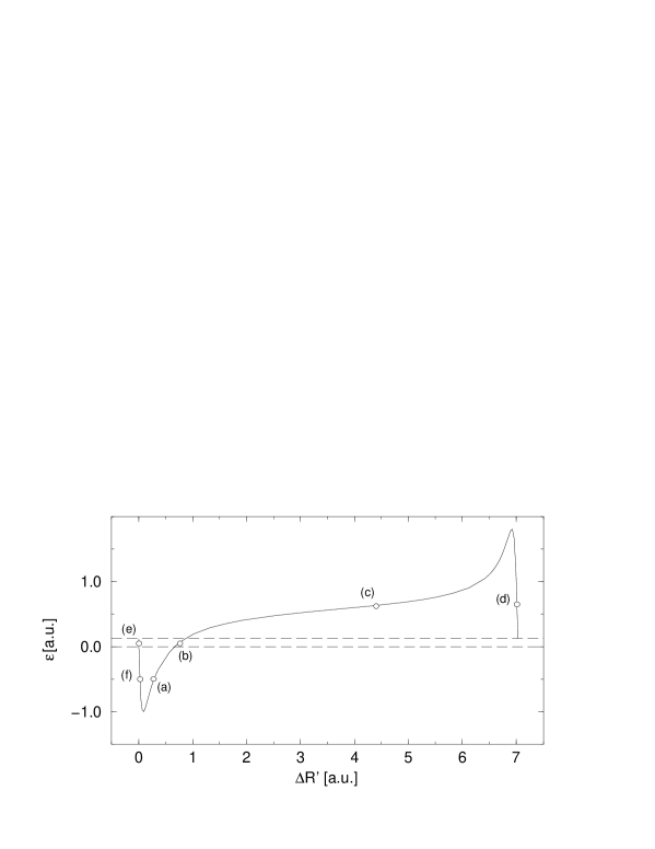
Figure 2: The deflection function at an energy of $E=0.125$ a.u. and for an initial state as described in the text. The energy interval enclosed by dashed lines marks ionizing initial conditions and separates the exchange region (${\epsilon}<0$) from the excitation region (${\epsilon}>E$), where ${\epsilon}$ is the energy of the projectile after the collision.

Figure 3: The deflection function at an energy of $E=2$ a.u. and for an initial state as described in the text. The dashed line separates ionizing initial conditions from excitation events.

2.2.2 The form of the collisional action

The collisional action $\Phi_{j}$ along the trajectory $j$ in (6) has some special properties which result from the form of the S-matrix (4). The asymptotically constant states are represented by a constant action $J$ or quantum number $n$ and a constant momentum $P$ for bound and free degrees of freedom respectively. Hence, in the asymptotic integrable situation with $\dot{n}=\dot{P}=0$ before and after the collision no action $\Phi_{j}$ is accumulated and the collisional action has a well defined value irrespectively of the actual propagation time in the asymptotic regions. This is evident from (8) which is, however, not suitable for a numerical realization of the collision. The scattering process is much easier followed in coordinate space, and more specifically for our collinear case, in radial coordinates. In the following, we will describe how to extract the action according to (8) from such a calculation in radial coordinates (position $r$ and momentum $p$ for the target electron, $R$ and $P$ for the projectile electron). The discussion refers to excitation processes to keep the notation simple but the result (13) holds also for the other cases. The collisional action $\Phi$ can be expressed through the action in coordinate space $\tilde{\Phi}$ by [3]

$$\Phi(P,n;P^{\prime},n^{\prime})=\tilde{\Phi}(P,r;P^{\prime},r^{\prime})+F_{2}(r^{\prime},n^{\prime})-F_{2}(r,n),$$ (10)

where

$$\tilde{\Phi}(P,r;P^{\prime},r^{\prime})=\lim_{t\to\,\infty\atop t^{\prime}\to-\infty}\,\int\limits_{t^{\prime}}^{t}\,d\tau\left[-R\dot{P}+p\dot{r}\right]$$ (11)

is the action in coordinate space and $F_{2}$ is the generator for the classical canonical transformation from the phase space variables $(r,p)$ to $(q,n)$ given by

$$F_{2}(r,n)={\rm{sgn}}(p)\,\int\limits_{r_{i}}^{r}\left(2m\left[\epsilon\left(n\right)-v\left(x\right)\right]\right)^{\frac{1}{2}}\,dx\,.$$ (12)

Here, $r_{i}$ denotes an inner turning point of an electron with energy $\epsilon(n)$ in the potential $v(x)$. Clearly, $F_{2}$ will not contribute if the trajectory starts end ends at a turning point of the bound electron. Partial integration of (11) transforms to momentum space and yields a simple expression for the collisional action in terms of spatial coordinates:

$$\Phi(P,n;P^{\prime},n^{\prime})=\lim_{t_{i}\to\,\infty\atop t_{i}^{\prime}\to-\infty}\,-\int\limits_{t_{i}^{\prime}}^{t_{i}}\,d\tau\left[R\dot{P}+r\dot{p}\right]\,.$$ (13)

Note, that $t_{i}^{\prime}$ and $t_{i}$ refer to times where the bound electron is at an inner turning point and the generator $F_{2}$ vanishes. Phases determined according to (13) may still differ for the same path depending on its time of termination. However, the difference can only amount to integer multiples of the (quantized !) action

$$J=\oint p\,dr=2\pi\left(n+\frac{1}{2}\right)$$ (14)

of the bound electron with $\epsilon<0$. Multiples of $2\pi$ for each revolution do not change the value of the S-matrix and the factor $\frac{2\pi}{2}$ is compensated by the Maslov index. In the case of an ionizing trajectory the action must be corrected for the logarithmic phase accumulated in Coulomb potentials [18].

Summarizing this analysis, we fix the (in principle arbitrary) starting point of the trajectory to be an inner turning point ($r_{i}^{\prime}|p^{\prime}=0,\dot{p}^{\prime}>0$) which completes the initial condition for the propagation of trajectories described in section 2.2.1. In order to obtain the correct collisional action (8) in the form (13) we also terminate a trajectory at an inner turning point $r_{i}$ after the collision such that $\Phi$ is a continuous function of the initial position $R^{\prime}$. Although this is not necessary for the primitive semiclassical scattering probability which is only sensitive to phase differences up to multiples of $J$ as mentioned above, the absolute phase difference is needed for a uniformized semiclassical expression to be discussed later.

2.3 Maslov indices

2.3.1 Numerical procedure

In position space the determination of the Maslov index is rather simple for an ordinary Hamiltonian with kinetic energy as in (2). According to Morse’s theorem the Maslov index is equal to the number of conjugate points along the trajectory. A conjugate point in coordinate space is defined by ($f$ degrees of freedom, $(q_{i},p_{i})$ a pair of conjugate variables)

$$det\left(M_{qp}\right)=det\left(\frac{\partial\left(q_{1},\ldots,q_{f}\right)}{\partial\left(p_{1}^{\prime},\ldots,p_{f}^{\prime}\right)}\right)=0.$$ (15)

The matrix $M_{qp}$ is the upper right part of the stability or monodromy matrix which is defined by

$${\delta\vec{q}(t)\choose\delta\vec{p}(t)}\equiv M(t)\,{\delta\vec{q}(0)\choose\delta\vec{p}(0)}\,.$$ (16)

In general, the Maslov index $\nu_{j}$ in (6) must be computed in the same representation as the action. In our case this is the momentum representation in (13). However, the Maslov index in momentum space is not simply the number of conjugate points in momentum space where $det\left(M_{pq}\right)=0$. Morse’s theorem relies on the fact that in position space the mass tensor $B_{ij}=\partial^{2}H/\partial p_{i}\partial p_{j}$ is positive definite. This is not necessarily true for $D_{ij}=\partial^{2}H/\partial q_{i}\partial q_{j}$ which is the equivalent of the mass tensor in momentum space. How to obtain the correct Maslov index from the number of zeros of $\det\left(M_{pq}\right)=0$ is described in [20], a review about the Maslov index and its geometrical interpretation is given in [21].

2.3.2 Phenomenological approach for two degrees of freedom

For two degrees of freedom, one can extract the scattering probability directly from the deflection function without having to compute the stability matrix and its determinant explicitly [8]. In view of this simplification it would be desirable to determine the Maslov indices also directly from the deflection function avoiding the complicated procedure described in the previous section. This is indeed possible since one needs only the correct difference of Maslov indices for a semiclassical scattering amplitude.

A little thought reveals that trajectories starting from branches in the deflection function of figure 2 separated by an extremum differ by one conjugate point. This implies that their respective Maslov indices differ by $\Delta\nu=1$. For this reason it is convenient to divide the deflection function in different branches, separated by an extremum. Trajectories of one branch have the same Maslov index. Since there are two extrema we need only two Maslov indices, $\nu_{1}=1$ and $\nu_{2}=2$. The relevance of just two values of Maslov indices $(1,2)$ can be traced to the fact that almost all conjugate points are trivial in the sense that they belong to turning points of bound two-body motion.

We can assign the larger index $\nu_{2}=2$ to the trajectories which have passed one more conjugate point than the others. As it is almost evident from their topology, these are the trajectories with $d{\epsilon}/dR^{\prime}>0$ shown in the upper row of figure 1. (They also have a larger collisional action $\Phi_{j}$). The two non-trivial conjugate points for these trajectories compared to the single conjugate point for orbits with initial conditions corresponding to $d{\epsilon}/dR^{\prime}<0$ can be understood looking at the ionizing trajectories (b) and (e) of each branch in figure 1. Trajectories from both branches have in common the turning point for the projectile electron ($P=0$). For trajectories of the lower row all other turning points belong to complete two-body revolutions of a bound electron and may be regarded as trivial conjugate points. However, for the trajectories from the upper row there is one additional turning point (see, e.g., figure 1(b)) which cannot be absorbed by a complete two-body revolution. It is the source for the additional Maslov phase.

We finally remark that $d\epsilon/dR^{\prime}>0$ is equivalent to $dn/d\bar{q}<0$ of [25] leading to the same result as our considerations illustrated above.

3 Semiclassical scattering probabilities

Taking into account the Pauli principle for the indistinguishable electrons leads to different excitation probabilities for singlet and triplet,

$$P^{+}_{\epsilon}(E) = \left|\,S_{\epsilon,\epsilon^{\prime}}(E)+S_{E-\epsilon,\epsilon^{\prime}}(E)\,\right|^{2}$$

$$P^{-}_{\epsilon}(E) = \left|\,S_{\epsilon,\epsilon^{\prime}}(E)-S_{E-\epsilon,\epsilon^{\prime}}(E)\,\right|^{2}\,,$$ (17)

where the probabilities are symmetrized a posteriori (see [24]). Here, $S_{\epsilon,\epsilon^{\prime}}$ denotes the S-matrix for the excitation branch, calculated according to (6), while $S_{E-\epsilon,\epsilon^{\prime}}$ represents the exchange processes, at a fixed energy $\epsilon<0$, respectively.

Ionization probabilities are obtained by integrating the differential probabilities over the relevant energy range which is due to the symmetrization (17) reduced to $E/2$:

$$P^{\pm}_{ion}(E)=\int\limits_{0}^{E/2}P^{\pm}_{\epsilon}(E)\,d\epsilon\,.$$ (18)

3.1 Ionization and excitation for singlet and triplet symmetry

We begin with the ionization probabilities since they illustrate most clearly the effect of the vanishing exchange branch for higher energies as illustrated in figure 3. The semiclassical result for the Langer Hamiltonian (2) shows the effect of the vanishing exchange branch in the deflection function figure 3 which leads to merging $P^{\pm}$ probabilities at a finite energy $E$, in clear discrepancy to the quantum result, see figure 4. Moreover, the extrema in the deflection function lead to the sharp structures below $E=1$ a.u.. The same is true for the excitation probabilities where a discontinuity appears below $E=1$ a.u. (figure 5). Note also that due to the violated unitarity in the semiclassical approximation probabilities can become larger than unity, as it is the case for the $n=1$ channel.

Figure 4: Ionization probabilities for singlet and triplet according to (18) with the Hamiltonian (2) (solid line) compared to quantum mechanical calculations (dotted line).

Figure 5: Semiclassical excitation probabilities ($n=1,2,3$) according to (17) for singlet (part a) and triplet (part b) in the LSA (solid line) compared to quantum mechanical calculations (dotted line).

Singlet and triplet excitation probabilities represent the most differential scattering information for the present collisional system. Hence, the strongest deviations of the semiclassical results from the quantum values can be expected. Most experiments do not resolve the spin states and measure a spin-averaged signal. In our model this can be simulated by averaging the singlet and triplet probabilities to

$$P_{\epsilon}(E)=\frac{1}{2}(P^{+}_{\epsilon}(E)+P^{-}_{\epsilon}(E)).$$ (19)

The averaged semiclassical probabilities may also be compared to the classical result which is simply given by

$$P^{CL}_{\epsilon}(E)=\sum_{j}({\cal P}^{(j)}_{\epsilon,\epsilon^{\prime}}(E)+{\cal P}^{(j)}_{\epsilon,E-\epsilon^{\prime}}(E))$$ (20)

with ${\cal P}^{(j)}_{\epsilon,\epsilon^{\prime}}(E)$ from (7).

Figure 6 shows averaged ionization probabilities. They are very similar to each other, and indeed, the classical result is not much worse than the semiclassical result.

Figure 6: Spin averaged quantum results for ionization (dotted line) compared to averaged semiclassical probabilities (solid line) from (19) and classical probabilities (dashed line) from (20).

In figure 7 we present the averaged excitation probabilities. Again, on can see the discontinuity resulting from the extrema in the deflection function. As for ionization, the spin averaged semiclassical probabilities (figure 7b) are rather similar to the classical ones (figure 7a), in particular the discontinuity is of the same magnitude as in the classical case and considerably more localized in energy than in the non-averaged quantities of figure 5.

Figure 7: Spin averaged quantum results (dotted line) for excitation ($n=1,2,3$) compared to classical probabilities (solid line, part a) from (20) and averaged semiclassical probabilities (solid line, part b) from (19).

Clearly, the discontinuities are an artefact of the semiclassical approximation. More precisely, they are a result of the finite depth of the two-body potential in the Langer corrected Hamiltonian (2). Around the extrema of the deflection function the condition of isolated stationary points, necessary to apply the stationary phase approximation which leads to (6), is not fulfilled. Rather, one has to formulate a uniform approximation which can handle the coalescence of two stationary phase points.

4 Uniformized scattering probabilities

We follow an approach by Chester et. al. [23]. The explicit expression for the uniform S-matrix goes back to Connor and Marcus [22] who obtained for two coalescing trajectories $1$ and $2$

$$S_{n,n^{\prime}}(E)={\rm Bi}^{+}\left(-z\right)\,\sqrt{{\cal P}_{n,n^{\prime}}^{(1)}(E)}\,e^{i\Phi_{1}+i\frac{\pi}{4}}\,+\,{\rm Bi}^{-}\left(-z\right)\,\sqrt{{\cal P}_{n,n^{\prime}}^{(2)}(E)}\,e^{i\Phi_{2}-i\frac{\pi}{4}}$$ (21)

where

$${\rm Bi}^{\pm}\left(-z\right)=\sqrt{\pi}\left[z^{\frac{1}{4}}{\rm Ai}\left(-z\right)\mp iz^{-\frac{1}{4}}{\rm Ai}^{\prime}\left(-z\right)\right]\,e^{\pm i\left(\frac{2}{3}z^{\frac{3}{2}}-\frac{\pi}{4}\right)}$$ (22)

The argument $z=\left[\frac{3}{4}\left(\Phi_{2}-\Phi_{1}\right)\right]^{\frac{2}{3}}$ of the Airy function Ai(z) contains the absolute phase difference. We assume that $\Phi_{2}>\Phi_{1}$ which implies for the difference of the Maslov indices that $\nu_{2}-\nu_{1}=1$ (compare (6) with (21) and (23)). Since the absolute phase difference enters (21) it is important to ensure that the action is a continuous function of $R^{\prime}$ avoiding jumps of multiples of $2\pi$, as already mentioned in section 2.2.2. For large phase differences (6) is recovered since

$$\lim_{z\to\infty}{\rm Bi}^{\pm}\left(-z\right)=1\,.$$ (23)

Our uniformized S-matrix has been calculated by applying (21) to the two branches for exchange and excitation separately and adding or subtracting the results according to a singlet or triplet probability. In the corresponding probabilities of figure 8 the discontinuities of the non-uniform results are indeed smoothed in comparison with figure 5. However, the overall agreement with the quantum probabilities is worse than in the non-uniform approximation. A possible explanation could lie in the construction of the uniform approximation. It works with an integral representation of the S-matrix, where the oscillating phase (the action) is mapped onto a cubic polynomial. As a result, the uniformization works best, if the deflection function can be described as a quadratic function around the extremum. Looking at figure 2 one sees that this is true only in a very small neighborhood of the extrema because the deflection function is strongly asymmetric around these points. We also applied a uniform approximation derived by Miller [4] which gave almost identical results.

Figure 8: Uniformized semiclassical excitation probabilities ($n=1,2,3$) according to (21) (solid line) for singlet (part a) and triplet (part b) compared to quantum mechanical calculations (dotted line).

Finally, for the sake of completeness, the spin averaged uniform probabilities are shown in figure 9. As can be seen, the discontinuities have vanished almost completely. However, the general agreement with quantum mechanics is worse than for the standard semiclassical calculations, similarly as for the symmetrized probabilities.

Figure 9: Spin averaged uniformized excitation probabilities ($n=1,2,3$, solid line) compared to quantum results (dotted line).

5 Conclusion

In this paper we have described inelastic Coulomb scattering with a semiclassical S-matrix. To handle the problem for this explorative study we have restricted the phase space to the collinear arrangement of the two electrons reducing the degrees of freedom to one radial coordinate for each electron. In appreciation of the spherical geometry we have applied the so called Langer correction to obtain the correct angular momentum quantization. Thereby, a lower bound to the two-body potential is introduced which generates a generic situation for bound state dynamics since the (singular) Coulomb potential is replaced by a potential bounded from below. The finite depth of the two-body potential leads to singularities in the semiclassical scattering matrix (rainbow effect) which call for a uniformization.

Hence, we have carried out and compared among each other classical (where applicable), semiclassical, and uniformized semiclassical calculations for the singlet, triplet and spin-averaged ionization and excitation probabilities. Two general trends may be summarized: Firstly, the simple semiclassical probabilities are overall in better agreement with the quantum results for the singlet/triplet observables than the uniformized results. The latter are only superior close to the singularities. Secondly, for the (experimentally most relevant) spin-averaged probabilities the classical (non-symmetrizable) result is almost as good as the semiclassical one compared to the exact quantum probability. This holds for excitation as well as for ionization. Hence, we conclude from our explorative study that a full semiclassical treatment for spin-averaged observables is probably not worthwhile since it does not produce better results than the much simpler classical approach. Clearly, this conclusion has to be taken with some caution since we have only explored a collinear, low dimensional phase space.

References

References

- [1] Ford K W and Wheeler J A 1959 Ann. Phys. 7 259
- [2] Pechukas P 1969 Phys. Rev. 181 166
- [3] Miller W H 1970 J. Chem. Phys. 53 1949
-
[4]
Miller W H 1970 J. Chem. Phys. 53 3578
Miller W H 1970 Chem. Phys. Lett. 7 431 -
[5]
Miller W H 1974 Adv. Chem. Phys. 25 69
Miller W H 1975 Adv. Chem. Phys. 30 77 - [6] Balian R and Bloch C 1974 Ann. Phys. 85 514
- [7] Rost J M and Heller E J 1994 J. Phys. B: At. Mol. Opt. Phys. 27 1387
- [8] Rost J M 1994 Phys. Rev. Lett. 72 1998
- [9] Rost J M 1995 J. Phys. B: At. Mol. Opt. Phys. 28 3003
- [10] Rost J M and Wintgen D 1996 Europhys. Lett. 35 19
- [11] Gu Y and Yuan J M 1993 Phys. Rev. A 47 R2442
-
[12]
Ezra G S, Richter K, Tanner G and Wintgen D 1991 J. Phys. B: At. Mol. Opt. Phys. 24 L413
Wintgen D, Richter K and Tanner G 1992 CHAOS 2 19
Tanner G and Wintgen D 1995 Phys. Rev. Lett. 75 2928 - [13] Wannier G H 1953 Phys. Rev. 90 817
- [14] Rost J M 1998 Phys. Rep. 297 291
- [15] Handke G, Draeger M, Ihra W and Friedrich H 1993 Phys. Rev. A 48 3699
- [16] Friedrich H, Ihra W and Meerwald P 1999 Aust. J. Phys. 52 323
- [17] Langer R 1937 Phys. Rev. 51 669
- [18] Child M S 1974 Molecular Collision Theory (London: Academic Press)
- [19] Yoshida H 1990 Phys. Lett. A 150 262
- [20] Levit S, Möhring K, Smilansky U and Dreyfus T 1978 Ann. Phys. 114 223
- [21] Littlejohn R G 1992 J. Stat. Phys. 68 7
- [22] Connor J N L and Marcus R A 1971 J. Chem. Phys. 55 5636
- [23] Chester C, Friedman B and Ursell F 1957 Proc. Camb. phil. Soc. 53 555
- [24] Joachain C J 1975 Quantum Collision Theory (Amsterdam: North Holland)
- [25] Marcus R 1972 Chem. Phys. 57 4903