Capillary-gravity wave transport over spatially random drift

Abstract

We derive transport equations for the propagation of water wave action in the presence of a static, spatially random surface drift. Using the Wigner distribution ${\bf W}({\bf x},{\bf k},t)$ to represent the envelope of the wave amplitude at position ${\bf x}$ contained in waves with wavevector ${\bf k}$, we describe surface wave transport over static flows consisting of two length scales; one varying smoothly on the wavelength scale, the other varying on a scale comparable to the wavelength. The spatially rapidly varying but weak surface flows augment the characteristic equations with scattering terms that are explicit functions of the correlations of the random surface currents. These scattering terms depend parametrically on the magnitudes and directions of the smoothly varying drift and are shown to give rise to a Doppler coupled scattering mechanism. The Doppler interaction in the presence of slowly varying drift modifies the scattering processes and provides a mechanism for coupling long wavelengths with short wavelengths. Conservation of wave action (CWA), typically derived for slowly varying drift, is extended to systems with rapidly varying flow. At yet larger propagation distances, we derive from the transport equations, an equation for wave energy diffusion. The associated diffusion constant is also expressed in terms of the surface flow correlations. Our results provide a formal set of equations to analyse transport of surface wave action, intensity, energy, and wave scattering as a function of the slowly varying drifts and the correlation functions of the random, highly oscillatory surface flows.

1 Introduction

Water wave dynamics are altered by interactions with spatially varying surface flows. The surface flows modify the free surface boundary conditions that determine the dispersion for propagating water waves. The effect of smoothly varying (compared to the wavelength) currents have been analysed using ray theory ([Peregrine (1976), Jonsson (1990)]) and the principle of conservation of wave action (CWA) (cf. [Longuet-Higgins & Stewart (1961), Mei (1979), White (1999), Whitham (1974)] and references within). These studies have largely focussed on long ocean gravity waves propagating over even larger scale spatially varying drifts. Water waves can also scatter from regions of underlying vorticity regions smaller than the wavelength [Fabrikant & Raevsky (1994)] and [Cerda & Lund (1993)]. Boundary conditions that vary on capillary length scales, as well as wave interactions with structures comparable to or smaller than the wavelength can also lead to wave scattering ([Chou, Lucas & Stone (1995), Gou, Messiter & Schultz (1993)]), attenuation ([Chou & Nelson (1994), Lee et al. (1993)]), and Bragg reflections ([Chou (1998), Naciri & Mei (1988)]). Nonetheless, water wave propagation over random static underlying currents that vary on both large and small length scales, and their interactions, have received relatively less attention.

In this paper, we will only consider static irrotational currents, but derive the transport equations for surface waves in the presence of underlying flows that vary on both long and short (on the order of the wavelength) length scales. Rather than computing wave scattering from specific static flow configurations ([Gerber (1993), Trulson & Mei (1993), Fabrikant & Raevsky (1994)]), we take a statistical approach by considering ensemble averages over realisations of the static randomness. Different statistical approaches have been applied to wave propagation over a random depth ([Elter & Molyneux (1972)]), third sound localization in superfluid Helium films ([Kleinert (1990)]), and wave diffusion in the presence of turbulent flows ([Howe (1973), Rayevskiy (1983), Fannjiang & Ryzhik (1999)]).

In the next section we derive the linearised capillary-gravity wave equations to lowest order in the irrotational surface flow. The fluid mechanical boundary conditions are reduced to two partial differential equations that couple the surface height to velocity potential at the free surface. We treat only the “high frequency” limit ([Ryzhik, Papanicolaou, & Keller (1996)]) where wavelengths are much smaller than wave propagation distances under consideration. In Section 3, we introduce the Wigner distribution ${\bf W}({\bf x},{\bf k},t)$ which represents the wave energy density and allows us to treat surface currents that vary simultaneously on two separated length scales. The dynamical equations developed in section 2 are then written in terms of an evolution equation for ${\bf W}$. Upon expanding ${\bf W}$ in powers of wavelength/propagation distance, we obtain transport equations.

In Section 4, we present our main mathematical result, equation (35), an equation describing the transport of surface wave action. Appendix A gives details of some of the derivation. The transport equation includes advection by the slowly varying drift, plus scattering terms that are functions of the correlations of the rapidly varying drift, representing water wave scattering. Upon simultaneously treating both smoothly varying and rapidly varying flows using a two-scale expansion, we find that scattering from rapidly varying flows depends parametrically on the smoothly varying flows. In the Results and Discussion, we discuss the regimes of validity, consider specific forms for the correlation functions, and detail the conditions for doppler coupling. CWA is extended to include rapidly varying drift provided that the correlations of the drift satisfy certain constraints. We also physically motivate the reason for considering two scales for the underlying drift. In the limit of still larger propagation distances, after multiple wave scattering, wave propagation leaves the transport regime and becomes diffusive ([Sheng (1995)]). A diffusion equation for water wave energy is also given, with an outline of its derivation given in Appendix B.

2 Surface wave equations

Assume an underlying flow ${\bf V}({\bf x},z)\equiv(U_{1}({\bf x},z),U_{2}({\bf x},z),U_{z}({\bf x},z))\equiv({\bf U}({\bf x},z),U_{z}({\bf x},z))$, where the 1,2 components denote the two-dimensional in-plane directions. This static flow may be generated by external, time independent sources such as wind or internal flows beneath the water surface. The surface deformation due to ${\bf V}({\bf x},z)$ is denoted $\bar{\eta}({\bf x})$ where ${\bf x}\equiv(x,y)$ is the two-dimensional in-plane position vector. An additional variation in height due to the velocity ${\bf v}({\bf x},z)$ associated with surface waves is denoted $\eta({\bf x},t)$. When all flows are irrotational, we can define their associated velocity potentials ${\bf V}({\bf x},z)\equiv(\nabla_{{\bf x}}+\hat{{\bf z}}\partial_{z})\Phi({\bf x},z)$ and ${\bf v}({\bf x},z,t)\equiv(\nabla_{{\bf x}}+\hat{{\bf z}}\partial_{z})\varphi({\bf x},z,t)$. Incompressibility requires

$$\Delta\varphi({\bf x},z,t)+\partial_{z}^{2}\varphi({\bf x},z,t)=\Delta\Phi({\bf x},z)+\partial_{z}^{2}\Phi({\bf x},z)=0,$$ (1)

where $\Delta=\nabla_{{\bf x}}^{2}$ is the two-dimensional Laplacian. The kinematic condition ([Whitham (1974)]) applied at $z=\bar{\eta}({\bf x})+\eta({\bf x},t)\equiv\zeta({\bf x},t)$ is

$$\partial_{t}\eta({\bf x},t)+{\bf U}({\bf x},\zeta)\cdot\nabla_{{\bf x}}\zeta({\bf x},t)=U_{z}({\bf x},z=\zeta)+\partial_{z}\varphi({\bf x},z=\zeta,t).$$ (2)

Upon expanding (2) to linear order in $\eta$ and $\varphi$ about the static free surface, the right hand side becomes

$$U_{z}({\bf x},\zeta)+\partial_{z}\varphi({\bf x},\zeta,t)=U_{z}({\bf x},\bar{\eta})+\eta({\bf x},t)\partial_{z}U_{z}({\bf x},\bar{\eta})+\partial_{z}\varphi({\bf x},\bar{\eta},t)+O(\eta^{2}).$$ (3)

At the static surface $\bar{\eta}$, ${\bf U}({\bf x},\bar{\eta})\cdot\nabla_{{\bf x}}\bar{\eta}({\bf x})=U_{z}({\bf x},\bar{\eta})$. Now assume that the underlying flow is weak enough such that $U_{z}({\bf x},z\approx 0)$ and $\bar{\eta}$ are both small. A rigid surface approximation is appropriate for small Froude numbers $U^{2}/c^{2}_{\phi}\sim|\nabla_{{\bf x}}\bar{\eta}|^{2}\sim U_{z}({\bf x},0)/|{\bf U}({\bf x},0)|\ll 1$ ($c_{\phi}$ is the surface wave phase velocity) when the free surface boundary conditions can be approximately evaluated at $z=0$ ([Fabrikant & Raevsky (1994)]). Although we have assumed $U_{z}({\bf x},z\approx 0)=\partial_{z}\Phi({\bf x},z\approx 0)\approx 0$ and a vanishing static surface deformation $\bar{\eta}({\bf x})\approx 0$, $\nabla_{{\bf x}}\cdot{\bf U}({\bf x},0)=-\partial_{z}U_{z}({\bf x},0)\neq 0$.

Combining the above approximations with the dynamic boundary conditions (derived from balance of normal surface stresses at $z=0$ ([Whitham (1974)])), we have the pair of coupled equations

$$\begin{array}[]{l}\displaystyle\partial_{t}\eta({\bf x},t)+\nabla_{{\bf x}}\cdot\left({\bf U}({\bf x},z=0)\eta({\bf x},t)\right)=\lim_{z\rightarrow 0^{-}}\partial_{z}\varphi({\bf x},z,t)\\[13.0pt] \displaystyle\lim_{z\rightarrow 0^{-}}\left[\rho\partial_{t}\varphi({\bf x},z,t)+\rho{\bf U}({\bf x},z)\cdot\nabla_{{\bf x}}\varphi({\bf x},z,t)\right]=\sigma\Delta\eta({\bf x},t)-\rho g\eta({\bf x},t)\end{array}$$ (4)

where $\sigma$ and $g$ are the air-water surface tension and gravitational acceleration, respectively. Although it is straightforward to expand to higher orders in $\bar{\eta}({\bf x})$ and $\eta({\bf x},t)$, or to include underlying vorticity, we will limit our study to equations (4) in order to make the development of the transport equations more transparent.

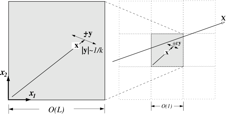
Figure 1: The relevant scales in water wave transport. Initially, the system size, observation point, and length scale of the slowly varying drift is $O(L)$, with surface wave wavelength and scale of the random surface current of $O(1)$. Upon rescaling, the system size becomes $O(1)$, while the wavelength and random flow variations are $O(\varepsilon)$.

The typical system size, or distance of wave propagation shown in Fig. 1 is of $O(L)$ with $L\gg 1$. Wavelengths however, are of $O(1)$. To implement our high frequency ([Ryzhik, Papanicolaou, & Keller (1996)]) asymptotic analyses, we rescale the system such that all distances are measured in units of $L\equiv\varepsilon^{-1}$. We eventually take the limit $\varepsilon\rightarrow 0$ as an approximation for small, finite $\varepsilon$. Surface velocities, potentials, and height displacements are now functions of the new variables ${\bf x}\rightarrow{\bf x}/\varepsilon,z\rightarrow z/\varepsilon$ and $t\rightarrow t/\varepsilon$. We shall further nondimensionalise all distances in terms of the capillary length $\ell_{c}=\sqrt{\sigma/g\rho}$. Time, velocity potentials, and velocities are dimensionalised in units of $\sqrt{\ell_{c}/g},\sqrt{g\ell_{c}^{3}}$, and $\sqrt{g\ell_{c}}$ respectively, e.g. for water, $U=1$ corresponds to a surface drift velocity of $\sim 16.3$cm/s.

Since $U_{z}({\bf x},z\approx 0)\approx 0$, we define the flow at the surface by

$${\bf U}({\bf x},z=0)\equiv{\bf U}({\bf x})+\sqrt{\varepsilon}\delta{\bf U}({\bf x}/\varepsilon).$$ (5)

In these rescaled coordinates, ${\bf U}({\bf x})$ denotes surface flows varying on length scales of $O(1)$ much greater than a typical wavelength, while $\delta{\bf U}({\bf x}/\varepsilon)$ varies over lengths of $O(\varepsilon)$ comparable to a typical wavelength. The amplitude of the slowly varying flow ${\bf U}({\bf x})$ is $O(\varepsilon^{0})$, while that of the rapidly varying flow $\delta{\bf U}({\bf x}/\varepsilon)$, is assumed to be of $O(\sqrt{\varepsilon})$. A more detailed discussion of the physical motivation for considering the $\sqrt{\varepsilon}$ scaling is deferred to the Results and Discussion. After rescaling, the boundary conditions (4) evaluated at $z=0$ become

$$\begin{array}[]{l}\displaystyle\partial_{t}\eta({\bf x},t)+\nabla_{{\bf x}}\cdot\left[\left({\bf U}({\bf x})+\sqrt{\varepsilon}\delta{\bf U}({\bf x}/\varepsilon)\right)\eta({\bf x})\right]=\lim_{z\rightarrow 0^{-}}\partial_{z}\varphi({\bf x},0)\\[13.0pt] \displaystyle\partial_{t}\varphi({\bf x},t)+{\bf U}({\bf x})\cdot\nabla_{{\bf x}}\varphi({\bf x},t)+\sqrt{\varepsilon}\delta{\bf U}({\bf x}/\varepsilon)\cdot\nabla_{{\bf x}}\varphi({\bf x},t)=\varepsilon\Delta\eta({\bf x},t)-\varepsilon^{-1}\eta({\bf x},t).\end{array}$$ (6)

Although drift that varies slowly along one wavelength can be treated with characteristics and WKB theory, random flows varying on the wavelength scale require a statistical approach. Without loss of generality, we choose $\delta{\bf U}$ to have zero mean and an isotropic two-point correlation function $\langle\delta U_{i}({\bf x})\delta U_{j}({\bf x}^{\prime})\rangle\equiv R_{ij}(|{\bf x}-{\bf x}^{\prime}|)$, where $(i,j)=(1,2)$ and $\langle\ldots\rangle$ denotes an ensemble average over realisations of $\delta{\bf U}({\bf x})$.

We now define the spatial Fourier decompositions for the dynamical wave variables

$$\begin{array}[]{ll}\displaystyle\varphi({\bf x},-h\leq z\leq\zeta,t)=\int_{{\bf q}}\,\varphi({\bf q},t)e^{-i{\bf q}\cdot{\bf x}}{\cosh q(h+z)\over\cosh qh},&\displaystyle\eta({\bf x},t)=\int_{{\bf q}}\,\eta({\bf q},t)e^{-i{\bf q}\cdot{\bf x}},\end{array}$$ (7)

the static surface flows

$$\begin{array}[]{ll}\displaystyle{\bf U}({\bf x})=\int_{{\bf q}}{\bf U}({\bf q})e^{-i{\bf q}\cdot{\bf x}},&\displaystyle\delta{\bf U}\left({{\bf x}\over\varepsilon}\right)=\int_{{\bf q}}\delta{\bf U}({\bf q})e^{-i{\bf q}\cdot{\bf x}/\varepsilon},\end{array}$$ (8)

and the correlations

$$R_{ij}({\bf x})=\int_{{\bf q}}R_{ij}({\bf q})e^{-i{\bf q}\cdot{\bf x}},$$ (9)

where ${\bf q}=(q_{1},q_{2})$ is an in-plane two dimensional wavevector, $q\equiv|{\bf q}|=\sqrt{q_{1}^{2}+q_{2}^{2}}$, and $\int_{{\bf q}}\equiv(2\pi)^{-2}\int dq_{1}dq_{2}$. The Fourier integrals for $\eta$ exclude ${\bf q}=0$ due to the incompressibility constraint $\int_{\bf x}\eta({\bf x},t)=0$, while the ${\bf q}=0$ mode for $\varphi$ gives an irrelevant constant shift to the velocity potential. Note that $\varphi$ in (7) manifestly satisfies (1). Substituting (8) into the boundary conditions (4), we obtain,

$$\begin{array}[]{l}\displaystyle\partial_{t}\eta({\bf k},t)-i\int_{{\bf q}}\eta({\bf k}-{\bf q}){\bf U}({\bf q})\cdot{\bf k}-i\sqrt{\varepsilon}\int_{{\bf q}}\eta({\bf k}-{\bf q}/\varepsilon)\delta{\bf U}({\bf q})\cdot{\bf k}=\varphi({\bf k},t)\,k\tanh\varepsilon kh\\[13.0pt] \displaystyle\partial_{t}\varphi({\bf k},t)-i\int_{{\bf q}}{\bf U}({\bf q})\cdot\left({\bf k}-{\bf q}\right)\varphi({\bf k}-{\bf q})-i\sqrt{\varepsilon}\int_{{\bf q}}\delta{\bf U}({\bf q})\cdot\left({\bf k}-{\bf q}/\varepsilon\right)\varphi({\bf k}-{\bf q}/\varepsilon)\\[13.0pt] \hskip 216.81pt=-(\varepsilon k^{2}+\varepsilon^{-1})\eta({\bf k}).\end{array}$$ (10)

where the $\delta{\bf U}({\bf q})$ are correlated according to

$$\langle\delta U_{i}({\bf p})\delta U_{j}({\bf q})\rangle=R_{ij}(|{\bf p}|)\delta({\bf p}+{\bf q}).$$ (11)

Since the correlation $R_{ij}({\bf x})$ is symmetric in $i\leftrightarrow j$, and depends only upon the magnitude $|{\bf x}|$, $R_{ij}(|{\bf p}-{\bf q}|)$ is real.

In the case where $\delta{\bf U}=0$ and ${\bf U}({\bf x})\equiv{\bf U}_{0}$ is strictly uniform, equations (10) can be simplified by assuming a $e^{-i\omega t}$ dependence for all dynamical variables. Uniform drift yields the familiar capillary-gravity wave dispersion relation

$$\omega({\bf k})=\sqrt{(k^{3}+k)\tanh kh}+{\bf U}_{0}\cdot{\bf k}\equiv\Omega({\bf k})+{\bf U}_{0}\cdot{\bf k}.$$ (12)

However, for what follows, we wish to derive transport equations for surface waves (action, energy, intensity) in the presence of a spatially varying drift containing two length scales: ${\bf U}={\bf U}({\bf x})+\sqrt{\varepsilon}\delta{\bf U}({\bf x}/\varepsilon)$.

3 The Wigner distribution and asymptotic analyses

The intensity of the dynamical wave variables can be represented by the product of two Green functions evaluated at positions ${\bf x}\pm\varepsilon{\bf y}/2$. The difference in their evaluation points, $\varepsilon{\bf y}$, resolves the waves of wavevector $|{\bf k}|\sim 2\pi/(\varepsilon y)$. [Elter & Molyneux (1972)] used this representation to study shallow water wave propagation over a random bottom. However, for the arbitrary depth surface wave problem, where the Green function is not simple, and where two length scales are treated, it is convenient to use the Fourier representation of the Wigner distribution ([Wigner (1932), Gérard et al. (1997), Ryzhik, Papanicolaou, & Keller (1996)]).

Define $\boldsymbol{\psi}=(\psi_{1},\psi_{2})\equiv(\eta({\bf x}),\varphi({\bf x},z=0))$ and the Wigner distribution:

$$W_{ij}({\bf x},{\bf k},t)\equiv(2\pi)^{-2}\int e^{i{\bf k}\cdot{\bf y}}\psi_{i}\left({\bf x}-{\varepsilon{\bf y}\over 2},t\right)\psi^{*}_{j}\left({\bf x}+{\varepsilon{\bf y}\over 2},t\right)d{\bf y}$$ (13)

where ${\bf x}$ is a central field point from which we consider two neighbouring points ${\bf x}\pm{\varepsilon{\bf y}\over 2}$, and their intervening wave field. Fourier transforming the ${\bf x}$ variable using the definition (7) we find,

$$W_{ij}({\bf p},{\bf k},t)=(2\pi\varepsilon)^{-2}\psi_{i}\left({{\bf p}\over 2}-{{\bf k}\over\varepsilon},t\right)\psi^{*}_{j}\left(-{{\bf p}\over 2}-{{\bf k}\over\varepsilon},t\right).$$ (14)

The total wave energy, comprising gravitational, kinetic, and surface tension contributions is

$$\begin{array}[]{rl}{\cal E}=&\displaystyle{1\over 2}\int_{\bf x}\left[|\nabla_{{\bf x}}\eta({\bf x})|^{2}+|\eta({\bf x})|^{2}\right]+{1\over 2}\int_{\bf x}\int_{-h}^{0}dz|{\bf U}({\bf x},z)+{\bf\hat{z}}U_{z}({\bf x},z)+{\bf v}({\bf x},z)|^{2}\\[13.0pt] &\displaystyle\hskip 56.9055pt-{1\over 2}\int_{\bf x}\int_{-h}^{0}dz|{\bf U}({\bf x},z)+{\bf\hat{z}}U_{z}({\bf x},z)|^{2}\\[13.0pt] &\displaystyle={1\over 2}\int_{{\bf k}}(k^{2}+1)|\eta({\bf k})|^{2}+k\tanh kh|\varphi({\bf k},z=0)|^{2}.\end{array}$$ (15)

The energy above has been expanded to an order in $\eta({\bf x},t)$ and $\varphi({\bf x},z,t)$ consistent with the approximations used to derive (4). In arriving at the last equality in (15), we have integrated by parts, used the Fourier decompositions (7) and imposed an impenetrable bottom condition at $z=-h$. The wave energy density carried by wavevector ${\bf k}$ is ([Gérard et al. (1997)])

$${\cal E}({\bf k},t)={1\over 2}\mbox{Tr}\left[{\bf A}({\bf k}){\bf W}({\bf k},t)\right],$$ (16)

where $A_{11}({\bf k})=k^{2}+1,A_{22}({\bf k})=k\tanh kh,A_{12}=A_{21}=0$. Thus, the Wigner distribution epitomises the local surface wave energy density.

In the presence of slowly varying drift, we identify ${\bf W}({\bf x},{\bf k},t)$ as the local Wigner distribution at position ${\bf x}$ representing waves of wavevector ${\bf k}$. The time evolution of its Fourier transform ${\bf W}({\bf p},{\bf k},t)$, can be derived by considering time evolution of the vector field $\boldsymbol{\psi}$ implied by the boundary conditions (4):

$$\begin{array}[]{ll}\displaystyle\dot{\psi}_{j}({\bf k},t)+iL_{j\ell}({\bf k})\psi_{\ell}({\bf k},t)=&\displaystyle i\int_{{\bf q}}{\bf U}({\bf q})\cdot({\bf k}-{\bf q}\delta_{j2})\psi_{j}({\bf k}-{\bf q},t)\\[13.0pt] &+i\sqrt{\varepsilon}\int_{{\bf q}}\delta{\bf U}({\bf q})\cdot({\bf k}-{\bf q}\delta_{j2}/\varepsilon)\psi_{j}({\bf k}-{\bf q}/\varepsilon,t),\end{array}$$ (17)

where the operator ${\bf L}({\bf k})$ is defined by

$${\bf L}({\bf k})=\left(\begin{array}[]{cc}0&i|{\bf k}|\tanh\varepsilon|{\bf k}|h\\[13.0pt] -i(\varepsilon k^{2}+\varepsilon^{-1})&0\end{array}\right).$$ (18)

We have redefined the physical wavenumber to be $k/\varepsilon$ so that $k\sim O(1)$. Upon using (17) and the definition (14), (see Appendix A)

$$\begin{array}[]{rl}\displaystyle\dot{W}_{ij}({\bf p},{\bf k},t)&\displaystyle=iW_{i\ell}({\bf p},{\bf k},t)L_{\ell j}^{\dagger}\left({{\bf k}\over\varepsilon}+{{\bf p}\over 2}\right)-iL_{i\ell}\left({{\bf k}\over\varepsilon}-{{\bf p}\over 2}\right)W_{\ell j}({\bf p},{\bf k},t)\\[13.0pt] &\displaystyle+i\int_{{\bf q}}{\bf U}({\bf q})\cdot\left(-{{\bf k}\over\varepsilon}+{{\bf p}\over 2}-{\bf q}\delta_{i2}\right)W_{ij}({\bf p}-{\bf q},{\bf k}+\varepsilon{\bf q}/2,t)\\[13.0pt] &\displaystyle-i\int_{{\bf q}}{\bf U}({\bf q})\cdot\left(-{{\bf k}\over\varepsilon}-{{\bf p}\over 2}+{\bf q}\delta_{j2}\right)W_{ij}({\bf p}-{\bf q},{\bf k}-\varepsilon{\bf q}/2,t)\\[13.0pt] &\displaystyle+i\sqrt{\varepsilon}\int_{{\bf q}}\delta{\bf U}({\bf q})\cdot\left(-{{\bf k}\over\varepsilon}+{{\bf p}\over 2}-{{\bf q}\over\varepsilon}\delta_{i2}\right)W_{ij}({\bf p}-{\bf q}/\varepsilon,{\bf k}+{\bf q}/2,t)\\[13.0pt] &\displaystyle-i\sqrt{\varepsilon}\int_{{\bf q}}\delta{\bf U}({\bf q})\cdot\left(-{{\bf k}\over\varepsilon}-{{\bf p}\over 2}+{{\bf q}\over\varepsilon}\delta_{j2}\right)W_{ij}({\bf p}-{\bf q}/\varepsilon,{\bf k}-{\bf q}/2,t),\end{array}$$ (19)

where only the index $\ell=1,2$ has been summed over. If we now assume that ${\bf W}({\bf x},{\bf k},t)$ can be expanded in functions that vary independently at the two relevant length scales, functions of the field ${\bf p}$ (dual to ${\bf x}$) can be replaced by functions of a slow variation in ${\bf p}$ and a fast oscillation $\boldsymbol{\xi}/\varepsilon$; ${\bf p}\rightarrow{\bf p}+\boldsymbol{\xi}/\varepsilon$.

This amounts to the Fourier equivalent of a two-scale expansion in which ${\bf x}$ is replaced by ${\bf x}$ and ${\bf y}={\bf x}/\varepsilon$ ([Ryzhik, Papanicolaou, & Keller (1996)]). The two new independent wavevectors ${\bf p}$ and $\boldsymbol{\xi}$ are both of $O(1)$. Expanding the Wigner distribution in powers of $\sqrt{\varepsilon}$ and using ${\bf p}\rightarrow{\bf p}+\boldsymbol{\xi}/\varepsilon$,

$${\bf W}({\bf p},{\bf k},t)\rightarrow{\bf W}_{0}({\bf p},\boldsymbol{\xi},{\bf k},t)+\sqrt{\varepsilon}{\bf W}_{1/2}({\bf p},\boldsymbol{\xi},{\bf k},t)+\varepsilon{\bf W}_{1}({\bf p},\boldsymbol{\xi},{\bf k},t)+O(\varepsilon^{3/2}),$$ (20)

we expand each quantity appearing in (19) in powers of $\sqrt{\varepsilon}$ and equate like powers. Upon expanding the off-diagonal operator ${\bf L}(-{\bf k}/\varepsilon+{\bf p}/2)=\varepsilon^{-1}{\bf L}_{0}({\bf k})+{\bf L}_{1}({\bf k},{\bf p})+O(\varepsilon)$, where

$${\bf L}_{0}({\bf k})=\left(\begin{array}[]{cc}0&ik\tanh kh\\[13.0pt] -i(k^{2}+1)&0\end{array}\right),\quad{\bf L}_{1}({\bf k},{\bf p})\equiv\left(\begin{array}[]{cc}\displaystyle 0&i{\bf p}\cdot{\bf k}f(k)\\[13.0pt] \displaystyle i{\bf p}\cdot{\bf k}&0\end{array}\right)$$ (21)

and

$$f(k)\equiv-{hk+\sinh kh\cosh kh\over 2k\cosh^{2}kh}.$$ (22)

3.1 Order $\varepsilon^{-1}$ terms

The terms of $O(\varepsilon^{-1})$ in (19) are

$$\begin{array}[]{l}\displaystyle{\bf W}_{0}({\bf p},\xi,{\bf k},t){\bf L}_{0}^{\dagger}({\bf k}_{+})-{\bf L}_{0}({\bf k}_{-}){\bf W}_{0}({\bf p},\xi,{\bf k},t)=0,\quad\,{\bf k}_{\pm}\equiv{\bf k}\pm{\boldsymbol{\xi}\over 2}\end{array}$$ (23)

To solve (23), we use the eigenvalues and normalised eigenvectors for ${\bf L}_{0}$ and its complex adjoint ${\bf L}_{0}^{\dagger}$,

$$\tau\Omega({\bf k})-i\gamma,\,{\bf b}_{\tau}=\left(\begin{array}[]{c}\displaystyle i\tau\sqrt{\alpha({\bf k})/2}\\[13.0pt] \displaystyle{1\over\sqrt{2\alpha({\bf k})}}\end{array}\right);\quad\displaystyle\tau\Omega({\bf k})+i\gamma,\,{\bf c}_{\tau}=\displaystyle\left(\begin{array}[]{c}\displaystyle{i\tau\over\sqrt{2\alpha({\bf k})}}\\[16.0pt] \displaystyle\sqrt{\alpha({\bf k})/2}\end{array}\right),$$ (24)

where $\displaystyle\alpha({\bf k})\equiv{\Omega({\bf k})\over k^{2}+1}$, $\tau=\pm 1$, and $i\gamma\rightarrow 0$ is a small imaginary term. A ${\bf W}_{0}({\bf p},\boldsymbol{\xi},{\bf k},t)$ that manifestly satisfies (24) can be constructed by expanding in the basis of $2\times 2$ matrices composed from the eigenvectors:

$$\begin{array}[]{rl}{\bf W}_{0}({\bf p},\boldsymbol{\xi},{\bf k},t)&=\displaystyle\sum_{\tau,\tau^{\prime}=\pm}a_{\tau\tau^{\prime}}({\bf p},{\bf k},t){\bf b}_{\tau}({\bf k}_{-}){\bf b}^{\dagger}_{\tau^{\prime}}({\bf k}_{+}).\end{array}$$ (25)

Right[left] multiplying (23) (using (25)) by the eigenvectors of the adjoint problem, ${\bf c}_{\tau}({\bf k}_{-})\left[{\bf c}_{\tau}^{\dagger}({\bf k}_{+})\right]$, we find that $a_{+-}=a_{-+}=0$, and $a_{--}({\bf x},{\bf k},t)\equiv a_{-}({\bf x},{\bf k},t)=a_{++}({\bf x},-{\bf k},t)\equiv a_{+}({\bf x},-{\bf k},t)$. Furthermore, $a_{+},a_{-}\neq 0$ only if $\boldsymbol{\xi}=0$. Thus ${\bf W}_{0}$ has the form

$${\bf W}_{0}({\bf p},\boldsymbol{\xi},{\bf k},t)={\bf W}_{0}({\bf p},{\bf k},t)\delta(\boldsymbol{\xi}).$$ (26)

From the definition of ${\bf W}_{0}$, we see that the (1,1) component of ${\bf W}_{0}$ is the local envelop of the ensemble averaged wave intensity $|\eta({\bf x},{\bf k},t)|^{2}\simeq a_{+}({\bf x},{\bf k},t)\alpha({\bf k})$. Similarly, from the energy (Eq. (16)), we see immediately that the local ensemble averaged energy density

$$\begin{array}[]{rl}\langle{\cal E}({\bf x},{\bf k},t)\rangle&=A_{11}({\bf k})\alpha({\bf k})\langle a({\bf x},{\bf k},t)\rangle+A_{22}({\bf k})\langle a({\bf x},{\bf k},t)\rangle\\[13.0pt] &=\Omega({\bf k})\langle a({\bf x},{\bf k},t)\rangle.\end{array}$$ (27)

Therefore, since the starting dynamical equations are linear, we can identify $\langle a({\bf x},{\bf k},t)\rangle$ as the ensemble averaged local wave action associated with waves of wavevector ${\bf k}$ ([Henyey et al. (1988)]). The wave action $\langle a({\bf x},{\bf k},t)\rangle$, rather than the energy density $\langle{\cal E}({\bf x},{\bf k},t)\rangle$ is the conserved quantity ([Longuet-Higgins & Stewart (1961), Mei (1979), Whitham (1974)]).

The physical origin of $\gamma$ arises from causality, but can also be explicitly derived from considerations of an infinitesimally small viscous dissipation ([Chou, Lucas & Stone (1995)]). Although we have assumed $\gamma\rightarrow 0$, for our model to be valid, the viscosity need only be small enough such that surface waves are not attenuated before they have a chance to multiply scatter and enter the transport or diffusion regimes under consideration. This constraint can be quantified by noting that in the frequency domain, wave dissipation is given by $\gamma=2\nu k^{2}$ ([Landau (1985)]) where $\nu$ is the kinematic viscosity and

$$c_{g}(k)\equiv|\nabla_{{\bf k}}\Omega(k)|$$ (28)

is the group velocity. The corresponding decay length $k_{d}^{-1}\sim c_{g}(k)/(\nu k^{2})$ must be greater than the relevant wave propagation distance. Therefore, we require

$${\varepsilon^{2}c_{g}(k/\varepsilon)\over\nu k^{2}}\gg(1,\varepsilon^{-1})$$ (29)

for (transport, diffusion) theories to be valid. The inequality (29) gives an upper bound for the viscosity

$$\nu k^{2}\ll(\varepsilon c_{g}(k/\varepsilon),\varepsilon^{2}c_{g}(k/\varepsilon))$$ (30)

which is most easily satisfied in the shallow water wave regime for transport. Otherwise we must at least require $\nu<o(\sqrt{\varepsilon})$. The upper bounds for $\nu$ (and hence $\gamma$) given above provide one criterion for the validity of transport theory.

3.2 Order $\varepsilon^{-1/2}$ terms

Collecting terms in (19) of order $\varepsilon^{-1/2}$, we obtain

$$\begin{array}[]{l}\displaystyle{\bf W}_{1/2}({\bf p},\boldsymbol{\xi},{\bf k},t){\bf L}^{\dagger}_{0}({\bf k}_{+})-{\bf L}_{0}({\bf k}_{-}){\bf W}_{1/2}({\bf p},\boldsymbol{\xi},{\bf k},t)\displaystyle+\int_{{\bf q}}{\bf U}({\bf q})\cdot\boldsymbol{\xi}{\bf W}_{1/2}({\bf p}-{\bf q},\boldsymbol{\xi}-{\bf q},{\bf k},t)\\[13.0pt] \hskip 36.135pt\displaystyle-\int_{{\bf q}}\delta{\bf U}({\bf q})\cdot{\bf k}_{-}\,{\bf W}_{0}({\bf p},\boldsymbol{\xi}-{\bf q},{\bf k}+{\bf q}/2,t)+\int_{{\bf q}}\delta{\bf U}({\bf q})\cdot{\bf k}_{+}\,{\bf W}_{0}({\bf p},\boldsymbol{\xi}-{\bf q},{\bf k}-{\bf q}/2,t)\\[13.0pt] \hskip 36.135pt\displaystyle-\int_{{\bf q}}\delta{\bf U}({\bf q})\cdot{\bf q}\left[{\bf W}_{0}({\bf p},\boldsymbol{\xi}-{\bf q},{\bf k}+{\bf q}/2,t){\bf S}+{\bf S}{\bf W}_{0}({\bf p},\boldsymbol{\xi}-{\bf q},{\bf k}-{\bf q}/2,t)\right]=0\end{array}$$ (31)

where ${\bf S}=\left[\begin{array}[]{cc}0&0\\ 0&1\end{array}\right].$

Similarly decomposing ${\bf W}_{1/2}$ in the basis matrices composed of ${\bf b}_{\tau}({\bf k}_{-}){\bf b}^{\dagger}_{\tau^{\prime}}({\bf k}_{+})$ (as in 25), substituting ${\bf W}_{0}({\bf p},0,{\bf k},t)\delta(\boldsymbol{\xi})$ from (25 into (31), and inverse Fourier transforming in the slow variable ${\bf p}$, we obtain

$$\begin{array}[]{l}\displaystyle{\bf W}_{1/2}({\bf x},{\bf k},\boldsymbol{\xi},t)=\sum_{\tau,\tau^{\prime}=\pm}{\delta{\bf U}(\boldsymbol{\xi})\cdot\boldsymbol{\Gamma}_{\tau,\tau^{\prime}}({\bf x},\boldsymbol{\xi},{\bf k},t){\bf b}_{\tau}({\bf k}_{-}){\bf b}^{\dagger}_{\tau^{\prime}}({\bf k}_{+})\over\tau^{\prime}\Omega({\bf k}_{+})-\tau\Omega({\bf k}_{-})+{\bf U}({\bf x})\cdot\boldsymbol{\xi}+2i\gamma},\end{array}$$ (32)

where

$$\begin{array}[]{l}\boldsymbol{\Gamma}_{\tau,\tau^{\prime}}({\bf x},\boldsymbol{\xi},{\bf k},t)\equiv{\bf k}_{-}a_{\tau^{\prime}}({\bf x},{\bf k}_{+},t){\bf c}_{\tau}^{\dagger}({\bf k}_{-}){\bf b}_{\tau^{\prime}}({\bf k}_{+})-{\bf k}_{+}a_{\tau}({\bf x},{\bf k}_{-},t){\bf b}_{\tau}^{\dagger}({\bf k}_{-}){\bf c}_{\tau^{\prime}}({\bf k}_{+})\\[13.0pt] \>\displaystyle\hskip 72.26999pt+{\boldsymbol{\xi}\over 2}\sum_{\mu=\pm}\left[a_{\mu}({\bf x},{\bf k}_{+},t){\bf c}_{\tau}^{\dagger}({\bf k}_{-}){\bf b}_{\mu}({\bf k}_{+})+a_{\mu}({\bf x},{\bf k}_{-},t){\bf b}_{\mu}^{\dagger}({\bf k}_{-}){\bf c}_{\tau^{\prime}}({\bf k}_{+})\right].\end{array}$$ (33)

3.3 Order $\varepsilon^{0}$ terms

The terms of order $\varepsilon^{0}$ in (19) read

$$\begin{array}[]{l}\displaystyle\dot{{\bf W}}_{0}({\bf p},{\bf k},t)=\displaystyle i{\bf W}_{0}({\bf p},{\bf k},t){\bf L}_{1}^{\dagger}(-{\bf p})-i{\bf L}_{1}({\bf p}){\bf W}_{0}({\bf p},{\bf k},t)-i\int_{{\bf q}}{\bf k}\cdot{\bf U}({\bf q}){\bf q}\cdot\nabla_{{\bf k}}{\bf W}_{0}({\bf p}-{\bf q},\boldsymbol{\xi},{\bf k},t)\\[13.0pt] \>\hskip 14.22636pt\displaystyle+i\int_{{\bf q}}{\bf U}({\bf q})\cdot{\bf p}\,{\bf W}_{0}({\bf p}-{\bf q},\boldsymbol{\xi},{\bf k},t)-i\int_{{\bf q}}{\bf U}({\bf q})\cdot{\bf q}\left[{\bf S}{\bf W}_{0}({\bf p}-{\bf q},\boldsymbol{\xi},{\bf k},t)+{\bf W}_{0}({\bf p}-{\bf q},\boldsymbol{\xi},{\bf k},t){\bf S}\right]\\[13.0pt] \>\hskip 14.22636pt\displaystyle+i\int_{\bf q}\delta{\bf U}({\bf q})\cdot{\bf k}_{+}\,{\bf W}_{1/2}({\bf p},\boldsymbol{\xi}-{\bf q},{\bf k}-{\bf q}/2,t)-i\int_{\bf q}\delta{\bf U}({\bf q})\cdot{\bf k}_{-}\,{\bf W}_{1/2}({\bf p},\boldsymbol{\xi}-{\bf q},{\bf k}+{\bf q}/2,t)\\[13.0pt] \>\hskip 14.22636pt\displaystyle-\int_{{\bf q}}\delta{\bf U}({\bf q})\cdot{\bf q}\left[{\bf S}{\bf W}_{1/2}({\bf p},\boldsymbol{\xi}-{\bf q},{\bf k}+{\bf q}/2,t)+{\bf W}_{1/2}({\bf p},\boldsymbol{\xi}-{\bf q},{\bf k}-{\bf q}/2,t){\bf S}\right]\\[13.0pt] \>\hskip 14.22636pt\displaystyle+i{\bf W}_{1}{\bf L}_{0}^{\dagger}-i{\bf L}_{0}{\bf W}_{1}+\int_{{\bf q}}{\bf U}({\bf q})\cdot\boldsymbol{\xi}{\bf W}_{1}({\bf p}-{\bf q},\boldsymbol{\xi},{\bf k},t).\end{array}$$ (34)

To obtain an equation for the statistical ensemble average $\langle a_{+}({\bf x},{\bf k},t)\rangle$, we multiply (34) by ${\bf c}_{+}^{\dagger}({\bf k})$ on the left and by ${\bf c}_{+}({\bf k})$ on the right and substitute ${\bf W}_{1/2}$ from equation (32). We obtain a closed equation for $a({\bf x},{\bf k},t)\equiv\langle a_{+}({\bf x},{\bf k},t)\rangle$ (we henceforth suppress the $\langle\ldots\rangle$ notation for $a({\bf x},{\bf k},t)$ and ${\cal E}({\bf x},{\bf k},t)$) by truncating terms containing ${\bf W}_{1}$. Clearly, from (24), ${\bf c}_{+}^{\dagger}({\bf k})(i{\bf W}_{1}{\bf L}_{0}^{\dagger}-i{\bf L}_{0}{\bf W}_{1}){\bf c}_{+}({\bf k})=0$. Furthermore, we assume $\langle\boldsymbol{\xi}{\bf W}_{1}({\bf p}-{\bf q},\boldsymbol{\xi},{\bf k},t)\rangle\approx 0$ which follows from ergodicity of dynamical systems, and has been used in the propagation of waves in random media (see [Ryzhik, Papanicolaou, & Keller (1996), Bal et al. (1999)]). The transport equations resulting from this truncation are rigorously justified in the scalar case ([Spohn (1977), Erdös & Yau (1998)]).

4 The surface wave transport equation

The main mathematical result of this paper, an evolution equation for the ensemble averaged wave action $a({\bf x},{\bf k},t)$ follows from equation (34) above (cf. Appendix A) and reads,

$$\begin{array}[]{l}\dot{a}({\bf x},{\bf k},t)+\nabla_{{\bf k}}\omega({\bf x},{\bf k})\cdot\nabla_{{\bf x}}a({\bf x},{\bf k},t)-\nabla_{{\bf x}}\omega({\bf x},{\bf k})\cdot\nabla_{{\bf k}}a({\bf x},{\bf k},t)\\[13.0pt] \hskip 85.35826pt\displaystyle=-\Sigma({\bf k})a({\bf x},{\bf k},t)+\int_{{\bf q}}\sigma({\bf q},{\bf k})a({\bf x},{\bf q},t),\end{array}$$ (35)

where

$$\omega({\bf x},{\bf k})=\sqrt{(k^{3}+k)\tanh kh}+{\bf U}({\bf x})\cdot{\bf k}\equiv\Omega({\bf k})+{\bf U}({\bf x})\cdot{\bf k}.$$ (36)

The left hand side in (35) corresponds to wave action propagation in the absence of random fluctuations. It is equivalent to the equations obtained by the ray theory, or a WKB expansion (see section 5.1). The two terms on the right hand side of (35) represent refraction, or “scattering” of wave action out of and into waves with wavevector ${\bf k}$ respectively. In deriving (35) we have inverse Fourier transformed back to the slow field point variable ${\bf x}$, and used the relation $(\alpha({\bf k})-f(k)\alpha^{-1}({\bf k})){\bf k}\equiv\nabla_{{\bf k}}\Omega({\bf k})$. To obtain (35), we assumed $R_{ij}({\bf q})q_{i}=R_{ij}({\bf q})q_{j}=0$, which would always be valid for divergence-free flows in two dimensions. Although the perturbation $\delta{\bf U}$ is not divergence-free in general, ${\nobreak\nabla\!\cdot\!\delta{\bf U}({\bf x},z=0)}=-\partial_{z}\delta U_{z}({\bf x},0)\neq 0$, using symmetry considerations, we will show in section 5.2 that $R_{ij}({\bf q})q_{i}=R_{ij}({\bf q})q_{j}=0$.

Explicitly, the scattering rates are

$$\begin{array}[]{rl}\Sigma({\bf k})\equiv&\displaystyle 2\pi\int_{{\bf q}}q_{i}R_{ij}({\bf q}-{\bf k})k_{j}\sum_{\tau=\pm}{\bf b}_{+}^{\dagger}({\bf k}){\bf c}_{\tau}({\bf q}){\bf b}_{\tau}^{\dagger}({\bf q}){\bf c}_{+}({\bf k})\delta\left(\tau\omega({\bf x},\tau{\bf q})-\omega({\bf x},{\bf k})\right)\\[13.0pt] \sigma({\bf q},{\bf k})\equiv&\displaystyle 2\pi\sum_{\tau=\pm}\tau q_{i}R_{ij}(\tau{\bf q}-{\bf k})k_{j}|{\bf b}_{\tau}^{\dagger}(\tau{\bf q}){\bf c}_{+}({\bf k})|^{2}\delta\left(\tau\omega({\bf x},{\bf q})-\omega({\bf x},{\bf k})\right)\end{array}$$ (37)

where

$$\begin{array}[]{rl}{\bf b}_{+}^{\dagger}({\bf k}){\bf c}_{\tau}({\bf q}){\bf b}_{\tau}^{\dagger}({\bf q}){\bf c}_{+}({\bf k})&=\displaystyle{(\tau\alpha({\bf k})+\alpha({\bf q}))(\tau\alpha({\bf q})+\alpha({\bf k}))\over 4\alpha({\bf k})\alpha({\bf q})}\\[13.0pt] |{\bf b}_{\tau}^{\dagger}({\bf k}){\bf c}_{\tau^{\prime}}({\bf q})|^{2}&=\displaystyle{(\tau\alpha({\bf q})+\alpha({\bf k}))^{2}\over 4\alpha({\bf k})\alpha({\bf q})}.\end{array}$$ (38)

Physically, $\Sigma({\bf k})$ is a decay rate arising from scattering of action out of wavevector ${\bf k}$. The kernel $\sigma({\bf q},{\bf k})$ represents scattering of action from wavevector ${\bf q}$ into action with wavevector ${\bf k}$. Note that the slowly varying drift ${\bf U}({\bf x})$ enters parametrically in the scattering via $\omega({\bf x},{\bf k})$ in the $\delta-$function supports. The arguments $\omega({\bf x},{\bf k})$ in the $\delta-$functions mean that we can consider the transport of waves of each fixed frequency $\omega_{0}\equiv\omega({\bf x},{\bf k})$ independently.

The typical distance travelled by a wave before it is significantly redirected is defined by the mean free path

$$\ell_{\mbox{{\it mfp}}}={c_{g}(k)\over\Sigma(k)}\sim O(1).$$ (39)

The mean free path described here carries a different interpretation from that considered in weakly nonlinear, or multiple scattering theories ([Zakharov, L’vov & Falkovich (1992)]) where one treats a low density of scatterers. Rather than strong, rare scatterings over every distance $\ell_{\mbox{{\it mfp}}}\sim O(1)$, we have considered constant, but weak interaction with an extended, random flow field. Although here, each scattering is $O(\varepsilon)$ and weak, over a distance of $O(1)$, approximately $\varepsilon^{-1}$ interactions arise, ultimately producing $\ell_{\mbox{{\it mfp}}}\sim O(1)$.

5 Results and Discussion

We have derived transport equations for water wave propagation interacting with static, random surface flows containing two explicit length scales. We have further assumed that the amplitude of $\delta{\bf U}$ scales as $\varepsilon^{\beta}$ with $\beta=1/2$: The random flows are correspondingly weakened as the high frequency limit is taken. Since scattering strength is proportional to the power spectrum of the random flows and is quadratic in $\delta{\bf U}$, the mean free path can be estimated heuristically by $\ell_{\mbox{{\it mfp}}}\sim c_{g}(k)/\Sigma(k)\varepsilon^{1-2\beta}$. For $\beta>1/2$, the scattering is too weak and the mean free path diverges. In this limit, waves are nearly freely propagating and can be described by the slowly varying flows alone, or WKB theory. If $\beta<1/2$, $\ell_{\mbox{{\it mfp}}}\rightarrow 0$ and the scattering becomes so frequent that over a propagation distance of $O(1)$, the large number of scatterings lead to diffusive (cf. Section 5.4) behaviour ([Sheng (1995)]). Therefore, only random flows that have the scaling $\beta=1/2$ contribute to the wave transport regime.

We also note that $\beta>0$ precludes any wave localisation phenomena. In a two-dimensional random environment, the localisation length over which wave diffusion is inhibited is approximately ([Sheng (1995)])

$$\ell_{\mbox{{\it loc}}}\sim\ell_{\mbox{{\it mfp}}}\exp\left(\varepsilon^{-1}k\ell_{\mbox{{\it mfp}}}\right)\sim\varepsilon^{1-2\beta}\exp\left(\varepsilon^{-2\beta}\right).$$ (40)

As long as the random potential is scaled weaker $(\beta>0)$, $\ell_{\mbox{{\it loc}}}\rightarrow\infty$, and strong localisation will not take hold. In the following subsections, we systematically discuss the salient features of water wave transport contained in Eq. (35) and derive wave diffusion for propagation distances $\gtrsim O(1)$.

5.1 Slowly varying drift: ${\bf U}({\bf x})\neq 0,\delta{\bf U}=0$

First consider the case where surface flows vary only on scales much larger than the longest wavelength $2\pi/k$ considered, i.e., $\delta{\bf U}=0$. The left-hand side in (35) represents wave action transport over slowly varying drift and may describe short wavelength modes propagating over flows generated by underlying long ocean waves.

We first demonstrate that the nonscattering terms of the transport equation (35) is equivalent to the results obtained by ray theory (WKB expansion) and conservation of wave action (CWA) ([Longuet-Higgins & Stewart (1961), Mei (1979), Peregrine (1976), White (1999), Whitham (1974)]). Assume the WKB expansion ([Keller (1958), Bender & Orszag (1978)])

$$\eta_{\varepsilon}=A_{\eta}({\bf x},t)e^{iS({\bf x},t)/\varepsilon}\quad\mbox{ and }\quad\varphi_{\varepsilon}=A_{\varphi}({\bf x},t)e^{iS({\bf x},t)/\varepsilon},$$ (41)

with smoothly varying $A_{\eta}$ and $A_{\varphi}$. Upon using the above ansatz in (13) and setting $\varepsilon\to 0$, we have $a({\bf x},{\bf k},t)=|A|^{2}({\bf x},t)\delta({\bf k}-\nabla_{\bf x}S({\bf x},t))$ where $|A|^{2}=2\alpha(k)|A_{\varphi}|^{2}=2\alpha^{-1}(k)|A_{\eta}|^{2}$. Substitution of this expression for $a({\bf x},{\bf k},t)$ into (35), we obtain the following possible equations for $S({\bf x},t)$ and $|A|^{2}({\bf x},t)$

$$\partial_{t}S+\omega({\bf x},\nabla_{\bf x}S) = 0,$$ (42)

$$\partial_{t}|A|^{2}({\bf x},t)+\nabla_{{\bf x}}\cdot\Big{(}|A|^{2}\nabla_{\bf k}\omega({\bf x},\nabla_{\bf x}S)\Big{)} = 0.$$ (43)

The first equation is the eikonal equation, while the second equation is the wave action amplitude equation. Recalling that $|A_{\eta}|^{2}=\alpha(k)|A|^{2}/2$, we obtain the following transport equation for the height amplitude:

$$\partial_{t}\Big{(}\frac{|A_{\eta}|^{2}}{\alpha(\nabla_{\bf x}S)}\Big{)}+\nabla_{{\bf x}}\cdot\Big{(}\frac{|A_{\eta}|^{2}}{\alpha(\nabla_{\bf x}S)}\nabla_{\bf k}\omega({\bf x},\nabla_{\bf x}S)\Big{)}=0.$$ (44)

Equation (44) is the same as Eq. (8) of [White (1999)], except that his $\bar{\Omega}$ is replaced here with $\alpha$ due to our inclusion of surface tension.

Wave action conservation can be understood by noting that

$$\frac{d}{dt}a(X(t),K(t),t)=0,$$ (45)

where the characteristics $(X(t),K(t))$ satisfy the Hamilton equations

$$\frac{dX(t)}{dt}=\nabla_{\bf k}\omega(X(t),K(t)),\qquad\mbox{ and }\qquad\frac{dK(t)}{dt}=-\nabla_{\bf x}\omega(X(t),K(t)).$$ (46)

The solutions to the ordinary differential equations (46) are the characteristic curves used to solve (42) and (43) ([Courant & Hilbert (1962)]).

5.2 Correlation functions and conservation laws

We now consider the case where $\delta{\bf U}\neq 0$. The scattering rates defined by (37) depend upon the precise form of the random flow correlation $R_{ij}$. There are actually six additional terms in (37) in the calculation of $\sigma$ and $\Sigma$, which vanish because

$$\sum_{j=1}^{2}R_{ij}({\bf q})q_{j}=0\qquad\mbox{ for }i=1,2.$$ (47)

We prove relation (47) provided that $\delta U_{z}({\bf k},k_{z})$ and $\delta U_{z}({\bf k},-k_{z})$ have the same probability distribution. Thus,

$$\langle\delta U_{i}({\bf p},p_{z})\delta U_{z}({\bf k},k_{z})\rangle=\langle\delta U_{i}({\bf p},p_{z})\delta U_{z}({\bf k},-k_{z})\rangle$$ (48)

This symmetry condition is reasonable, and is compatible with the divergence-free condition for $\delta{\bf U}$ in three dimensions. We show that Hypothesis (48) implies (47) by first using incompressibility $\sum_{j=1}^{2}\delta U_{j}({\bf k},k_{z})k_{j}+\delta U_{z}({\bf k},k_{z})k_{z}=0$:

$$\begin{array}[]{rcl}\displaystyle\sum_{j=1}^{2}\delta({\bf p}+{\bf k})R_{ij}({\bf k})k_{j}&=&\displaystyle\sum_{j=1}^{2}\langle\delta U_{i}({\bf p},0)\delta U_{j}({\bf k},0)k_{j}\rangle\\ &=&\displaystyle\sum_{j=1}^{2}\langle\delta U_{i}({\bf p},0)\displaystyle\int_{k_{z}}\delta U_{j}({\bf k},k_{z})k_{j}\rangle\\ &=&-\displaystyle\int_{-\infty}^{\infty}\langle\delta U_{i}({\bf p},0)\delta U_{z}({\bf k},k_{z})\rangle k_{z}dk_{z}\\ &=&0,\end{array}$$

where the last equality follows from (48). Thus, (47) is verified, and (37) derived.

The form $R_{ij}(|{\bf q}|)q_{i}=R_{ij}(|{\bf q}|)q_{j}=0$, requires the correlation function to be transverse:

$$R_{ij}(|{\bf q}|)=R(q)\left[\delta_{ij}-{q_{i}q_{j}\over q^{2}}\right],$$ (49)

where $R(q)$ is a scalar function of $q$. The correlation kernels in the scattering integrals can now be written as

$$\begin{array}[]{rl}q_{i}R_{ij}(|\tau{\bf q}-{\bf k}|)k_{j}&\displaystyle=R(|\tau{\bf q}-{\bf k}|)\left[{\bf q}\cdot{\bf k}-{{\bf q}\cdot(\tau{\bf q}-{\bf k}){\bf k}\cdot(\tau{\bf q}-{\bf k})\over|\tau{\bf q}-{\bf k}|^{2}}\right]\\[13.0pt] &\displaystyle=\tau{R(|\tau{\bf q}-{\bf k}|)\over|\tau{\bf q}-{\bf k}|^{2}}q^{2}k^{2}\sin^{2}\theta\end{array}$$ (50)

where $\theta$ denotes the angle between ${\bf q}$ and ${\bf k}$. The scattering must also satisfy the support of the $\delta$-functions; for ${\bf U}({\bf x})=0$ only $|{\bf q}|=|{\bf k}|$ satisfy the the $\delta-$function constraints. In the presence of slowly varying drift, the evolution of $a({\bf x},|{\bf k}|\neq|{\bf q}|)$ can “doppler” couple to $a({\bf x},{\bf q},t)$.

It is straightforward to show from the explicit expressions (37) that

$$\Sigma({\bf k})=\int_{{\bf q}}\sigma({\bf k},{\bf q}).$$ (51)

This relation indicates that the scattering operator on the right hand side of (35) is conservative: Integrating (35) over the whole phase space yields

$$\frac{d}{dt}\displaystyle\int_{\bf x}\displaystyle\int_{\bf k}a({\bf x},{\bf k},t)\,=\,0.$$ (52)

Equation (52) is the generalization of CWA to include scattering of action from rapidly varying random flows $\delta{\bf U}({\bf x}/\varepsilon)$. Although $a({\bf x},{\bf k},t)$ is conserved, the total water wave energy ${\cal E}({\bf x},{\bf k},t)=\Omega({\bf k})a({\bf x},{\bf k},t)$ will not be conserved. For example, if $U({\bf x})$ is small enough such that the $\delta-$function in the $\sigma({\bf q},{\bf k})$ integral is triggered only when $\tau=+1$,

$$\frac{d}{dt}{\cal E}=\displaystyle\frac{d}{dt}\displaystyle\int_{\bf x}\displaystyle\int_{\bf k}[\omega({\bf x},{\bf k})-{\bf k}\cdot{\bf U}({\bf x})]a({\bf x},{\bf k},t)=-\displaystyle\frac{d}{dt}\displaystyle\int_{\bf x}\displaystyle\int_{\bf k}{\bf k}\cdot{\bf U}({\bf x})\,a({\bf x},{\bf k},t)\neq 0.$$ (53)

This nonconservation results from the energy that must be supplied in order to sustain the stationary underlying flow. For small $U({\bf x})$, the quantity $\omega({\bf x},{\bf k})a({\bf x},{\bf k},t)$ is conserved. In that case, the evolution of $\omega({\bf x},{\bf k})a({\bf x},{\bf k},t)$ obeys an equation identical to (35). When there is doppler coupling with $\tau=-1$, an additional term arises and $\omega({\bf x},{\bf k})a({\bf x},{\bf k},t)$ is no longer conserved under scattering.

5.3 Doppler coupled scattering

In addition to the correlation functions, the wave action scattering terms involving $\Sigma({\bf k})$ and integrals over $\sigma({\bf q},{\bf k})$ depend also on the support of the $\delta-$function. Consider action contained in water waves of fixed wavevector ${\bf k}$. When ${\bf U}({\bf x})=0$, only $\tau=+1$ terms contribute to the the integration over ${\bf q}$ as long as $|{\bf q}|=|{\bf k}|$. In this case, we can define the angle ${\bf q}\cdot{\bf k}=k^{2}\cos\theta$ and reduce the cross-sections to single angular integrals over

$$q_{i}R_{ij}(|{\bf q}-{\bf k}|)q_{j}=R\left(\big{|}2k\sin{\theta\over 2}\big{|}\right){k^{2}\over 4}{\sin^{2}\theta\over\sin^{2}{\theta\over 2}},\quad\tau=+1.$$ (54)

In this case (${\bf U}({\bf x})=0$), assuming $R(|{\bf q}|)$ is monotonically decreasing, the most important contribution to the scattering occurs when ${\bf q}$ and ${\bf k}$ are collinear.

When ${\bf U}({\bf x})\neq 0$, and $\tau=+1$, the sets of ${\bf q}$ which satisfy $\Omega({\bf q})+{\bf U}({\bf x})\cdot{\bf q}=\Omega({\bf k})+{\bf U}({\bf x})\cdot{\bf k}\equiv\omega_{0}$ trace out closed ellipse-like curves and are shown in the contour plots of $\omega({\bf q})$ in Figure 2(a). The parameters used are ${\bf U}({\bf x})\cdot{\bf k}_{1}=-0.5k_{1}$ and $h=\infty$ (the $-{\bf k}_{1},-{\bf q}_{1}$ directions are defined by the direction of ${\bf U}({\bf x})$).

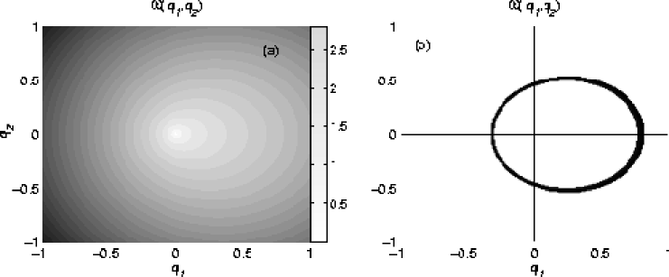
Figure 2: (a). Contour plot of $\omega({\bf q})$. Each grayscale corresponds to a different constant value of $\omega({\bf q})=\omega({\bf k})\equiv\omega_{0}$. (b). The band of ${\bf q}$ that satisfies $0.625<\omega_{0}<0.6625$. Wavevectors ${\bf q}$ and ${\bf k}$ that lie in this band can couple $a({\bf x},{\bf k},t)$ to $a({\bf x},{\bf q},t)$ via wave scattering.

Each grayscale corresponds to a curve defined by fixed $\omega({\bf k})=\omega_{0}$. All wavevectors ${\bf q}$ in each contour contribute to the integration in the expressions for $\Sigma({\bf k})$ and $\omega({\bf q},{\bf k})$. Thus, slowly varying drift can induce an indirect doppler coupling between waves with different wavenumbers, with the most drastic coupling occurring at the two far ends of a particular oval curve. For example, in Figure 2(b), the dark band denotes ${\bf q}$ such that $\omega({\bf q})=\omega_{0}$ when $0.625<\omega_{0}<0.6625$. The wavevectors ${\bf q}\approx(-0.3,0)$ and ${\bf q}\approx(0.8,0)$ are two of many that contribute to the scattering terms. Therefore, the evolution of $a({\bf x},{\bf k}\approx(-0.3,0),t)$ also depends on $a({\bf x},{\bf q}\approx(0.8,0),t)$ via the second term on the right side of (35).

Provided ${\bf U}({\bf x})$ is sufficiently large, the $\tau=-1$ terms can also contribute to scattering. The dissipative scattering rate $\Sigma({\bf k})a({\bf x},{\bf k},t)$ will change quantitatively since additional ${\bf q}$’s will contribute to $\Sigma({\bf k})$. However, this decay process depends only on ${\bf k}$ and is not coupled to $a({\bf x},|{\bf q}|\neq|{\bf k}|,t)$. Wavevectors ${\bf q}$ that satisfy the $\delta-$function in the $\sigma({\bf q},{\bf k})a({\bf x},{\bf q},t)$ term will, as when $\tau=+1$, lead to indirect doppler coupling. This occurs when $\omega({\bf q})=-\omega_{0}$ and, as we shall see, allows doppler coupling of waves with more widely varying wavelengths than compared to the $\tau=+1$ case. Observe that if $\tau=-1$ terms arise, the drift frame energy $a({\bf x},{\bf k},t)\omega({\bf x},{\bf k})$ is no longer conserved. Figure 3(a) plots $\omega(q_{1},q_{2}=0)$ for $U({\bf x})=1<\sqrt{2},U({\bf x})=\sqrt{2}$, and $U({\bf x})=1.6>\sqrt{2}$. Since $\omega_{0}$ and $\omega({\bf q})$ are identical functions, $-\omega_{0}$ can take on values below the upper dotted line ($\omega_{0}\lesssim 0.22$ for $U=1.6$). Therefore, coupling for $\tau=-1$ and $q_{2}=0$ occurs for values of $-\omega_{0}$ between the dotted lines. Note that depending upon the value of $\omega_{0}$, coupling can occur at two or four different points ${\bf q}=(q_{1},0)$. Figure 3(b) shows a contour plot of $|\omega({\bf q})|$ as a function of $(q_{1},q_{2})$. A level set lying between the dotted lines in $(a)$ will slice out two bands; one band corresponds to all values of ${\bf k}$ that couple to ${\bf q}$ lying in the associated second band. The two bands determined by the interval $0.414<-\omega_{0}<0.468$ are shown in Fig. 3(c). For any ${\bf k}$ lying in the inner band of Fig. 3(c), all ${\bf q}$ lying in the outer band will contribute to doppler coupling for $\tau=-1$, and vice versa. As $-\omega_{0}$ is increased, the inner(outer) band decreases(increases) in size, with the central band vanishing when $-\omega_{0}$ approaches the upper dotted line in $(a)$ where the $\tau=-1$ coupling evaporates. If $-\omega_{0}$ is decreased, the two bands merge, then disappear as $-\omega_{0}$ reaches the lower limit. Fig. 3(d) is an expanded view of the two bands for small $0.0756<-\omega_{0}<0.1368$. Note that a small island of ${\bf q}$ or ${\bf k}$ appears for very small wavevectors. The water wave scattering represented by $\sigma({\bf q},{\bf k})$ can therefore couple very long wavelength modes with very short wavelength modes (the two larger bands to the right in Fig. 3(d)). However, the strength of this coupling is still determined by the magnitude of $q_{i}R_{ij}(|{\bf q}-{\bf k}|)k_{j}$, which may be small for $|{\bf q}-{\bf k}|$ large.

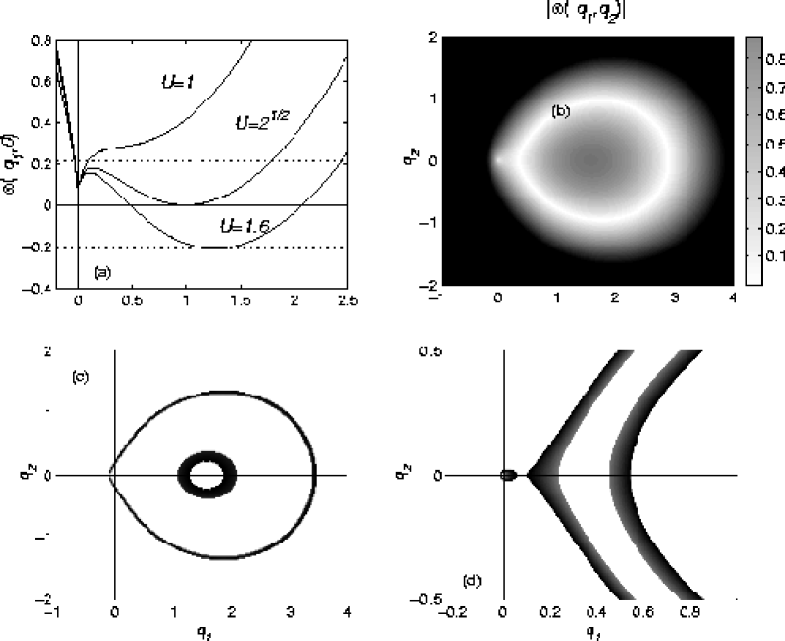
Figure 3: Conditions for doppler coupling when $\tau=-1$. (a). Plot of $\omega(q_{1},q_{2}=0;h=\infty)$ for $U=1$, $U=\sqrt{2}$, and $U=1.6$. Only for $U>\sqrt{2}$ does $\omega(q_{1},q_{2}=0;h=\infty)<0$. (b). Contour plot of $|\omega({\bf q})|$. Each grayscale corresponds to a different constant value of $\omega({\bf q})=\omega({\bf k})\equiv-\omega_{0}$. (c). The bands of ${\bf q}$ satisfying $0.414<-\omega_{0}<0.468$. (d). An expanded view of the coupling bands for $0.0756<-\omega_{0}<0.1368$. Note that wavenumbers of very small modulus can couple with wavenumbers of significantly larger modulus.

The depth dependence of doppler coupling will be relevant when $hq,hk\lesssim 1$ where $q$ and $k$ are the magnitudes of the wavevectors of two doppler-coupled waves. For $\tau=+1$, finite depth reduces the ellipticity of the coupling bands, resulting in weaker doppler effects. Since the water wave phase velocity decreases with $h$, a finite depth will also reduce the critical $U({\bf x})$ required for $\tau=-1$ doppler coupling. For small $U({\bf x})$, it is clear that the $\delta-$functions associated with the $\tau=-1$ terms in $\sigma({\bf q},{\bf k})$ are first triggered when the ${\bf q}$ and ${\bf k}$ are antiparallel, ${\bf U}\cdot{\bf k}=-k|{\bf U}|,{\bf U}\cdot{\bf q}=+q|{\bf U}|$.

Figure 4(a) shows the phase velocity for various depths $h$. In order for $\tau=-1$ to contribute to scattering, $U\geq c_{\phi}(k;h)$. For $U\approx 1.6$, this condition holds in the $h=\infty$ case for $0.5\lesssim k\lesssim 2$ (the dashed region of $c_{\phi}(k,\infty)$). Recall that our starting equations (4) are valid only in the small Froude number limit. However, for water waves propagating over infinite depth, $\tau=-1$ coupling requires $U>U_{min}=\mbox{min}_{k}\{c_{\phi}(k)\}$, with $c_{\phi}(k_{min})\simeq 22$cm/s. Therefore, in such “supersonic” cases, where $\tau=-1$ is relevant, our treatment is accurate only at wavevectors $k^{*}$ such that $U\ll c_{\phi}(k^{*};h)$, e.g., the thick solid portion of $c_{\phi}(k;\infty)$. For $U\gtrsim U_{min}$, the $\tau=-1$ term can couple wavevectors $q\approx 0\ll k_{min}$ with $k\approx 2-3\gg k_{min}$. The rich $\tau=-1$ doppler coupling displayed in Figures 3 is particular to water waves with a dispersion relation $\omega({\bf q})$ that behaves as $q^{3/2},{\bf U}\cdot{\bf q}$, or $q^{1/2}$ depending on the wavelength. Doppler coupling in water wave propagation is very different from that arising in acoustic wave propagation in an incompressible, randomly flowing fluid ([Howe (1973), Fannjiang & Ryzhik (1999), Vedantham & Hunter (1997)]) where $\omega({\bf q})=c_{s}|{\bf q}|$. An additional doppler coupling analogous to the $\tau=-1$ coupling for water waves arises only for supersonic random flows when $U({\bf x})\geq c_{s}$, independent of $q$. In such instances, compressibility effects must also be considered.

Figure 4(b) plots the minimum drift velocity $U_{min}(h)$ where $\tau=-1$ doppler coupling first occurs at any wavevector. The wavevector at which coupling first occurs is also shown by the dashed curve. For shallow water, $h\ll\sqrt{3}$, $U_{min}(h)\propto\sqrt{h}$ and very long wavelengths couple first (small $k(U_{min})$). For depths $h>\sqrt{3}$ ($\sim 3$cm for water), the minimum drift required quickly increases to $U^{*}(\infty)=\sqrt{2}$, while the initial coupling occurs at increasing wavevectors until at infinite depth, where the first wavevector to doppler couple approaches $k\rightarrow 1$ (in water, this corresponds to wavelengths of $\sim 6.3$cm). The conditions for $\tau=-1$ doppler coupling outlined in Figures 2 and 3 apply to both $\Sigma({\bf k})$ and $\sigma({\bf q},{\bf k})$, with the proviso that ${\bf q}$ and ${\bf k}$ are parallel for $\Sigma({\bf k})$ and antiparallel for $\sigma({\bf q},{\bf k})$. However, even when $U<U_{min}$ such that only $\tau=+1$ applies, the set of ${\bf q}$ corresponding to a constant value of $\omega({\bf k})=\omega_{0}$, traces out a noncircular curve. There is doppler coupling between wavenumbers $q\neq k$ as long as $U\neq 0$.

Figure 4: $U>c_{\phi}(k)$ is required for $\tau=-1$ coupling. (a). The phase velocity $c_{\phi}(k)$ for various depths $h$. The velocity shown by the solid horizontal line $U\approx 1.6>c_{\phi}(k;h=\infty)$ for $0.5\lesssim k\lesssim 2$. (b). The minimum $U_{min}(h)$ required for existence of $\tau=-1$ coupling at any wavevector $k$, and the wavevector $k(U_{min})$ at which this first happens.

5.4 Surface wave diffusion

We now consider the radiative transfer equation (35) over propagation distances long compared to the mean free path $\ell_{\mbox{{\it mfp}}}$. Imposing an additional rescaling and measuring all distances in terms of the mean free path, we introduce another scaling $\epsilon^{-1}$, proportional to the number of mean free paths travelled. Since $\beta=1/2$, transport of wave action prevails when $O(\varepsilon)<|{\bf x}|\sim O(1)$, while diffusion holds when $O(\epsilon^{-1})\sim|{\bf x}|<\ell_{\mbox{\it loc}}$.

Since waves of each frequency satisfy (35) independently, we consider the diffusion of waves of constant frequency $\omega_{0}$. To derive the diffusion equation, we assume for simplicity that ${\bf U}$ is constant and small such that $\omega_{0}+\omega({\bf x},{\bf q})\neq 0$ (the $\tau=-1$ terms are never triggered by the $\delta-$functions). Expanding all quantities in the transport equation (35) in powers of $\epsilon$, we find

$$\dot{a}_{0}+\bar{\bf U}\cdot\nabla_{\bf x}a_{0}-\nabla_{\bf x}\cdot{\bf D}\cdot\nabla_{\bf x}a_{0}=0.$$ (55)

The derivation of this equation is given in Appendix B. The diffusion tensor ${\bf D}$ is given in (77) and is a function of the power spectrum $R_{ij}$. The effective drift $\bar{\bf U}$ is given by (72):

$$\bar{\bf U}=\frac{\int_{\bf k}\nabla_{\bf k}\omega({\bf k})\delta({\bf k}\cdot{\bf U}+\Omega({\bf k})-\omega_{0})}{\int_{\bf k}\delta({\bf k}\cdot{\bf U}+\Omega({\bf k})-\omega_{0})}.$$ (56)

Up to a change of basis, we can assume that ${\bf U}=U{\bf e}_{1}$, where $U>0$. Then the set of points ${\bf k}\cdot{\bf U}+\Omega({\bf k})-\omega_{0}=0$ is symmetric with respect to the $x_{1}-$axis and $\bar{\bf U}$ is parallel to ${\bf U}$. Also notice that the total energy given in (27) is asymptotically conserved in the diffusive regime. Indeed, the total energy variations are given by (53). Assuming that all water waves have frequency $\omega_{0}$, we have in the diffusive regime

$$\begin{array}[]{rcl}\displaystyle\frac{d}{dt}{\cal E}&=&-\displaystyle\frac{d}{dt}\displaystyle\int_{\bf x}\displaystyle\int_{\bf k}{\bf k}\cdot{\bf U}({\bf x})\,a({\bf x},{\bf k},t)\\ &\approx&-\Big{(}\displaystyle\int_{\bf x}\dot{a}_{0}({\bf x},t)\Big{)}\displaystyle\int_{\bf k}{\bf k}\cdot{\bf U}\delta(\omega_{0}-\omega({\bf k})),\\ \end{array}$$

since ${\bf U}$ is constant. Recasting the diffusion equation as $\dot{a}_{0}=-\nabla_{\bf x}\cdot(\bar{\bf U}a_{0}+{\bf D}\cdot\nabla_{\bf x}a_{0})$, we deduce that

$$\int_{\bf x}\dot{a}_{0}({\bf x},t)=0,$$

which conserves the total energy ${\cal E}$.

Now consider the simplified case ${\bf U}\equiv 0$, $h=\infty$ and $\Omega_{\infty}({\bf k})=\sqrt{k^{3}+k}$. Since ${\bf U}=\bar{{\bf U}}=0$, (54) holds and we have for all ${\bf k}$,

$$\int_{\bf q}q_{i}R_{ij}(|{\bf q}-{\bf k}|)q_{j}{\bf q}=\bf{0}.$$ (57)

We deduce that the corrector $\boldsymbol{\chi}$ in (73) is given by

$$\boldsymbol{\chi}({\bf k})=-\frac{\nabla_{\bf k}\Omega_{\infty}({\bf k})}{\Sigma(k)}=-\frac{|\nabla_{\bf k}\Omega_{\infty}({\bf k})|}{\Sigma(k)}\hat{\bf k}=-\frac{c_{g}}{\Sigma(k)}\hat{\bf k},$$

where ${\bf k}=k\hat{{\bf k}}$. The isotropic diffusion tensor ${\bf D}$ is thus given by

$${\bf D}=\frac{1}{\Sigma(k)V_{\omega_{0}}}\int_{\bf q}|\nabla_{\bf q}\Omega_{\infty}({\bf q})|^{2}\hat{\bf q}\hat{\bf q}^{T}\delta(\Omega_{\infty}({\bf q})-\omega_{0})=\frac{c_{g}^{2}(k)}{2\Sigma(k)}\,\,{\bf I},$$ (58)

where ${\bf I}$ is the $2\times 2$ identity matrix. Thus, the diffusion equation for $a_{0}({\bf x},t)$ assumes the standard form ([Sheng (1995)])

$$\dot{a}_{0}-\frac{c_{g}^{2}(k)}{2\Sigma(k)}\Delta a_{0}=0.$$ (59)

6 Summary and Conclusions

In this paper, we have used the Wigner distribution to derive the transport equations for water wave propagation over a spatially random drift composed of a slowly varying part ${\bf U}({\bf x})$, and a rapidly varying part $\sqrt{\varepsilon}\delta{\bf U}({\bf x}/\varepsilon)$. The slowly varying part determines the characteristics on which the waves propagate. We recover the standard result obtained from WKB theory: conservation of wave action. Provided $R_{ij}({\bf q})q_{j}=0$, we extend CWA to include wave scattering from correlations $R_{ij}$ of the rapidly varying random flow. Evolution equations for the nonconserved wave intensity and energy density can be readily obtained from (35). Moreover, conservation of drift frame energy $a({\bf x},{\bf k},t)\omega({\bf x},{\bf k})$ requires small $U<U_{min}$ and absence of $\tau=-1$ contributions to scattering.

Explicit expressions for the scattering rates $\Sigma({\bf k})$ and $\sigma({\bf q},{\bf k})$ are given in Eqs. (37). For fixed $\omega({\bf k})$, we find the set of ${\bf q}$ such that the $\delta-$functions in (37) are supported. This set of ${\bf q}$ indicates the wavevectors of the background surface flow that can mediate doppler coupling of the water waves. Although widely varying wavenumbers can doppler couple, supported by the $\delta-$function constraints, particularly for $\tau=-1$, the correlation $R_{ij}(|{\bf q}-{\bf k}|)$ also decreases for large $|{\bf q}-{\bf k}|$. For long times, multiple weak scattering nonetheless exchanges action among disparate wavenumbers within the transport regime. Our collective results, including water wave action diffusion, provide a model for describing linear ocean wave propagation over random flows of different length scales. The scattering terms in (35) also provide a means to correlate sea surface wave spectra to statistics $R_{ij}$ of finer scale random flows.

Although many situations arise where the underlying flow is rotational ([White (1999)]), the irrotational approximation used simplifies the treatment and allows a relatively simple derivation of the transport and diffusive regimes of water wave propagation. The recent extension by [White (1999)] of CWA to include rotational flows also suggests that an explicit consideration of velocity and pressure can be used to generalise the present study to include rotational random flows. Other feasible extensions include the analysis of a time varying random flow, as well as separating the underlying flows into static and wave dynamic components.

Appendix A Derivation of the transport equation

Some of the steps in the derivation of (35) are outlined here. By taking the time derivative of $W_{ij}$ in (14) and using the definition (17) for $\dot{\psi}$, we obtain

$$\begin{array}[]{rl}\displaystyle(2\pi\varepsilon)^{2}\dot{W}_{ij}({\bf p},{\bf k},t)&\displaystyle=(2\pi\varepsilon)^{2}iW_{i\ell}({\bf p},{\bf k})L_{\ell j}^{*}\left({{\bf k}\over\varepsilon}-{{\bf p}\over 2}\right)-(2\pi\varepsilon)^{2}iL_{i\ell}\left({{\bf k}\over\varepsilon}+{{\bf p}\over 2}\right)W_{\ell j}({\bf p},{\bf k})\\[13.0pt] &\displaystyle+i\int_{{\bf q}}{\bf U}({\bf q})\cdot\left(-{{\bf k}\over\varepsilon}+{{\bf p}\over 2}-{\bf q}\delta_{i2}\right)\psi_{i}\left(-{{\bf k}\over\varepsilon}+{{\bf p}\over 2}-{\bf q}\right)\psi_{j}^{*}\left(-{{\bf k}\over\varepsilon}-{{\bf p}\over 2}\right)\\[13.0pt] &\displaystyle-i\int_{{\bf q}}{\bf U}^{*}({\bf q})\cdot\left(-{{\bf k}\over\varepsilon}-{{\bf p}\over 2}-{\bf q}\delta_{j2}\right)\psi_{i}\left(-{{\bf k}\over\varepsilon}+{{\bf p}\over 2}\right)\psi_{j}^{*}\left(-{{\bf k}\over\varepsilon}-{{\bf p}\over 2}-{\bf q}\right)\\[13.0pt] &\displaystyle+i\sqrt{\varepsilon}\int_{{\bf q}}\delta{\bf U}({\bf q})\cdot\left(-{{\bf k}\over\varepsilon}+{{\bf p}\over 2}-{{\bf q}\over\varepsilon}\delta_{i2}\right)\psi_{i}\left(-{{\bf k}\over\varepsilon}+{{\bf p}\over 2}-{{\bf q}\over\varepsilon}\right)\psi_{j}^{*}\left(-{{\bf k}\over\varepsilon}-{{\bf p}\over 2}\right)\\[13.0pt] &\displaystyle-i\sqrt{\varepsilon}\int_{{\bf q}}\delta{\bf U}^{*}({\bf q})\cdot\left(-{{\bf k}\over\varepsilon}-{{\bf p}\over 2}-{{\bf q}\over\varepsilon}\delta_{j2}\right)\psi_{i}\left(-{{\bf k}\over\varepsilon}+{{\bf p}\over 2}\right)\psi_{j}^{*}\left(-{{\bf k}\over\varepsilon}-{{\bf p}\over 2}-{{\bf q}\over\varepsilon}\right)\end{array}$$ (60)

To rewrite the above expression as a function of $W_{ij}$ only, we relabel appropriately, e.g.,

$$\begin{array}[]{rl}\displaystyle-{{\bf k}\over\varepsilon}-{{\bf p}\over 2}&\displaystyle=-{{\bf k}^{\prime}\over\varepsilon}-{{\bf p}^{\prime}\over 2}\\[13.0pt] \displaystyle-{{\bf k}\over\varepsilon}+{{\bf p}\over 2}-{\bf q}&\displaystyle=-{{\bf k}^{\prime}\over\varepsilon}+{{\bf p}^{\prime}\over 2}\end{array}$$ (61)

for the third term on the right hand side of (60). Similarly relabelling for all relevant terms yields the integral equation (19).

The $O(\varepsilon^{-1/2})$ terms of (19) determine ${\bf W}_{1/2}$. Decomposing

$${\bf W}_{1/2}({\bf p},\boldsymbol{\xi},{\bf k})\equiv\sum_{\tau,\tau^{\prime}=\pm}a^{(1/2)}_{\tau,\tau^{\prime}}({\bf p},\boldsymbol{\xi},{\bf k}){\bf b}_{\tau}({\bf k}_{-}){\bf b}_{\tau^{\prime}}^{\dagger}({\bf k}_{+})$$ (62)

and substituting into (31) we find the coefficients $a_{\tau,\tau^{\prime}}^{(1/2)}$, where in this case $a_{+-}^{(1/2)},a_{-+}^{(1/2)}\neq 0$. Due to the nonlocal nature of the third term on the right of (31), we must first inverse Fourier transform the slow wavevector variable back to ${\bf x}$.

To extract the $O(\varepsilon^{0})$ terms from (19) we need to expand ${\bf L}$ to order $\varepsilon^{0}$, the ${\bf L}_{1}$ term. Similarly, the terms ${\bf W}({\bf p}-{\bf q},\boldsymbol{\xi},{\bf k}\pm\varepsilon{\bf q}/2)$ must be expanded:

$${\bf W}({\bf p}-{\bf q},\boldsymbol{\xi},{\bf k}\pm\varepsilon{\bf q}/2)={\bf W}({\bf p}-{\bf q},\boldsymbol{\xi},{\bf k})\pm{\varepsilon\over 2}{\bf q}\cdot\nabla_{{\bf k}}{\bf W}({\bf p}-{\bf q},\boldsymbol{\xi},{\bf k})+O(\varepsilon^{2}).$$ (63)

The $\varepsilon{\bf q}\cdot\nabla_{{\bf k}}{\bf W}({\bf p}-{\bf q},\boldsymbol{\xi},{\bf k})$ terms combine with the $-\varepsilon^{-1}{\bf U}({\bf q})\cdot{\bf k}_{-}+\varepsilon^{-1}{\bf U}({\bf q})\cdot{\bf k}_{+}$ terms from the third and fourth terms in (19) to give the third term on the right of Eq. (34). The $\delta{\bf U}$-dependent, order $\varepsilon^{0}$ terms (the sixth, seventh, and eighth terms on the right side of (34)) come from collecting

$$\pm\sqrt{\varepsilon}\delta{\bf U}({\bf q})\cdot\left(-{{\bf k}\over\varepsilon}\pm{\boldsymbol{\xi}\over 2\varepsilon}\right)\sqrt{\varepsilon}{\bf W}_{1/2}({\bf p},\boldsymbol{\xi}-{\bf q},{\bf k}\pm{\bf q}/2)$$ (64)

from the last two terms in (19). The ensemble averaged time evolution of the Wigner amplitude $a_{\sigma}({\bf x},{\bf k})$ can be succinctly written in the form:

$$\begin{array}[]{l}\dot{a}_{+}({\bf x},{\bf k},t)-\nabla_{{\bf x}}\omega({\bf x},{\bf k})\cdot\nabla_{{\bf k}}a_{+}({\bf x},{\bf k},t)+\nabla_{{\bf k}}\omega({\bf x},{\bf k})\cdot\nabla_{{\bf x}}a_{+}({\bf x},{\bf k},t)\\[13.0pt] \>\hskip 144.54pt=\displaystyle\Sigma_{+,\mu}({\bf k})a_{\mu}({\bf x},{\bf k},t)+\int_{{\bf q}}\sigma_{+,\mu}({\bf q},{\bf k})a_{\mu}({\bf x},{\bf k},t).\end{array}$$ (65)

Using the form for ${\bf W}_{0}$ found from (23) in (31) to find ${\bf W}_{1/2}$, we substitute into (34) to find (35), the transport equation for one of the diagonal intensities of the Wigner distribution. We have explicitly used eigenbasis orthonormality ${\bf b}_{\tau}^{\dagger}({\bf k})\cdot{\bf c}_{\tau^{\prime}}({\bf k})=\delta_{\tau,\tau^{\prime}}$ and the fact that $a_{-}({\bf x},{\bf k},t)=a_{+}({\bf x},-{\bf k},t)$.

Appendix B Derivation of the diffusion equation

The derivation of diffusion of water wave action is outlined below and follows the established mathematical treatment of [Larsen & Keller (1974)] and [Dautray & Lions (1993)]. For simplicity we assume that the flow ${\bf U}$ is constant and small enough so that for a considered range of frequencies, the relation $\omega({\bf q})+\omega({\bf k})=0$ is never satisfied for any ${\bf k}$ and ${\bf q}\neq{\bf 0}$. The diffusion approximation is valid after long times and large distances of propagation ${\bf X}$(see Fig. 1) such that the wave has multiply scattered and its dynamics are determined by a random walk. We therefore rescale time and space as

$$\tilde{t}=\frac{t}{\epsilon^{2}},\qquad\tilde{\bf x}=\frac{{\bf x}}{\epsilon}.$$ (66)

The small parameter $\epsilon$ in this further rescaling represents the transport mean free path $\ell_{\mbox{{\it mfp}}}$ and not the wavelength as in the initial rescaling used to derive the transport equation. We drop the tilde symbol for convenience and rewrite the transport equation in the new variables:

$$\dot{a}_{\epsilon}({\bf x},{\bf k},t)+\frac{1}{\epsilon}\nabla_{\bf k}\omega({\bf k})\cdot\nabla_{\bf x}a_{\epsilon}({\bf x}.{\bf k},t)=\frac{1}{\epsilon^{2}}\int_{{\bf q}}{\cal Q}({\bf q},{\bf k})(a_{\epsilon}({\bf x},{\bf q},t)-a_{\epsilon}({\bf x},{\bf k},t))\delta(\omega({\bf q})-\omega({\bf k})),$$ (67)

with obvious notation for ${\cal Q}({\bf q},{\bf k})$. Since the frequency is fixed, the equation is posed for ${\bf k}$ satisfying $\omega({\bf k})=\omega_{0}$. The transport equation assumes the form (67) because the scattering operator is conservative. Since ${\bf U}\neq 0$, wave action is transported by the flow, and diffusion takes place on top of advection. Therefore, we introduce the main drift $\bar{\bf U}$, which will be computed explicitly later, and define the drift-free unknown $\tilde{a}_{\epsilon}({\bf x},{\bf k},t)$ as

$$\tilde{a}_{\epsilon}({\bf x},{\bf k},t)=a_{\epsilon}({\bf x}+\frac{\bar{\bf U}}{\epsilon}t,{\bf k},t).$$ (68)

It is easy to check that $\tilde{a}_{\epsilon}$ satisfies the same transport equation as $a_{\epsilon}$ where the drift term $\nabla_{\bf k}\omega$ has been replaced by $\nabla_{\bf k}\omega-\bar{\bf U}$.

We now derive the limit of $\tilde{a}_{\epsilon}$ as $\epsilon\to 0$. Consider the classical asymptotic expansion

$$\tilde{a}_{\epsilon}=\tilde{a}_{0}+\epsilon\tilde{a}_{1}+\epsilon^{2}\tilde{a}_{2}+\ldots.$$ (69)

Upon substitution into (67) and equating like powers of $\epsilon$, we obtain at order $\epsilon^{-2}$, for fixed frequency $\omega_{0}$,

$$\int_{{\bf q}}{\cal Q}({\bf q},{\bf k})(\tilde{a}_{0}({\bf x},{\bf q},t)-\tilde{a}_{0}({\bf x},{\bf k},t))\delta(\omega({\bf q})-\omega_{0})=0.$$ (70)

It follows from the Krein-Rutman theory ([Dautray & Lions (1993)]) that $\tilde{a}_{0}$ is independent of ${\bf q}$. At order $\epsilon^{-1}$, we obtain

$$(\nabla_{\bf k}\omega({\bf k})-\bar{\bf U})\cdot\nabla_{\bf x}\tilde{a}_{0}=\int_{{\bf q}}{\cal Q}({\bf q},{\bf k})(\tilde{a}_{1}({\bf x},{\bf q},t)-\tilde{a}_{1}({\bf x},{\bf k},t))\delta(\omega({\bf q})-\omega_{0}).$$ (71)

The compatibility condition for this equation to admit a solution requires both sides to vanish upon integration over $\delta(\omega({\bf k})-\omega_{0})d{\bf k}$. Therefore, $\bar{\bf U}$ satisfies

$$\bar{\bf U}=\frac{1}{V_{\omega_{0}}}\int_{\bf k}\nabla_{\bf k}\omega({\bf k})\delta(\omega({\bf k})-\omega_{0}),\qquad\mbox{ where }\qquad V_{\omega_{0}}=\int_{\bf k}\delta(\omega({\bf k})-\omega_{0}).$$ (72)

Once the constraint is satisfied, we deduce from Krein-Rutman theory the existence of a vector-valued mean zero corrector $\boldsymbol{\chi}$ solving

$$(\nabla_{\bf k}\omega({\bf k})-\bar{\bf U})=\int_{{\bf q}}{\cal Q}({\bf q},{\bf k})(\boldsymbol{\chi}({\bf q})-\boldsymbol{\chi}({\bf k}))\delta(\omega({\bf q})-\omega_{0})\equiv{\cal L}\boldsymbol{\chi}.$$ (73)

There is no general analytic expression for $\boldsymbol{\chi}$, which must in practice be solved numerically. This is typical of problems where the domain of integration in ${\bf q}$ does not have enough symmetries (cf. [Allaire & Bal (1999), Bal (1999)]). We now have

$$\tilde{a}_{1}({\bf x},{\bf k},t)=\boldsymbol{\chi}({\bf k})\cdot\nabla_{\bf x}\tilde{a}_{0}({\bf x},t).$$ (74)

It remains to consider $O(\epsilon^{0})$ in the asymptotic expansion. This yields

$$\dot{\tilde{a}}_{0}+(\nabla_{\bf k}\omega({\bf k})-\bar{\bf U})\cdot\nabla_{\bf x}\tilde{a}_{1}={\cal L}(\tilde{a}_{2}).$$ (75)

The compatibility condition, obtained by integrating both sides over ${\bf k}$, yields the wave action diffusion equation

$$\dot{\tilde{a}}_{0}-\nabla_{\bf x}\cdot{\bf D}\cdot\nabla_{\bf x}\tilde{a}_{0}=0,$$ (76)

where the diffusion tensor is given by

$${\bf D}=-\frac{1}{V_{\omega_{0}}}\int_{\bf k}(\nabla_{\bf k}\omega({\bf k})-\bar{\bf U})\boldsymbol{\chi}^{T}({\bf k})=-\frac{1}{V_{\omega_{0}}}\int_{\bf k}{\cal L}(\boldsymbol{\chi})\boldsymbol{\chi}^{T}({\bf k}).$$ (77)

The second form shows that ${\bf D}$ is positive definite since ${\cal L}$ is a nonpositive operator. The formal asymptotic expansion can be justified rigorously using the techniques in [Dautray & Lions (1993)]. As $\epsilon\to 0$, we obtain that the error between $\tilde{a}_{\epsilon}$ and $\tilde{a}_{0}$ is at most of order $\epsilon$. Therefore, we have that $a_{\epsilon}$ converges to $a_{0}$ satisfying the following drift-diffusion equation

$$\dot{a}_{0}+\frac{\bar{\bf U}}{\epsilon}\cdot\nabla_{\bf x}a_{0}-\nabla_{\bf x}\cdot{\bf D}\cdot\nabla_{\bf x}a_{0}=0,$$ (78)

with suitable initial conditions. Equation (78) is the coordinate-scaled version of (55).

References

• [Allaire & Bal (1999)] Allaire G. & Bal, G. 1999 Homogenization of the criticality spectral equation in neutron transport M2AN Math. Model. Numer. Anal. 33 721-746.
• [Bal (1999)] Bal, G. 1999 First-order Corrector for the Homogenization of the Criticality Eigenvalue Problem in the Even Parity Formulation of the Neutron Transport SIAM J. Math. Anal. 30 1208-1240.
• [Bal et al. (1999)] Bal, G., Fannjiang, A., Papanicolaou, G. & Ryzhik, L. 1999 Radiative Transport in a Periodic Structure J. Stat. Phys. 95 479-494.
• [Bender & Orszag (1978)] Bender, C. M., & Orszag, S. A. 1978 Advanced Mathematical Methods for Scientists and Engineers. (McGraw-Hill, New York).
• [Cerda & Lund (1993)] Cerda, E. & Lund, F. 1993 Interaction of surface waves with vorticity in shallow water Phys. Rev. Lett. 70 3896-3899.
• [Chou (1998)] Chou, T. 1998 Band structure of surface flexural-gravity waves along periodic interfaces J. Fluid Mech. 369 333-350.
• [Chou, Lucas & Stone (1995)] Chou, T., Lucas, S. K., & Stone, H. A. 1995 Capillary Wave Scattering from a Surfactant Domain Phys. Fluids 7 1872-1885.
• [Chou & Nelson (1994)] Chou, T., & Nelson, D. R. 1994 Surface Wave Scattering from Nonuniform Interfaces J. Chem. Phys. 101 9022-9031.
• [Courant & Hilbert (1962)] Courant, R. & Hilbert, D., Methods of Mathematical Physics, Vol. II. Wiley Interscience.
• [Dautray & Lions (1993)] Dautray, R. & Lions, J.-L., Mathematical Analysis and Numerical Methods for Science and Technology. Vol.6, Springer Verlag, Berlin.
• [Elter & Molyneux (1972)] Elter, J. F. & Molyneux, J. E. 1972 The long-distance propagation of shallow water waves over an ocean of random depth J. Fluid Mech. 53 1-15.
• [Erdös & Yau (1998)] Erdös, L. & Yau, H.T. 1998 Linear Boltzmann equation as scaling limit of quantum Lorentz gas Advances in Differential Equations and Mathematical Physics. Contemporary Mathematics 217 136-155.
• [Fabrikant & Raevsky (1994)] Fabrikant, A. L. & Raevsky, M. A. 1994 Influence of drift flow turbulence on surface gravity-wave propagation J. Fluid Mech. 262, 141-156.
• [Fannjiang & Ryzhik (1999)] Fannjiang, A. & Ryzhik, L. 1999 Phase space transport for sound waves in random flows Submitted to SIAM.
• [Gerber (1993)] Gerber, M. 1993 The interaction of deep-gravity waves and an annular current: linear theory. J. Fluid Mech. 248, 153-172.
• [Gou, Messiter & Schultz (1993)] Gou, S., Messiter, A. F. & Schultz, W. W. 1993 Capillary-gravity waves in a surface tension gradient. I: Discontinuous change. Phys. Fluids A 5, 966-972.
• [Gérard et al. (1997)] Gérard, P., Markowich, P. A., Mauser, N.J., & Poupaud, F. 1997 Homogenization limits and Wigner transforms Comm. Pure Appl. Math. 50, 323-380.
• [Henyey et al. (1988)] Henyey, F. S., Creamer, D. B., Dysthe, K. B., Schult, R. L., & Wright, J. A. 1988 The energy and action of small waves riding on large waves J. Fluid Mech. 189, 443-462.
• [Howe (1973)] Howe, M. 1973 Multiple scattering of sound by turbulence and other inhomogeneities J. Sound and Vibration 27, 455-476.
• [Jonsson (1990)] Jonsson, I.G. 1990 Wave-current interactions Ocean Engineering Science: The Sea (ed. B. Le Mehaute & D. Hanes), 65-120, Wiley.
• [Keller (1958)] Keller, J. B. 1958 Surface Waves on water of non-uniform depth J. Fluid Mech. 4, 607-614.
• [Kleinert (1990)] Kleinert, P. 1990 A field-theoretical treatment of Third-Sound localization Phys. Stat. Sol. B 158, 539-550.
• [Lee et al. (1993)] Lee, K. Y., Chou, T., Chung, D. S. & Mazur, E. 1993 Direct Measurement of the Spatial Damping of Capillary Waves at Liquid-Vapor Interfaces J. Phys. Chem. 97, 12876-12878.
• [Landau (1985)] Landau 1985 Fluid Mechanics. Pergamon.
• [Larsen & Keller (1974)] Larsen, E. W. & Keller, J. B. 1974 Asymptotic solution of neutron transport problems for small mean free paths J. Math. Phys. 15, 75-81.
• [Longuet-Higgins & Stewart (1961)] Longuet-Higgins, M. S. & Stewart, R. W. 1961 The changes in amplitude of short gravity waves on steady non-uniform currents J. Fluid Mech. 10, 529-549.
• [Mei (1979)] Mei, C. C. 1979 The Applied Dynamics of Ocean Surface Waves. Wiley Interscience.
• [Naciri & Mei (1988)] Naciri, M, & Mei, C. C. 1988 Bragg scattering of water waves by a doubly periodic seabed. J. Fluid Mech. 192, 51-74.
• [Naciri & Mei (1992)] Naciri, M, & Mei, C. C. 1992 Evolution of a short surface wave on a very long surface wave of finite amplitude. J. Fluid Mech. 235, 415-452.
• [Peregrine (1976)] Peregrine, D.H. 1976 Interaction of water waves and currents. Adv. Appl. Mech. 16, 9-117.
• [Rayevskiy (1983)] Rayevskiy, M. A. 1983 On the propagation of gravity waves in randomly inhomogeneous nonsteady-state currents. Izvestiya, Atmos. & Oceanic Phys. 19, 475-479.
• [Ryzhik, Papanicolaou, & Keller (1996)] Ryzhik, L. V., Papanicolaou, G. C., & Keller, J. B. 1996 Transport equations for elastic and other waves in random media Wave Motion 24, 327-370.
• [Sheng (1995)] Sheng, P. 1995 Introduction to Wave Scattering, Localization, and Mesoscopic Phenomena. Academic Press.
• [Spohn (1977)] Spohn, H. 1977 Derivation of the Transport Equation for Electrons Moving Through Random Impurities. J. Stat. Phys. 17, 385-412.
• [Trulson & Mei (1993)] Trulsen, K. and Mei, C. C. 1993 Double reflection of capillary/gravity waves by a non-uniform current: a boundary layer theory. J. Fluid Mech. 251, 239-271.
• [Vedantham & Hunter (1997)] Vedantham, R. & Hunter, J. 1997 Sound wave propagation through incompressible flows Wave Motion 26, 319-328.
• [White (1999)] White, B. S. 1999 Wave action on currents with vorticity. J. Fluid Mech. 386, 329-344.
• [Whitham (1974)] Whitham, G. B. 1974 Linear & Nonlinear waves. Wiley Interscience.
• [Wigner (1932)] Wigner, E. 1932 On the quantum correction for thermodynamic equilibrium. Phys. Rev. 40, 742-749.
• [Zakharov, L’vov & Falkovich (1992)] Zakharov, V. E., V. S. L’vov & G. Falkovich 1992 Kolgomorov Spectra of Turbulence I: Wave Turbulence. Springer-Verlag, Berlin.