Monika E. Pietrzyk
Institut für Festkörpertheorie und Theoretische Optik, Friedrich-Schiller
Universität Jena, D-07743, Jena, Germany.

Properties of two pulses propagating simultaneously in different dispersion regimes, anomalous and normal, in a Kerr-type planar waveguide are studied in the framework of the nonlinear Schrödinger equation. It is found that the presence of the pulse propagating in a normal dispersion regime can cause termination of catastrophic self-focusing of the pulse with anomalous dispersion. It is also shown that the coupling between pulses can give rise to spatio-temporal splitting of the pulse propagating in anomalous dispersion regime, but it does not necessarily lead to catastrophic self-focusing of the pulse with normal dispersion. For the limiting case when the dispersive term of the pulse propagating in normal dispersion regime can be neglected an indication (based on the variational estimation) of a possibility of a stable self-trapped propagation of both pulses is obtained. This stabilization is similar to the one which was found earlier in media with saturation-type nonlinearity.

Keywords: Anomalous and normal dispersion regimes, Kerr-type planar waveguide, catastrophic self-focusing, nonlinear Schrödinger equation, self-trapped solutions
PACS: 42.65.Jx, 42.65.Wi, 42.65.Tg

1 Introduction

The propagation of a dispersive light pulse in a planar waveguide with positive, instantaneous Kerr-type nonlinearity can be described by the (2+1)-dimensional nonlinear Schrödinger equation (NSE) [1]:

$$i\frac{\partial}{\partial\zeta}\Psi+\frac{\sigma}{2}\frac{\partial^{2}}{\partial\tau^{2}}\Psi+\frac{1}{2}\frac{\partial^{2}}{\partial\xi^{2}}\Psi+|\Psi|^{2}\Psi=0,$$ (1)

where the parameters $\zeta,\tau,\xi$ are as defined in appendix A.

Equation (1) is valid only for pulses in the picosecond range; for shorter pulses additional terms, due to a higher-order dispersion, for example, should be included. The last term in equation (1) describes Kerr-type nonlinearity; second and third terms are associated, respectively, with diffraction, which causes spreading of the pulse in space, and first-order group velocity dispersion, which leads to temporal broadening of the pulse. Parameter $\sigma$, which can be either positive (for anomalous dispersion) or negative (for normal dispersion), is the dispersion-to-diffraction ratio [2]. The spatio-temporal dynamics of the pulse depends, to a high degree, on the sign of this parameter.

It is known that some solutions of the (2+1)-dimensional NSE can develop into a singularity of the electric field in the self-focus point. This phenomenon, known as catastrophic self-focusing, occurs simultaneously in space and time for pulses propagating in planar waveguides with anomalous group velocity dispersion (equation (1) with $\sigma>0$) [1, 3], and also for dispersionless beams propagating in self-focusing bulk media (equation (1) with the dispersive term replaced by a diffraction term) [4] when parameters of the system are above the threshold of catastrophic self-focusing [5], which is usulally computed with the aid of the method of moments [6, 7, 8], the variational method [3, 9], and also numerical simulations [1, 10, 11]. The occuurence of catastrophic self-focusing is not only non-physical, it also prevents examination of the pulse behavior behind the self-focus, for it emerges just as an artifact of approximations made when deriving the NSE. In order to avoid this limitation, either some nonlinear stabilization mechanisms such as saturation [12] or non-locality [13] of nonlinearity, Raman scattering [14], plasma formation [15], multiphoton ionization [16], higher-order group velocity dispersion terms [17], an adequate composition of the above mentioned effects [18], or a non-paraxial treatment of the process of self-focusing [19, 5, 20, 21, 22, 23] should be included into consideration. However the standard paraxial NSE can still serve as the model equation for self-focusing in the case when parameters of the system are below the threshold of catastrophic self-focusing or, in the reverse case, for studying dynamics of a pulse/beam in the prefocal region.

Another situation occurs when the pulse propagates in a normal dispersion regime. In this case the terms describing dispersion and diffraction have different signs and two different effects, spatial self-focusing and temporal self-defocusing, simultaneously influencing the propagation of the pulse. This causes the situation where, in the solution of the NSE (equation (1) with $\sigma<0$) neither singularity [24] nor localized steady-states occurs [25]. Moreover, this solution is accompanied by a breaking of spatio-temporal symmetry and a uniform structure of the pulse and can finally lead to an occurrence of several humps in the field distribution [25], splitting of the pulses into two sub-pulses [26], or splitting into several sub-pulses [27]. It has also been reported that the presence of even very small normal dispersion can lead to the destruction of soliton breathers propagating in nonlinear planar waveguides [28]. In the case of the (3+1)-dimensional NSE splitting of a pulse into two sub-pulses has also been observed [29, 30, 31, 32], while splitting into several sub-pulses predicted theoretically in [20, 33, 34, 35, 36] has been confirmed experimantally by the authors of [20, 27, 34, 36, 35, 37, 38].

Thus, depending on the sign of dispersion, a dispersive pulse propagating in a Kerr-type planar waveguide reveals different behaviour. Catastrophic self-focusing (in the framework of the NSE) takes place in the case of anomalous dispersion. For normal dispersion the typical process is spatio-temporal splitting. It seems interesting to study an interaction between two pulses co-propagating in such a medium, i.e. a Kerr-type planar waveguide, under the assumption that one of them propagates in a normal dispersion regime and another is in an anomalous regime. To the author’s knowledge this problem has not been studied in the literature and the main purpose of this paper is to consider it. Note that interaction of spatially separated light beams whose evolution is modeled by a set of $n$ ($n\geq 2$) nonlinearly coupled NSEs was studied by several authors [39, 40, 41, 42]. Moreover, the importance of the interaction between two pulses in a nonlinear medium has been pointed out already by Agrawal in [43], where an intriguing effect of an induced focusing of two beams co-propagating in a self-defocusing medium has been reported.

It is also known that neither for anomalous dispersion [44] nor for normal dispersion [25] do stable soliton-like solutions of the (2+1)-dimensional (and also (3+1)-dimensional) NSE exist. This statement also concerns experimental results, since no soliton-like solution has been observed in pure Kerr-like nonlinear media with two or three transverse dimensions. From the point of view of applications, i.g. as elements of optical switching devices [45], the existence of stable soliton-like solutions is very important. Therefore, solutions to this problem has been already proposed by several authors: for example, it has been shown that soliton-like structures can be realized in media with saturation-type nonlinearity [12, 46, 47, 48], in photorefractive media [49, 50], in media with quadratic nonlinearity [51, 52, 53, 54, 55, 56], in media with cascaded $\chi^{(2)}-\chi^{(3)}$ nonlinearity [57, 58], and also in the limiting case of the discrete-continuous NSE which can model propagation of short optical pulses in an array of linearly coupled optical fibers [59]. In this paper we will consider another possibility of obtaining a self-trapped solution in two transverse dimensions, namely in a configuration of the (1+1)-dimensional NSE coupled to the (2+1)-dimensional NSE.

We proceed as follows. In section 2, two coupled NSEs describing the co-propagation of two dispersive pulses in a nonlinear planar waveguide and basic equations following from the variational method will be introduced. Next, in section 3, the problem of catastrophic self-focusing will be considered. First, the influence of the parameters of the pulse propagating in a normal dispersion regime on the threshold of catastrophic self-focusing of the pulse propagating in an anomalous dispersion regime will be studied. We will also examine whether catastrophic self-focusing of the pulse propagating in a normal dispersion regime can occur as a result of the nonlinear coupling between two pulses. In section 4, which is devoted to the problem of spatio-temporal splitting, we will investigate whether the influence of the pulse propagating in a normal dispersion regime can enforce spatio-temporal splitting of the pulse with anomalous dispersion. In the last section, section 5, we will focus on the limiting case when the dispersive term of the normal pulse can be neglected. In this case the problem of two coupled (2+1)-dimensional NSEs will be reduced to the system of a (1+1)-dimensional NSE coupled to a (2+1)-dimensional NSE. The main reason to study this configuration is to investigate a possibility of a stable, self-trapped solution.

The interaction between pulses will be assumed to be limited to cross-phase modulation, a nonlinear effect through which the phase of an optical beam/pulse is affected by another propagating beam/pulse and which can cause a redistribution of energy within each beam/pulse. Another effect, four-wave mixing, will be neglected, so that no energy transfer between both pulses will be taken into consideration. The analysis presented in this paper is based on the variational method [60] and numerical simulations using the split-step spectral method [61]. Throughout the paper the pulse propagating in an anomalous (normal) dispersion regime will be referred to as the anomalous (normal) pulse.

2 Basic equations

The co-propagation of two optical pulses in a nonlinear planar waveguide can be described by two coupled nonlinear Schrödinger equations:

$$i\frac{\partial}{\partial\zeta}\Psi_{1}+\frac{\sigma_{1}}{2}\frac{\partial^{2}}{\partial\tau^{2}}\Psi_{1}+\frac{1}{2}\frac{\partial^{2}}{\partial\xi^{2}}\Psi_{1}+(\mid\Psi_{1}\mid^{2}+2\mid\Psi_{2}\mid^{2})\Psi_{1}=0,$$

$$i\frac{\partial}{\partial\zeta}\Psi_{2}+\frac{\sigma_{2}}{2}\frac{\partial^{2}}{\partial\tau^{2}}\Psi_{2}+\mu\frac{1}{2}\frac{\partial^{2}}{\partial\xi^{2}}\Psi_{2}+r(\mid\Psi_{2}\mid^{2}+2\mid\Psi_{1}\mid^{2})\Psi_{2}=0,$$

where the last terms represent cross-phase modulation, a nonlinear effect which causes a coupling between pulses and the terms before the last ones describe self-phase modulation.

It is assumed that the subscript $j=1$ $(j=2)$ denotes the anomalous (normal) pulse, hence $\sigma_{1}>0$ and $\sigma_{2}<0$. The notations in equations ($(2b)$a,b) are explained in appendix A. The initial conditions will be taken in the form of the Gaussian pulses

$${\Psi_{j}}(\zeta=0,\tau,\xi)=\sqrt{\kappa_{j}}exp{\left[-\frac{1}{2}\tau^{2}\left(1+iC_{\tau j}\right)\right]}exp{\left[-\frac{1}{2}\xi^{2}\left(1+iC_{\xi j}\right)\right]},$$ (3)

where $C_{\tau j}$ $(C_{\xi j})$ is the temporal (spatial) chirp of the $j$-th pulse, $j=1,2$. The parameter $\kappa_{j}$ will be called here the strength of nonlinearity of the j-th pulse (see explanation in appendix A).

2.1 Variational method

It is known that the set of NSEs (equation ($(2b)$a,b)) can be obtained from the Lagrangian density given by

$$L=\frac{i}{2}\left(\Psi_{1}^{*}\frac{\partial\Psi_{1}}{\partial\zeta}-\Psi_{1}\frac{\partial\Psi_{1}^{*}}{\partial\zeta}\right)+\frac{i}{2}\frac{1}{r}\left(\Psi_{2}^{*}\frac{\partial\Psi_{2}}{\partial\zeta}-\Psi_{2}\frac{\partial\Psi_{2}^{*}}{\partial\zeta}\right)$$

$$-\frac{1}{2}\left|\frac{\partial\Psi_{1}}{\partial\xi}\right|^{2}-\frac{\sigma_{1}}{2}\left|\frac{\partial\Psi_{1}}{\partial\tau}\right|^{2}-\frac{1}{2}\frac{\mu}{r}\left|\frac{\partial\Psi_{2}}{\partial\xi}\right|^{2}-\frac{1}{2}\frac{\sigma_{1}}{r}\left|\frac{\partial\Psi_{2}}{\partial\tau}\right|^{2}$$ (4)

$$+\frac{1}{2}\mid\Psi_{1}\mid^{4}+2\mid\Psi_{1}\mid^{2}\mid\Psi_{2}\mid^{2}+\frac{1}{2}\mid\Psi_{2}\mid^{4}.$$

Following the variational method [60] let us choose a proper multi-parametric trial function for the solution of equation ($(2b)$a,b). Since in this paper we consider the Gaussian initial condition (equation (3)) it is natural to take as the trial function the Gaussian function:

$$\Psi_{j}=A_{j}(\zeta)exp{\left[-\frac{1}{2}\frac{\tau^{2}}{w_{\tau j(\zeta)}}\right]}exp{\left[-\frac{1}{2}\frac{\xi^{2}}{w_{\xi j}(\zeta)}\right]}exp{\left[\frac{i}{2}{\tau^{2}C_{\tau j}(\zeta)}\right]}exp{\left[\frac{i}{2}{\xi^{2}C_{\xi j}(\zeta)}\right]},$$ (5)

with 12 parameters: the complex conjugate amplitudes, $A_{j},A^{*}_{j}$, the temporal and the spatial widths, $w_{\tau j},w_{\xi j}$, and the temporal and the spatial chirps, $C_{\tau j},C_{\xi j}$, where $j=1,2$. From the initial condition (equation (3)) it follows that $A_{j}(\zeta=0)=\sqrt{\kappa_{j}}$, $w_{\tau j}(\zeta=0)=w_{\xi j}(\zeta=0)=1$.

The evolution equations for the parameters of the trial function are obtained by varying the reduced Lagrangian

$$\langle L\rangle:=\int\limits_{-\infty}^{\infty}Ld\xi d\tau,$$

into which the trial function (equation (5)) is inserted, with respect to the parameters of the trial function, $A_{j},A^{*}_{j}$, $w_{\tau j}$, $w_{\xi j}$, $C_{\tau j}$, $C_{\xi j}$. We obtain the following 12 coupled ordinary differential equations:

$$\frac{d}{dz}{\cal I}_{1}=0$$

$$\frac{d}{dz}{\cal I}_{2}=0$$

$$\frac{d^{2}w_{\tau 1}}{d\zeta^{2}}=\frac{\sigma_{1}^{2}}{w_{\tau 1}^{3}}-\frac{\sigma_{1}}{2}\frac{{\cal I}_{1}}{w_{\tau 1}^{2}w_{\xi 1}}-\frac{4{\cal I}_{2}w_{\tau 1}\sigma_{1}}{(w_{\tau 1}^{2}+w_{\tau 2}^{2})^{\frac{3}{2}}(w_{\xi 1}^{2}+w_{\xi 2}^{2})^{\frac{1}{2}}}$$

$$\frac{d^{2}w_{\xi 1}}{d\zeta^{2}}=\frac{1}{w_{\xi 1}^{3}}-\frac{1}{2}\frac{{\cal I}_{1}}{w_{\tau 1}w_{\xi 1}^{2}}-\frac{4{\cal I}_{2}w_{\xi 1}}{(w_{\tau 1}^{2}+w_{\tau 2}^{2})^{\frac{1}{2}}(w_{\xi 1}^{2}+w_{\xi 2}^{2})^{\frac{3}{2}}}$$

$$\frac{d^{2}w_{\tau 2}}{d\zeta^{2}}=\frac{\sigma_{2}^{2}}{w_{\tau 2}^{3}}-\frac{\sigma_{2}}{2}\frac{{\cal I}_{2}r}{w_{\tau 2}^{2}w_{\xi 2}}-\frac{4{\cal I}_{1}w_{\tau 2}\sigma_{2}r}{(w_{\tau 1}^{2}+w_{\tau 2}^{2})^{\frac{3}{2}}(w_{\xi 1}^{2}+w_{\xi 2}^{2})^{\frac{1}{2}}}$$

$$\frac{d^{2}w_{\xi 2}}{d\zeta^{2}}=\frac{\mu^{2}}{w_{\xi 2}^{3}}-\frac{\mu}{2}\frac{{\cal I}_{2}r}{w_{\tau 2}w_{\xi 2}^{2}}-\frac{4{\cal I}_{1}w_{\xi 2}\mu r}{(w_{\tau 1}^{2}+w_{\tau 2}^{2})^{\frac{1}{2}}(w_{\xi 1}^{2}+w_{\xi 2}^{2})^{\frac{3}{2}}}$$

$${C_{\tau 1}}=-\frac{1}{\sigma_{1}}\frac{d\,ln(w_{\tau 1})}{dz}$$

$${C_{\xi 1}}=-\frac{d\,ln(w_{\xi 1})}{dz}$$

$${C_{\tau 2}}=-\frac{1}{\sigma_{2}}\frac{d\,ln(w_{\tau 2})}{dz}$$

$${C_{\xi 2}}=-\frac{1}{\mu}\frac{d\,ln(w_{\xi 2})}{dz}$$

$$\frac{d\phi_{1}}{dz}=\frac{3}{4}|A_{1}|^{2}-\frac{1}{2}\frac{\sigma_{1}}{w_{\tau 1}^{2}}+\frac{1}{w_{\xi 1}^{2}}+{\cal I}_{1}\frac{2+{w_{\tau 1}^{2}}/{(w_{\tau 1}^{2}+w_{\tau 2}^{2})}+{w_{\xi 1}^{2}}/{(w_{\xi 1}^{2}+w_{\xi 2}^{2})}}{(w_{\tau 1}^{2}+w_{\tau 2}^{2})^{\frac{1}{2}}(w_{\xi 1}^{2}+w_{\xi 2}^{2})^{\frac{1}{2}}}$$

$$\frac{d\phi_{2}}{dz}=\frac{3}{4}r|A_{2}|^{2}-\frac{1}{2}\frac{\sigma_{2}}{w_{\tau 1}^{2}}+\frac{\mu}{w_{\xi 2}^{2}}+{\cal I}_{2}r\frac{2+{w_{\tau 2}^{2}}/{(w_{\tau 1}^{2}+w_{\tau 2}^{2})}+{w_{\xi 2}^{2}}/{(w_{\xi 1}^{2}+w_{\xi 2}^{2}})}{(w_{\tau 1}^{2}+w_{\tau 2}^{2})^{\frac{1}{2}}(w_{\xi 1}^{2}+w_{\xi 2}^{2})^{\frac{1}{2}}}$$

where ${\cal I}_{j}:=w_{\tau j}(\zeta)w_{\xi j}(\zeta)|A(\zeta)|^{2}=\kappa_{j}=const$. From equations (6a) and (6b), which are actually the energy conservation laws for two pulses, $N_{j}:=\int\int|\Psi_{j}|^{2}d\tau d\xi=\pi{\cal I}_{j}$, it follows that there is no energy transfer between the pulses.

The set of equations (6a)-(9b) is rather complicated and only in the special case when $\sigma_{1}=\sigma_{2}=1,{\cal I}_{2}=0$ is the analytical solution

$$w_{\xi j}(\zeta)=w_{\tau j}(\zeta)=\left[1+\zeta^{2}\left(1-\frac{\kappa_{j}}{2}\right)\right]^{\frac{1}{2}},\hskip 8.53581ptj=1,2$$

available [62]. More general situations should be treated numerically, e.g. using the Runge-Kutta method [63]. Still, equations (7a)-(7d) can be simplified to one evolution equation. To proceed, let us first rewrite equations (7a)-(7d) in the form

$$\frac{d^{2}w_{\tau 1}}{d\zeta^{2}}=-\frac{\sigma_{1}}{2}\frac{\partial}{\partial w_{\tau 1}}V_{1}(w_{\tau 1},w_{\xi 1},w_{\tau 2},w_{\xi 2}),\hskip 11.38109pt\\ \frac{d^{2}w_{\xi 1}}{d\zeta^{2}}=-\frac{1}{2}\frac{\partial}{\partial w_{\xi 1}}V_{1}(w_{\tau 1},w_{\xi 1},w_{\tau 2},w_{\xi 2}),$$

$$\frac{d^{2}w_{\tau 2}}{d\zeta^{2}}=-\frac{\sigma_{2}}{2}\frac{\partial}{\partial w_{\tau 2}}V_{1}(w_{\tau 1},w_{\xi 1},w_{\tau 2},w_{\xi 2}),\hskip 11.38109pt\\ \frac{d^{2}w_{\xi 2}}{d\zeta^{2}}=-\frac{\mu}{2}\frac{\partial}{\partial w_{\xi 2}}V_{1}(w_{\tau 1},w_{\xi 1},w_{\tau 2},w_{\xi 2}),$$

where the potentials $V_{1}(w_{\tau 1},w_{\xi 1},w_{\tau 2},w_{\xi 2})$ and $V_{2}(w_{\tau 1},w_{\xi 1},w_{\tau 2},w_{\xi 2})$ read as

$$V_{1}(w_{\tau 1},w_{\xi 1},w_{\tau 2},w_{\xi 2}):=\frac{\sigma_{1}}{w^{2}_{\tau 1}}+\frac{1}{w^{2}_{\xi 1}}-\frac{{\cal I}_{1}}{w_{\tau 1}w_{\xi 1}}-\frac{4{\cal I}_{2}}{(w^{2}_{\tau 1}+w^{2}_{\tau 2})^{\frac{1}{2}}(w^{2}_{\xi 1}+w^{2}_{\xi 2})^{\frac{1}{2}}},$$

$$V_{2}(w_{\tau 1},w_{\xi 1},w_{\tau 2},w_{\xi 2}):=\frac{\sigma_{2}}{w^{2}_{\tau 2}}+\frac{\mu}{w^{2}_{\xi 2}}-\frac{{\cal I}_{2}r}{w_{\tau 2}w_{\xi 2}}-\frac{4{\cal I}_{1}r}{(w^{2}_{\tau 1}+w^{2}_{\tau 2})^{\frac{1}{2}}(w^{2}_{\xi 1}+w^{2}_{\xi 2})^{\frac{1}{2}}}.$$

It can be also shown that the quantity $W:=r{\cal I}_{1}W_{1}+{\cal I}_{2}W_{2}$, where

$$W_{1}:=\frac{1}{\sigma_{1}}\left(\frac{dw_{\tau 1}}{d\zeta}\right)^{2}+\left(\frac{dw_{\xi 1}}{d\zeta}\right)^{2}+V_{1},\hskip 14.22636pt\\ W_{2}:=\frac{1}{\sigma_{2}}\left(\frac{dw_{\tau 2}}{d\zeta}\right)^{2}+\frac{1}{\mu}\left(\frac{dw_{\xi 2}}{d\zeta}\right)^{2}+V_{2}$$

is a constant of motion.

Again, using equations (7a)-(7d) it can be calculated that

$$\frac{d^{2}\bar{w}}{d\zeta^{2}}=2W,$$ (10)

where $\bar{w}:=r{\cal I}_{1}\left(\frac{w^{2}_{\tau 1}}{\sigma_{1}}+w^{2}_{\xi 1}\right)+{\cal I}_{2}\left(\frac{w^{2}_{\tau 2}}{\sigma_{2}}+\frac{w^{2}_{\xi 2}}{\mu}\right)$ (here we assume $\sigma_{1}\neq 0,\sigma_{2}\neq 0,\mu\neq 0$).

From equation (10) one can easily get the evolution equation for $\bar{w}$

$$\bar{w}(\zeta)=W\zeta^{2}+\zeta\left.\frac{\partial\bar{w}}{\partial\zeta}\right|_{\zeta=0}+\bar{w}(\zeta=0).$$ (11)

3 Catastrophic self-focusing

This section is devoted to the problem of catastrophic self-focusing, which can occur in the solution of the set of equation ($(2b)$a,b). Our analysis is based on the variational method and numerical simulations and the comparison of the results of both. Note that once we have specified the threshold of catastrophic self-focusing we then know for which parameters of the system the NSE is valid and we can use this information in further research.

From the point of view of analytical estimations, which can be done using the method of moments [8, 64] or the variational method [65] catastrophic self-focusing is identified with a development of a singularity in the solution at a finite distance of propagation.

Let us briefly discuss the case of a single pulse, i.e., let us make the assumption that ${\cal I}_{2}=0$ and ${\cal I}:={\cal I}_{1},\sigma:=\sigma_{1},w_{\tau}:=w_{\tau 1},w_{\xi}:=w_{\xi 1}$. Then we get that

$$W:=\frac{1}{\sigma}\left(\frac{dw_{\tau}}{d\zeta}\right)^{2}+\left(\frac{dw_{\xi}}{d\zeta}\right)^{2}+V,$$

with the potential

$$V(w_{\tau},w_{\xi}):=\frac{\sigma}{w^{2}_{\tau}}+\frac{1}{w^{2}_{\xi}}-\frac{I}{w_{\tau}w_{\xi}}$$

and

$$\bar{w}=\frac{w^{2}_{\tau}}{\sigma}+w^{2}_{\xi},$$

whereas equations (10) and (11) still remain valid. From equation (11) it follows that the quantity $\bar{w}$ goes to zero on a finite distance of propagation when one of the following conditions is satisfied

$$\left\{\begin{array}[]{ll}\vspace*{2mm}W<0,\\ \vspace*{2mm}W=0\hskip 5.69054pt\hbox{and}\hskip 5.69054pt\left.\frac{\partial\bar{w}}{\partial\zeta}\right|_{\zeta=0}<0,\\ \vspace*{2mm}W>0\hskip 5.69054pt\hbox{and}\hskip 5.69054pt\left.\frac{\partial\bar{w}}{\partial\zeta}\right|_{\zeta=0}\leq-2\sqrt{W\bar{w}(0)}.\end{array}\right.$$

A vanishing of $\bar{w}$ can be associated with a singularity of the solution of the NSE (equation (1)) only when dispersion is anomalous, $\sigma>0$, since only in this case the quantity $\bar{w}$ can be interpreted as an average width of the pulse and the condition $\bar{w}=0$ is equivalent to a simultaneous vanishing of both widths of the pulse. Therefore, for the Gaussian initial condition (equation (3) with $\kappa:=\kappa_{1}$) without initial chirp, $C_{\tau}(0):=C_{\tau 1}(0)=0,C_{\xi}(0):=C_{\xi 1}(0)=0$, i.e. for $\left.\frac{\partial\bar{w}}{\partial\zeta}\right|_{\zeta=0}=0$, catastrophic self-focusing of the pulse with anomalous dispersion will arise when the condition $W<0$ is satisfied, i.e. when

$$\kappa>\kappa_{Vcat}=\sigma+1.$$ (13)

Note that the condition given by equation (13) agrees with the results obtained in [8] with the aid of the method of moments for an elliptic Gaussian beam.

Another situation occurs in the case of normal dispersion, namely a vanishing of the quantity $\bar{w}$ means only that $w^{2}_{\tau 1}=\sigma w^{2}_{\xi}$, therefore, nothing about catastrophic self-focusing can be concluded from equation (11). However, based on the method of moments it has been demonstrated that catastrophic self-focusing in this case does not occur [24].

In our numerical simulations catastrophic self-focusing is identified with a discontinuity of the phase $\phi(\tau,\xi,\zeta)$ of the amplitude $\Psi:=|\Psi|e^{i\phi}$ in the central point of the coordinate system, $\tau=0,\xi=0$, and with non-monotonic behavior of the intensity $|\Psi|^{2}$ in the central point after catastrophic self-focusing has been reached [11]. The threshold of catastrophic self-focusing given by the numerical analysis [10, 30, 11]

$$\kappa_{Ncat}\approx\sigma+0.885$$

is lower than the one given by analytical estimations.

Let us examine now two coupled NSEs given by equations ($(2b)$a), ($(2b)$b). We can consider three different cases: (i) both pulses propagate in an anomalous dispersion regime, $\sigma_{1}>0,\sigma_{2}>0$; (ii) both pulses propagate in normal dispersion regime, $\sigma_{1}<0,\sigma_{2}<0$; (iii) pulses propagate in different dispersion regimes, anomalous and normal, $\sigma_{1}>0,\sigma_{2}<0$.

In the first case, when both pulses propagate in anomalous dispersion regimes the threshold of catastrophic self-focusing can be calculated in a similar way as it was done for a single pulse and is given by equation (12). For the Gaussian initial condition (equation (3)) without initial chirp, $C_{\tau 1}(0)=C_{\xi 1}(0)=C_{\tau 2}(0)=C_{\xi 2}(0)=0$, i.e. when $\left.\frac{\partial\bar{w}}{\partial\zeta}\right|_{\zeta=0}=0$, catastrophic self-focusing occurs when the condition $W<0$, which reads as

$$r{\cal I}_{1}\left(\sigma_{1}+1-\kappa_{1}-2\kappa_{2}\right)+{\cal I}_{2}\left(\sigma_{2}+\mu-r\kappa_{2}-2r\kappa_{1}\right)<0,$$ (14)

is satisfied.

Since vanishing of the quantity $\bar{w}$, which can be interpreted as an average width of the pulses, is associated with a simultaneous vanishing of both widths of both pulses, then it can be concluded that when catastrophic self-focusing of one of the pulse occurs, it also occurs for the second one. This conclusion and the condition (14) written for the symmetric case, $\sigma_{1}=\sigma_{2}=\mu=r=1$, agree with the results obtained in [39, 40, 41, 42] for two cylindrically symmetric, spatially separated beams whose distance vanishes.

In the case of two pulses propagating in a normal dispersion regime the situation is simple: catastrophic self-focusing does not develop, even for very large strengths of nonlinearity of the pulses.

The situation in more complicated when the pulses propagate in different dispersion regimes, anomalous and normal: the threshold of catastrophic self-focusing cannot be calculated from equation (11), therefore numerical solutions of equations (7a)-(7d) should be performed in order to analyse this problem. The first goal of our study is to examine an influence of the parameters of the normal pulse on the threshold of catastrophic self-focusing of the anomalous pulse. The parameters of the anomalous pulse have, therefore, been chosen in such a way that the relations $\kappa_{1}>\kappa_{Vcat}=1+\sigma_{1}$ (in the variational method), and $\kappa_{1}>\kappa_{Ncat}\approx 0.885+\sigma_{1}$ (in the numerical simulations) are satisfied, which mean that catastrophic self-focusing of the anomalous pulse will develop when there is no coupling between pulses. Then the parameters of the normal pulse, i.e. the strength of nonlinearity, $\kappa_{2}$, and the dispersion-to-diffraction ratio, $\sigma_{2}$, are varied. We found that catastrophic self-focusing of the pulse propagating in an anomalous dispersion regime can be arrested by the influence of the pulse propagating in a normal dispersion regime.

The results following from the variational method are shown in figure 1. The shaded area denotes the range of the parameters of the normal pulse, $\kappa_{2}$ and $\sigma_{2}$, for which catastrophic self-focusing of the anomalous pulse does not occur. It is evident that for small nonlinearity of the normal pulse, $\kappa_{2}$, the term describing cross-phase modulation of the anomalous pulse is negligible as compared with self-phase modulation. Therefore, the process of catastrophic self-focusing cannot be stopped and it takes place for all values of $\sigma_{2}$. When the strength of nonlinearity $\kappa_{2}$ increases, the influence of the normal pulse on the anomalous pulse through the cross-phase modulation term increases and then it is possible, for some values of the dispersion-to-diffraction ratio, $|\sigma_{Vlow}(\kappa_{2})|<|\sigma_{2}|<|\sigma_{Vupp}(\kappa_{2})|$, to stop catastrophic self-focusing. The lower threshold, $|\sigma_{Vlow}(\kappa_{2})|$, in the beginning decreases with an increase of the strength of nonlinearity of the normal pulse, $\kappa_{2}$. For sufficiently large nonlinearity, $\kappa_{2}>\kappa_{Vlow}$, the lower threshold becomes zero. The upper threshold, $|\sigma_{Vupp}(\kappa_{2})|$, increases with an increase of nonlinearity. The existence of the lower threshold can be explained as follows: when $|\sigma_{2}|<|\sigma_{Vlow}|$ is small, the dispersive term of the normal pulse is negligible as compared with diffraction. Therefore, the most important role in the propagation of the normal pulse is played by self-focusing ,which not only does not lead to an arresting of catastrophic self-focusing, but even additionally enhances it. A similar situation is known, for example, in a configuration of two beams, which co-propagate in a bulk medium and have the same amplitudes [39]: namely the critical value of nonlinearity necessary for catastrophic self-focusing is three times smaller than in the case when they propagate as single pulses, as can be calculated i.g. from equation (14). On the other hand, while for large $|\sigma_{2}|$, we have a broadening of the normal pulse with a significant spreading of energy out from the centre of the coordinate system, $\xi=0,\tau=0$, while for the anomalous pulse there is a tendency of energy to concentrate in the centre. Then the overlap of two pulses becomes negligible, so that the coupling between them through cross-phase modulation is very small and catastrophic self-focusing of the anomalous pulse can not be stopped by the influence of the normal pulse.

The results obtained with the aid of the numerical calculations are shown in figure 2. They confirm predictions of the variational method. Namely, catastrophic self-focusing of the anomalous pulse can be arrested by the pulses propagating in a normal dispersion regime when the strength of nonlinearity is sufficiently large, $\kappa_{2}>\kappa_{Nlow}$, and the dispersion-to-diffraction ratio satisfies the relation $|\sigma_{Nlow}(\kappa_{2})|<|\sigma_{2}|<|\sigma_{Nupp}(\kappa_{2})|$.

Another question is whether the nonlinear coupling between pulses can cause catastrophic self-focusing of the pulse propagating in a normal dispersion regime. As it has been already mentioned, in the case of two simultaneously propagating pulses with anomalous dispersion catastrophic self-focusing of one of the pulse is associated with catastrophic self-focusing of the other one, and both widths of both pulses go to zero simultaneously when catastrophic self-focusing occurs.

However, the variational method demonstrates that in the case discussed here catastrophic self-focusing of the anomalous pulse does not necessarily lead to catastrophic self-focusing of the normal pulse. Namely, when catastrophic self-focusing of the anomalous pulse occurs, the normal pulse can demonstrate, depending on the parameters of the system, two different characteristics: (i) both widths of the pulse initially decrease reaching a minimum on a certain distance of propagation and then they start to increase; (ii) the spatial width of the pulse vanishes to zero on a finite distance of propagation whereas the temporal width initially decreases, reaching a minimum on a certain distance of propagation, and then it increases. In particular, the case (i) can be realized for the following parameters of the system $\kappa_{1}=3,\kappa_{2}=3,\sigma_{1}=1,\sigma_{2}=-7$, while the case (ii) occurs, for example, when $\kappa_{1}=3,\kappa_{2}=3,\sigma_{1}=1,\sigma_{2}=-1$. An effect, similar to (ii) has been also observed in the case of a pulse that propagates in a bulk medium with normal dispersion and whose dynamics is modeled by the (3+1)-dimensional NSE: namely catastrophic self-focusing of this pulse occurs when only the spatial widths vanish to zero while the temporal width is not allowed to reach zero value [66].

The numerical simulations have not confirmed the results of the variational method concerning a possibility of catastrophic self-focusing of the normal pulse whose spatial width vanishes to zero on a cartain distance of propagation, $\zeta$, and whose temporal width is left larger than zero. However, no definite statement that this effect is prohibited can be made either. Additional calculations should be performed to clarify this question.

We can therefore conclude, based on the variational method and the numerical simulations, that catastrophic self-focusing of the anomalous pulse does not necessarily lead to catastrophic self-focusing of the normal pulse.

a)
         
b)
         

Figure 1: The results of the variational method displaying the dependence of the threshold of catastrophic self-focusing of the pulse propagating in an anomalous dispersion regime, $\Psi_{1}$, on the parameters of the pulse propagating in a normal dispersion regime, $\Psi_{2}$. The shaded area denotes the range of the parameters, the strength of nonlinearity, $\kappa_{2}$, and the dispersion-to-diffraction ratio, $\sigma_{2}$, for which catastrophic self-focusing does not occur. The parameters of the anomalous pulse have been chosen in such a way that they are above the threshold of catastrophic self-focusing in a single propagation regime: i.e. for (a) $\kappa_{1}=2.2,\sigma_{1}=1.0$, for (b) $\kappa_{1}=2.3,\sigma_{1}=1.0$.

Figure 2: The results of the numerical simulations displaying the dependence of the threshold of catastrophic self-focusing of the pulse propagating in an anomalous dispersion regime, $\Psi_{1}$, on the parameters of the pulse propagating in a normal dispersion regime, $\Psi_{2}$, i.e. the strength of nonlinearity, $\kappa_{2}$, and the dispersion-to-diffraction ratio $\sigma_{2}$. Full circle (empty triangle) points denote the occurrence (lack) of catastrophic self-focusing. The parameters of the anomalous pulse have been chosen in such a way that they are above the threshold of catastrophic self-focusing in a single propagation regime, i.e. $\kappa_{1}=2.0,\sigma_{1}=1.0$.

4 Spatio-temporal splitting

In this section the problem of spatio-temporal splitting is discussed in more detail. The origin of spatio-temporal splitting of a single pulse propagating in a normal dispersion regime in Kerr-type planar waveguides [27, 67, 26] or bulk media [29, 30, 31, 32] is the fact that spatial self-focusing (in one or two dimensions) and temporal self-defocusing act simultaneously during the propagation. Therefore, in space, there is a tendency of energy to concentrate in the centre of the coordinate system, $\tau=0,\xi=0$, whereas in time a spreading of energy away from the centre takes place. When both effects are combined, local focusing areas develop away from the centre and, as a result, spatio-temporal splitting of the pulse into several sub-pulses takes place [27]. The number of sub-pulses emerging in this way, for a sufficiently large propagation distance, is proportional, as it has been proposed in [27], to the order of the temporal soliton, $N:=\sqrt{{\kappa}/{\sigma}}$, where the parameters of the (2+1)-dimensional NSE (equation (1)) $\sigma$ and $\kappa$ denote respectivelly the dispersion-to-diffraction ratio and the strength of nonlinearity. Specifically, splitting of the pulse into two sub-pulses has been observed [26] in the system with parameters $\zeta=2,\kappa=4,\sigma=-0.1$, while in [27] splitting of the pulse into three sub-pulses has been obtained for $\zeta=0.15,\kappa=100,\sigma=-3$.

Although we have not verified the statement that the number of sub-pulses is proportional to the order of a temporal soliton, $N$, since it was not the purpose of our study, we have observed that in the case of a single pulse with normal dispersion the tendency of the pulse to split increases when the strength of nonlinearity, $\kappa$, increases and when the dispersion-to-diffraction ratio, $\sigma$, decreases. Still, it remains for us an open question whether the humps in the filed distribution of a pulse mentioned in [25] can be identified with sub-pulses whose existence is demonstrated in this paper and in [27, 26]. If this is not the case, we could take the opportunity to speculate that the splitting of a pulse could not be observed by the authors of [25] since the strength of nonlinearity used by them was relatively weak, $\kappa\approx 1.76$ (while the dispersion-to-diffraction ration was chosen to be $\sigma\approx-0.32$) and only small local humps, instead of full pulse splitting, could be detected.

Some agreement between numerical and variational solutions of the NSE with normal dispersion has been demonstrated in the literature. For example, in [25, 27] it has been shown, respectively, that in both methods the number of oscillations of the peak amplitude of the pulse is the same and there is a similarity in evolution of the average square widths of the pulses. Nevertheless, in all cases when spatio-temporal splitting of pulses has been observed, numerical simulations have been used [27, 30, 32, 37, 67]. The variational method is not appropriate to predict the splitting of pulses, since it requires the solution to have a shape which does not change in propagation. When a Gaussian function is chosen as the initial condition, as we have done in this paper, it is difficult (if not impossible) to guess a trial function function which would satisfy the initial condition and also could describe spatio-temporal splitting of the pulse. Here, it is worthwhile to recall that the variational method cannot be applied to predict, for example, the formation of higher-order solitons in planar waveguides or optical fibers [60].

Since the variational method is not applicable to the study of spatio-temporal splitting of two pulses propagating simultaneously in a nonlinear planar waveguide, the results of this section are due to numerical simulations. Figures 3 and 4 show the spatio-temporal dependences of intensities of both pulses, the anomalous one (figure 3(a) and 4(a)), and the normal one (figure 3(b) and 4(b)), for different longitudinal variables, $\zeta$. Parameters of the pulses were chosen in such a way that when they propagate as single pulses the following effects take place on large propagation distances: (i) symmetric, spatio-temporal broadening of the anomalous pulse without occurence of catastrophic self-focusing (see figures 3(c) and 4(c)); and (ii) large asymmetrical, spatio-temporal broadening of the normal pulse without splitting into sub-pulses (see figures 3(d) and 4(d)). The case (i) occurs when the conditions $\sigma_{1}=1$ and $\kappa_{1}<\kappa_{Vcat}=1+\sigma_{1}$ are satisfied, while the case (ii) does when the strength of nonlinearity, $\kappa_{2}$, is sufficiently small. When the pulses propagate simultaneously, i.e. there is a nonlinear coupling between them, the situation becomes qualitatively different, as it can be seen from figures 4(a) and 4(b). Namely, spatio-temporal splitting of both pulses can develop, so that for the propagation distance $\zeta=2$ the anomalous (normal) pulse becomes divided into $n=3$ $(n>10)$ sub-pulses. The effect of splitting of the anomalous pulse, which does not occur when it propagates as a single pulse, can be explained as follows. When the nonlinear coupling between pulses through cross-phase modulation is present one pulse can induce a redistribution of energy of the other pulse. Therefore, if there are some local focusing areas in the distribution of energy of one pulse, energy of the other pulse tends to concentrate there. Such a tendency has been already pointed out by Agrawal, who has observed the occurrence of local focusing areas in the distribution of energy of two beams which co-propagate in a defocusing nonlinear medium [43].

                                   $|\Psi_{1}|^{2}$
$\hskip 136.5733pt\tau$
             a)
                                                                          $\xi$
                              
                                   $|\Psi_{2}|^{2}$
$\hskip 136.5733pt\tau$
             b)
                                                                          $\xi$
                                                                  $|\Psi|^{2}$
$\hskip 136.5733pt\tau$
             c)
                                                                          $\xi$
                              
                                   $|\Psi|^{2}$
$\hskip 136.5733pt\tau$
             d)
                                                                          $\xi$
                                                                                                    $\zeta=1.0$

Figure 3: The spatio-temporal dependence of the intensity of the anomalous pulse (a) co-propagating with the normal pulse (b) and the spatio-temporal dependence of the intensities of both pulses, anomalous one (c) and normal one (d) when they propagate separately. The following parameters of the system have been chosen: $\sigma_{1}=1.0,\kappa_{1}=1.88,\sigma_{2}=-0.1,\kappa_{2}=2.0$; the propagation distance $\zeta=1.0$.

                                   $|\Psi_{1}|^{2}$
$\hskip 136.5733pt\tau$
             a)
                                                                          $\xi$
                              
                                   $|\Psi_{2}|^{2}$
$\hskip 136.5733pt\tau$
             b)
                                                                          $\xi$
                                                                  $|\Psi|^{2}$
$\hskip 136.5733pt\tau$
             c)
                                                                          $\xi$
                              
                                   $|\Psi|^{2}$
$\hskip 136.5733pt\tau$
             d)
                                                                          $\xi$
                                                                                                    $\zeta=1.0$

Figure 4: The spatio-temporal dependence of the intensity of the anomalous pulse (a) co-propagating with the normal pulse (b) and the spatio-temporal dependence of the intensities of both pulses, anomalous one (c) and normal one (d) when they propagate separately. The parameters of the system are the same as in the case considered in figure 3: i.e., $\sigma_{1}=1.0,\kappa_{1}=1.88,\sigma_{2}=-0.1,\kappa_{2}=2.0$; the only difference is that the distance of propagation is larger, $\zeta=2.0$.

5 The limiting case of vanishing dispersion of the normal pulse

In this section we consider the limiting case when the dispersive term of the normal pulse can be neglected. We apply the variational method and numerical simulations and compare their results. We assume that the initial condition has the shape of the Gaussian function given by equation (3) and concentrate basically on the question as to whether there exists a stable self-trapped solution of the above-mentioned system of equations.

First we briefly discuss the case when the pulses propagate in a planar waveguide separately, i.e. when there is no coupling between them. Specifically, we consider (i) the propagation of a pulse with anomalous dispersion and (ii) the propagation of a dispersion-less beam. The case (i) can be described by the (2+1)-dimensional NSE, which does not have stable, self-trapped solutions. Thus, depending on parameters of the system, either spatio-temporal spreading of the pulse or catastrophic self-focusing develops. The case (ii) is described by the (1+1)-dimensional NSE which depends only on one transverse variable $\xi$ and being an integrable system possesses the familiar soliton solution given by $sech$ function [4]. Taking the Gaussian function (equation (3)) which depends on two transverse variables $\tau$ and $\xi$ from the variational method we obtain that the temporal width of the pulse is constant while the spatial width oscillates. These oscillations are due to the fact that the shape of the Gaussian trial function differs from the exact soliton solution given by the $sech$ function [68]. However, numerical simulations lead to a slightly different behavior. Namely, the temporal width of the pulse appears to oscillate in sinchronization with the spatial width. Amplitudes of both oscillations decrease with the longitudinal variable $\zeta$ and vanish at finite $\zeta$ when the spatial soliton is formed [69].

Now, let us take into account the nonlinear coupling between pulses and discuss briefly the aspect of catastrophic self-focusing. Based on the variational method we have observed that when parameters of the anomalous pulse are chosen in such a way that catastrophic self-focusing does not occur when it propagates as a single pulse, i.e. when the condition $\kappa_{1}<\kappa_{Vcat}=1+\sigma_{1}$ is satisfied, then also in the case of the anomalous pulse coupled to the normal pulse no catastrophic self-focusing of both of them occurs, even for very large strength of nonlinearity of the normal pulse, i.g., $\kappa_{2}=20$. However, when the condition $\kappa_{1}<\kappa_{Vcat}=1+\sigma_{1}$ is not fulfilled a similarity to the case discussed in section 3 can be found, namely three different behaviours of the pulses can be observed: (i) no catastrophic self-focusing of both pulses; (ii) catastrophic self-focusing of the anomalous pulse; (iii) catastrophic self-focusing of both pulses, the spatial width of the normal pulse vanishes to zero while his temporal width remains larger than zero.

The above results obtained in the variational method have been verified in the numerical simulations except for the case (iii): that is a development of catastrophic self-focusing of the normal pulse whose spatial width venishes to zero on a certain distance of propagation, $\zeta$, and whose temporal width is left larger than zero has not been observed, but also no definite statement that this effect is prohibited can be made. Rather, we are interested in possibilities of formation of self-trapped solutions and, therefore, we will restrict our analysis to parameters of the pulses which assure that no catastrophic self-focusing occurs, i.e., that condition $\kappa_{1}<\kappa_{Ncat}\approx 0.885+\sigma_{1}$ is satisfied.

From the variational method it follows that the evolution of the normal pulse coupled to the anomalous one is essentially similar to that of the single normal pulse. Namely, the temporal width of the pulse does not depend on the longitudinal variable, $\zeta$, as is seen from equation (8c) with the neglected dispersion of the normal pulse $\sigma_{2}=0$, while the spatial width of the pulse undergoes periodic oscillations (see figure 5(b)). The propagation of the anomalous pulse coupled to the normal one is, however, qualitatively different to the behaviour of a single anomalous pulse. Namely, both temporal and spatial widths of the pulse undergo periodic oscillations (see figure 5(a)). Therefore, neither spatio-temporal spreading nor catastrophic self-focusing of the anomalous pulse can develop and a self-trapped solution arises. Note that a similar self-trapped solution was found in the case of (2+1)-dimensional NSE with the saturation of nonlinearity [12].

We also performed numerical simulations for the case of simultaneously propagating pulses. The results are displayed in figure 6 from which it is evident that the temporal and spatial widths of both pulses oscillate in sinchronization, with the amplitude of the temporal oscillations smaller than the amplitude of the spatial ones. Unfortunately, the numerical calculations are rather labourious and we have not yet been able to calculate evolution for longer longitudinal variables, $\zeta>2$, so that we do not know whether the amplitude of oscillations decreases with $\zeta$ and whether or not no spreading and catastrophic self-focusing of the anomalous pulse develop. Nevertheless, the currently available numerical results suggest that a self-trapped solution can exist in the configuration under discussion. Further calculations should clarify this question.

Note that a configuration of two simultaneously propagating pulses could also be used in optical compression techniques since, as is seen from figure 6(a), for some particular values of the longitudinal distance $\zeta$ the temporal width of the anomalous pulse decreases by about five times the initial width.

a)
         
b)
         

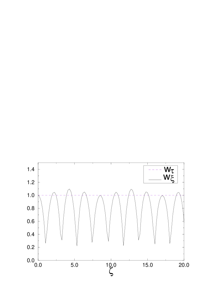
Figure 5: The results obtained using the variational method displaying the dependence of the temporal, $w_{\tau}$, and spatial, $w_{\xi}$, widths of the anomalous pulse (a) co-propagating with the normal pulse (b), for the following parammeters of the system: $\kappa_{1}=1.0,\sigma_{1}=1.0,\kappa_{2}=2.0,\sigma_{2}=0.0$.

a)
         
b)
         

Figure 6: The results obtained using the numerical simulations displaying the dependence of the temporal, $w_{\tau}$, and spatial, $w_{\xi}$, widths of the anomalous pulse (a) co-propagating with the normal pulse (b) for the following parammeters of the system: $\kappa_{1}=1.0,\sigma_{1}=1.0,\kappa_{2}=2.0,\sigma_{2}=0.0$.

6 Conclusions

In this paper properties of two pulses propagating simultaneously in different dispersion regimes, i.e. anomalous and normal, in a Kerr-type planar waveguide are considered. The propagation is described by two coupled NSEs. The interaction between pulses is assumed to be limited to cross-phase modulation. Four wave mixing is neglected, i.e. no energy transfer between pulses is taken into account. The accuracy of another assumption used in the analysis, the omitting of the difference of group velocities of the pulses, is discussed in appendix B. Our analysis is based on the variational method and numerical simulations.

First we studied the influence of the parameters of the pulse propagating in a normal dispersion regime on the threshold of catastrophic self-focusing of the pulse with an anomalous dispersion. We observed that catastrophic self-focusing of the pulse propagating in an anomalous dispersion regime can be arrested by the pulse propagating in a normal dispersion regime when the strength of nonlinearity is sufficiently large, $\kappa_{2}>\kappa_{Xlow}$ and the dispersion-to-diffraction ratio satisfies the relation: $|\sigma_{Xlow}(\kappa_{2})|<|\sigma_{2}|<|\sigma_{Xupp}(\kappa_{2})|$. In this notation $X\equiv V(X\equiv N)$ concerns the results obtained in the variational method (numerical simulations). We also investigated whether the nonlinear coupling between pulses can cause catastrophic self-focusing of the pulse propagating in a normal dispersion regime. The variational method indicates that when catastrophic self-focusing of the anomalous pulse occurs, the normal pulse can display, depending on the parameters of the system, two different characteristics: (i) both widths of the pulse initially decrease reaching a minimum on a certain distance of propagation and then they start to increase, (ii) the spatial width of the pulse vanishes to zero on a finite distance of propagation whereas the temporal width initially decreases reaching a minimum on a certain distance of propagation and then it increases. The occurence of catastrophic self-focusing of the normal pulse has not been observed in the numerical simulations. Therefore, we can conclude, based on the variational method and the numerical simulations, that catastrophic self-focusing of the anomalous pulse does not necessarily lead to catastrophic self-focusing of the normal pulse.

We found also, using the numerical simulations, that the presence of the pulse propagating in a normal dispersion regime can lead to spatio-temporal splitting of the pulse propagating in an anomalous dispersion regime. Recall that splitting of an anomalous pulse into several pulses does not occur when it propagates as a single pulse.

Finally, we considered the limiting case of vanishing dispersion of the pulse propagating in a normal dispersion regime with parameters of the pulses chosen in such a way that catastrophic self-focusing does not occur, i.e. that the conditions $\kappa_{1}<\kappa_{Vcat}=1+\sigma_{1}$ (in the variational method) and $\kappa_{1}<\kappa_{Ncat}\approx 0.885+\sigma_{1}$ (in the numerical simulations) are satisfied. The main motivation was to see whether such a configuration can lead to a stable self-trapped propagation of a pulse with anomalous dispersion. The positive answer was obtained within the variational method which confirms that neither spatio-temporal spreading nor catastrophic self-focusing of the anomalous pulse can develop thus giving rise to a self-trapped solution. Note that this kind of stabilization is similar to that which has been found earlier in media with saturation-type nonlinearity [12]. Although the existing data supports the existence of a self-trapped solution, conclusive results require labourious simulations at high values of the longitudinal variable $\zeta$ and are not yet available (work in progress).

Note, in conclusion, that the existence of a stable self-trapped solution could be useful, for example, in optical switching devices. The configuration of two simultaneously propagating pulses in a planar waveguide could also be of use in optical compression techniques.

7 Acknowledgements

The work was supported by the Polish Committee of Scientific Research (KBN, grant no 8T11F 007 14) and the Deutsche Akademische Austauschdienst (DAAD), to both of which I express my gratitude. I take the opportunity to express my thanks to Professor F. Lederer for his kind hospitality at the Institute of Solid State Physics and Theoretical Optics, Fredrich-Schiller-Universität Jena, Jena, Germany. The numerical calculations were partially done thanks to a fellowship at the Abdus Salam International Centre for Theoretical Physics, Trieste, Italy. I gratefully acknowledge the Director of the Centre Professor M. Virasoro, and Professor G. Denardo for their kind hospitality and helpful support. I also would like to thank the referees for constructive suggestions.

Appendix A

The notation in equations (1) and ($(2b)$a,b) is as follows [2]: $\zeta=z/{z_{DF1}}$ is the longitudinal coordinate normalized to the Fresnel diffraction length of the anomalous pulse, $\xi=x/{w_{1}}$ is the spatial transverse coordinate normalized to the initial spatial width of the anomalous pulse, $\tau=({t-\beta_{1}^{(1)}z})/{t_{1}}$ is the local time normalized to the initial temporal width of the anomalous pulse. The parameters $\sigma_{j}={z_{DF1}}/{z_{DSj}}$, $\mu={z_{DF1}}/{z_{DF2}}$, $r={\lambda_{1}}/{\lambda_{2}}={\omega_{2}}/{\omega_{1}}$ denote, respectively, the dispersion-to-diffraction ratio, the ratio of the Fresnel diffraction length of the anomalous pulse to the Fresnel diffraction length of the normal pulse and, finally, the ratio of the carrier frequency of the anomalous pulse to the carrier frequency of the normal pulse. $\Psi_{j}:=\sqrt{\kappa_{j}}{U_{j}(\zeta,\tau,\xi)}/{U_{j0}}$ denotes the normalized amplitude of the $j$-s pulse, where $U_{j}(\zeta,\tau,\xi)$ is the amplitude of the slowly varying envelope of the electric field, $U_{j0}:=U_{j}(0,0,0)$ is the dimensionless initial peak amplitude. The parameter $\kappa_{j}:=\left({z_{DFj}}/{z_{NLj}}\right)^{2}$ defined as the strength of nonlinearity of j-s pulse is proportional to the nonlinear part, $n_{2}$, of the refractive index of a medium, $n:=n_{0}+n_{2}|U_{j}|^{2}$, to the initial peak intensity, $|U_{j0}|^{2}$, and to the square of the spatial width of the pulse, $w^{2}_{\xi j}$. Note also that in the case of the (1+1)-dimensional NSE, i.e. when $\sigma_{j}=0$, the quantity $\sqrt{\kappa_{j}}$ can be interpreted as the order of a spatial soliton, so that a first-order soliton arises when $\kappa_{j}=1$ [61]. The dispersive terms are defined as follows: $\beta_{j}^{(0)}:=\beta^{(0)}(\omega_{j})={\omega_{j}}/c$ is the wavenumber, $\beta_{j}^{(1)}:={\partial\beta}/{\partial\omega}|_{\omega=\omega_{j}}=1/v_{gj}$ is the reverse group velocity, and $\beta_{j}^{(2)}:={\partial^{2}\beta}/{\partial\omega^{2}}|_{\omega=\omega_{j}}$ is the group velocity dispersion. The parameters $z_{DFj}:=\beta_{j}^{(0)}n_{0}(\omega_{j})w_{i}^{2}$, $z_{DSj}:={t_{j}^{2}}/{\beta_{j}^{(2)}}$, $z_{NLj}:=w_{j}\sqrt{{n_{0}}/{(2n_{2}|U_{0j}|^{2})}}$, $w_{j}$, $t_{j}$ denote, respectively, the Fresnel diffraction length, the dispersive length, the nonlinear length, the initial spatial width and the initial temporal width of the $j$-s pulse. In the above notation $j=1,2$, where the subscript $j=1$ ($j=2$) refers to the anomalous (normal) pulse.

Appendix B

Since we have assumed that pulses have different wavelengths and different group velocity dispersions, it is physically evident that they should also have different group velocities. Therefore, the assumption that the difference of the group velocities of the pulses vanishes is a simplification accepted in this paper and should be viewed as a first step of the analysis. When this difference does not vanish the pulses propagate with different velocities and the overlap between them decreases with the longitudinal variable. Therefore, the nonlinear coupling between them also decreases. In the limiting case of the difference of the group velocities of the pulses approaching infinity the coupling between pulses becomes zero and the problem of simultaneous propagation of two pulses reduces to the case when they propagate separately.

However, we believe that the inclusion of a small difference of group velocities of the pulses, which should be studied numerically, will not cause qualitative changes in the results of this paper, such as the possibility of an arresting of catastrophic self-focusing of the pulse propagating in an anomalous dispersion regime by the influence of the pulse propagating in a normal dispersion regime. The only difference we expect is a change of the values of the parameters, $\sigma_{Nlow},\sigma_{Nupp},$ $\kappa_{Nupp}$, which describe the threshold of catastrophic self-focusing for fixed values of $\sigma_{1}$ and $\kappa_{1}$. These quantitative changes would be proportional to the value of the difference of the group velocities of the pulses.

References

- [1] Y. Silberberg, Opt. Lett. 15, 1282 (1990).
- [2] A. T. Ryan and G. P. Agrawal, Opt. Lett. 20, 306 (1995).
- [3] M. Desaix, D. Anderson, and M. Lisak, J.Opt.Soc.Am. B. 8, 2082 (1991).
- [4] V. E. Zakharov and A. B. Shabat, Zh. Exp. Teor. Fiz. 61, 118 (1971).
- [5] G. Fibich, Phys. Rev. Lett. 76, 4356 (1996).
- [6] S. N. Vlasov, V. A. Petrishchev, and V. I. Talanov, Izv. Vuz Radiofiz. 14, 1353 (1971).
- [7] J. J. Rasmussen and K. Rypdal, Physica Scrypta 33, 481 (1986).
- [8] X. D. Cao, G. P. Agrawal, and C. J. McKinstrie, Phys. Rev. A 49, 4085 (1994).
- [9] J. T. Manassah, P. L. Baldeck, and R. Alfano, Opt. Lett. 13, 1090 (1988).
- [10] P. Chernev and V. Petrov, Opt. Comm. 87, 28 (1992).
- [11] M. Pietrzyk, Opt. and Q.E. 29, 579 (1997).
- [12] M. Karlsson, Phys. Rev. A 46, 2726 (1992).
- [13] D. Suter and T. Blasbberg, Phhys. Rev A 47, 256 (1993).
- [14] A. L. Dyshko, V. N. Lugovi, and A. M. Prokhorov, Sov. Phys. JETP 34, 1235 (1972).
- [15] E. Yablonovitch and B. Bloembergen, Phys. Rev. Lett. 29, 907 (1972).
- [16] S. Henz and J. Hermann, Phys. Rev. E 53, 4092 (1996).
- [17] V. I. Karpman, Phys. Rev. E 53, R1336 (1996).
- [18] S. Blair and K. Wagner, Opt. and Q.E. 30, 697 (1998).
- [19] N. Akhmediev, A. Ankiewicz, and J. M. Soto-Crespo, Opt. Lett. 18, 411 (1993).
- [20] G. Fibich and G. C. Papanicolaou, Opt. Lett. 22, 1379 (1997).
- [21] I. Gurwich, J. Phys. D 30, 2183 (1997).
- [22] M. D. Feit and J. J. A. Fleck, J. Opt. Soc. Am. B 5, 633 (1988).
- [23] A. P. Sheppard and M. Healtermand, Opt. Lett. 23, 1820 (1998).
- [24] F. H. Berkshire and J. D. Gibbon, Stud. Applied Math. 69, 229 (1983).
- [25] A. G. Litvak, T. A. Petrova, A. M. Sergeev, and A. D. Yunakovskii, Sov. J. Plasma Phys. 9, 287 (1993).
- [26] M. Pietrzyk, PhD thesis, Warsaw 1998 (in Polish, unpublished) .
- [27] B. Gross and J. T. Manassah, Opt. Comm. 126, 269 (1996).
- [28] D. Burak and R. Binder, in Proc. Quantum Electronics and Laser Science Conference (OSA, USA, 1996).
- [29] J. E. Rothenberg, Opt. Lett. 17, 1340 (1992).
- [30] P. Chernev and V. Petrov, Opt. Lett. 17, 172 (1992).
- [31] G. G. Luther, J. V. Moloney, A. C. Newell, and E. M. Wright, Opt. Lett. 19, 862 (1994).
- [32] J. E. Rothenberg, Opt. Lett. 17, 583 (1992).
- [33] M. Trippenbach and Y. B. Band, Phys. Rev. A 56, 4242 (1997).
- [34] A. A. Zozulya, S. A. Diddams, A. G. VanEugen, and T. S. Clement, Phys. Rev. Lett. 82, 1430 (1999).
- [35] A. A. Zozulya and S. A. Diddams, Opt. Express 4, 336 (1999).
- [36] J. K. Ranka and A. L. Gaeta, Opt. Lett. 23, 534 (1998).
- [37] J. K. Ranka, R. W. Schirmer, and A. L. Gaeta, Phys. Rev. Lett. 77, 3783 (1996).
- [38] S. A. Diddams, H. K. Eaton, A. A. Zozulya, and T. S. Clement, Opt. Lett. 23, 379 (1998).
- [39] C. J. McKinstrie and D. A. Russell, Phys. Rev. Lett. 61, 2929 (1988).
- [40] L. Berge, Phys. Rev. E 58, 6606 (1998).
- [41] A. S. Desyatnikov and A. I. Maimistov, J. Exp. Theor. Phys. 86, 1101 (1998).
- [42] O. Bang, L. Berge, and J. J. Rasmussen, Phys. Rev. E 59, 4600 (1999).
- [43] G. P. Agrawal, Phys. Rev. Lett. 64, 2487 (1990).
- [44] K. Konno and H. Suzuki, Phys. Scripta 20, 382 (1979).
- [45] R. McLeod, K. Wagner, and S. Blair, Phys. Rev. A 52, 3254 (1995).
- [46] F. Vidal and T. W. Johnston, Phys. Rev. Lett. 77, 1282 (1996).
- [47] S. Gatz and J. Herrmann, J. Opt. Soc. Am. B 14, 1795 (1997).
- [48] V. Skarka, V. I. Berezhiani, and R. Miklaszewski, Phys. Rev. E 56, 1080 (1997).
- [49] M. Segev, B. Crosignani, and A. Yariv, Phys. Rev. Lett. 68, 923 (1992).
- [50] M. F. Shih and M. Segev, Phys. Rev. Lett. 78, 2551 (1997).
- [51] B. A. Malomed et al., Phys. Rev. E 56, 4725 (1997).
- [52] L. Berge, V. K. Mezentsev, J. J. Rasmussen, and J. Wyller, Phys. Rev. A 52, R28 (1995).
- [53] K. Hayata and M. Koshiba, Phys. Rev. Lett. 71, 3275 (1993).
- [54] D. Mihalache, D. Mazilu, L. C. Crasovan, and L. Torner, Opt. Comm. 137, 113 (1997).
- [55] P. Agin and G. I. Stegeman, JOSA B 14, 3162 (1997).
- [56] W. E. Torruellas et al., Phys. Rev. Lett. 74, 5036 (1995).
- [57] X. Liu, L. J. Qian, and F. W. Wise, Phys. Rev. Lett. 82, 4631 (1999).
- [58] L. Berge, O. Bang, J. J. Rasmussen, and V. K. Mezentsev, Phys. Rev. E 55, 3555 (1997).
- [59] S. Darmanyan, I. Relke, and F. Lederer, Phys. Rev. E 55, 7662 (1997).
- [60] D. Anderson and M. Bonnedal, Phys. Fluids 22, 105 (1979).
- [61] G. P. Agrawal, ”Nonlinear Fiber Optics” (Academic Press, London, 1989).
- [62] D. Anderson, M. Lisak, and T. Reicher, J. Opt. Soc. Am. B 5, 207 (1988).
- [63] W. H. Press, S. A. Teukolsky, W. T. Vetterling, and B. P. Flannery, ”Numerical Recipes in Fortran” (Cambridge University Press, Cambridge, 1992).
- [64] F. Cornolti, M. Lucchesi, and B. Zambon, Opt. Comm 75, 129 (1990).
- [65] M. Desaix, D. Anderson, and M. Lisak, Phys. Rev. E 50, 2253 (1994).
- [66] L. Berge et al., J. Opt. Soc. Am. B 13, 1879 (1996).
- [67] D. Burak and W. Nasalski, J. Tech. Phys. 36, 199 (1995).
- [68] D. Anderson, Phys. Rev. A 27, 3135 (1983).
- [69] D. Burak, Opt. Appl. 21, 3 (1991).