Origin of Multikinks in Dispersive Nonlinear Systems

Abstract

We develop the first analytical theory of multikinks for strongly dispersive nonlinear systems, considering the examples of the weakly discrete sine-Gordon model and the generalized Frenkel-Kontorova model with a piecewise parabolic potential. We reveal that there are no $2\pi$-kinks for this model, but there exist discrete sets of $2\pi N$-kinks for all $N>1$. We also show their bifurcation structure in driven damped systems.

Non-equilibrium dynamics of many physical systems can be characterized by the creation and motion of topological excitations or defects. In particular, when a nonlinear system possesses a degeneracy of its ground state, such excitations are kinks, the simplest and probably most studied nonlinear modes. The concept of kinks is vital for many physical problems such as dislocation and mass transport in solids, charge-density waves, commensurable-incommensurable phase transitions, conductivity, tribology, Josephson transmission lines, etc [1].

In application to problems in solid state physics, the kink’s motion is strongly affected by the inherent lattice discreteness. Earlier numerical simulations [2] of the kink’s motion in a lattice described by the discrete sine-Gordon (SG) equation, also known as the Frenkel-Kontorova (FK) model [1], demonstrated a number of interesting features not observed in the dynamics of solitons of integrable (both continuous and discrete) models. In particular, Peyrard and Kruskal [2] found that a single kink becomes unstable when it moves in a discrete lattice at sufficiently large velocity, whereas two (or more) kinks are stable and propagate as multikinks. The former effect is associated with resonant interaction between a kink and radiation [3], and resonances are even observed experimentally [4]. In contrast, the latter phenomenon, i.e. the formation of multikinks, “… has no clear analytical explanation yet” (see [1], p. 25).

Recently, different physical systems have been studied numerically where multikinks are found to play an important role. For example, multikinks are responsible for a mobility hysteresis in a damped driven commensurable chain of atoms [5]. In arrays of Josephson junctions, instabilities of fast kinks lead to the generation of bunched fluxon states also described by multikink modes [6].

The main purpose of this paper is to provide the first step towards an analytical theory of multikinks in strongly dispersive nonlinear nonintegrable systems, including the analysis of the existence and codimension of $N-$kink states. In particular, we consider a weakly discrete SG model and demonstrate the existence of a finite number of multikinks due to a higher-order dispersion. We also find analytical solutions for multikinks and describe the effect of an external field and damping on their existence and qualitative features.

We consider the dynamics of a commensurable chain of atoms in a periodic substrate potential. In a normalized form, the equations of motion for the atomic displacements $u_{n}$ can be written as

$\displaystyle\ddot{u}_{n}=V_{\rm int}^{\prime}(a_{0}+u_{n+1}-u_{n})-V^{\prime}_{\rm int}(a_{0}+u_{n}-u_{n-1})-W^{\prime}_{\rm sub}(u_{n}),$

where $V_{\rm int}(u)$ is an effective interaction potential with the equilibrium distance $a_{0}$, and $W_{\rm sub}(u)$ is a substrate potential with period $a$. For small anharmonicity, i.e. when $|u_{n+1}-u_{n}|\ll a_{0}$, the potential $V_{\rm int}(u)$ can be expanded into a Taylor series to yield (see details in Ref. [1]): $\ddot{u}_{n}-g(u_{n+1}+u_{n-1}-2u_{n})+W_{\rm sub}^{\prime}(u_{n})=0$, where $g\equiv V_{\rm int}^{\prime\prime}(a_{0})$. In the quasi-continuum limit, taking into account a higher-order dispersion, we obtain the normalized equation

$$u_{tt}-u_{xx}-\beta u_{xxxx}+W_{\rm sub}^{\prime}(u)=0,$$ (1)

where $W(u)$ has rescaled period $2\pi$ and, for harmonic interaction, $\beta=a^{2}/12$.

Equation (1) takes into account the effect of lattice discreteness through a fourth-order dispersion term, and for $\beta=0$ and $W_{\rm sub}^{\prime}(u)=\sin\,u$, it transforms into the well-known exactly integrable SG equation that has an analytical solution for a single $2\pi$-kink moving with velocity $v$, $u=4\tan^{-1}\{\exp[(x-vt)/\sqrt{1-v^{2}}]\}$. Similar kinks exist for a rather general topology of the substrate potential $W_{\rm sub}(u)$ [1]. However, our aim in this paper is to study a new class of localised solutions of Eq. (1) for $\beta\neq 0$ in the form of $2\pi N$-multikinks for $N>1$.

First, following the original study of Peyrard and Kruskal [2], we consider the harmonic substrate potential

$$W_{\rm sub}(u)=1-\cos\,u\,.$$ (2)

We look for kink-type localised solutions of Eq. (1) that move with velocity $v$ $(v^{2}<1)$, i.e. we assume $u(z)=u(x-vt)$. Linearizing Eq. (1) and taking $u(z)\sim e^{\lambda z}$, we find eigenvalues $\lambda$ of the form,

$\displaystyle\lambda^{2}=\frac{1}{2\beta}[(v^{2}-1)\pm\sqrt{(1-v^{2})^{2}+4\beta}],$

so that for $\beta>0$ there always exist two real and two purely imaginary eigenvalues. Thus, the origin $u=0$ is a saddle-centre point and hence kinks, which are homoclinic solutions to $u=0$ (mod $2\pi$), should occur for isolated values of $v$ for fixed $\beta$ (see Refs. [7, 8]). That is they are of codimension one. Moreover, this codimension is only true if the solutions are themselves reversible, that is invariant under one of the transformations:

$$\begin{array}[]{l}{\ R_{1}:\quad u(\mbox{mod}\>2\pi)\to-u(\mbox{mod}\>2\pi),\;u^{\prime\prime}\to-u^{\prime\prime},\quad t\to-t,}\\[9.0pt] {\displaystyle R_{2}:\quad u^{\prime}\to-u^{\prime},\quad u^{\prime\prime\prime}\to-u^{\prime\prime\prime},\quad t\to-t,}\end{array}$$

where prime stands for differentiation with respect to $z$.

FIG. 1.: The four $4\pi$-kink solutions of Eq. (1) with $W_{\rm sub}^{\prime}(u)=\sin\,u$ propagating at the given velocities.

To find all solutions of this type, first we fix $\beta=1/12$, which corresponds to $a=1$. Then, we perform numerical shooting on the ordinary differential equation for $u(z)$ using a well-established Newton-type method for homoclinic/heteroclinic trajectories in reversible systems (see [9]). The first result is that there exists no $2\pi$-kink solution at all, except in the artificial limit $v^{2}\to-\infty$ (see comment below). Instead, we find a discrete family of $4\pi$-kinks; specifically there exist only four such solutions at four different values of $v$. The first solution has an analytical form [10]

$$u(z)=8\tan^{-1}\exp\left\{(3\beta)^{1/4}z\right\},$$ (3)

where $v^{2}=1-2\sqrt{\beta/3}$, i.e. for our choice of $\beta$, $v_{4\pi}^{(1)}=\sqrt{2/3}$. Other values are: $v_{4\pi}^{(2)}=0.59498\ldots$, $v_{4\pi}^{(3)}=0.42373\ldots$, and $v_{4\pi}^{(4)}=0.21109\ldots$. All these solutions are presented in Fig. 1. We may regard this discrete family as part of an infinite sequence of bound-states of two $2\pi$-kinks that converges to the limit of infinite separation at a value of $v^{2}<0$. Actually the key parameter is $\mu=1-v^{2}$, and further numerical evidence reveals that the bound states converge to $\mu=\infty$ at which value a $2\pi$-kink exists only formally.

In addition to the $4\pi$-kinks, numerics further reveals $v$-values at which $2\pi N$-kinks occur for all $N>2$. Figure 2 shows several examples of $6\pi$- and $8\pi$-kinks. According to a dynamical systems theory result [7], on the existence of bound states of homoclinic solutions to saddle-centre equilibria in reversible Hamiltonian systems, again thinking of the $4\pi$-kinks as bound states of $2\pi$-kinks, one should expect to see precisely two $6\pi$-kinks for each $4\pi$-kink. These would occur at $v_{6\pi}^{(i),\pm}$ satisfying $v_{6\pi}^{(i)-}<v_{4\pi}^{(i)}<v_{6\pi}^{(i)+}$; all eight of which are depicted in Fig. 2(a). Moreover, there would be two infinite sequences of $8\pi$-kinks at $v_{8\pi}^{(i,j)\pm}$ such that $v_{8\pi}^{(i,j)-}\to v_{4\pi}^{(i)}$ from below as $j\to\infty$ and $v_{8\pi}^{(i,j)+}\to v_{4\pi}^{(i)}$ from above. Our numerical simulations have revealed precisely this structure of all multikink families.

FIG. 2.: Examples of (a) $6\pi$- and (b) $8\pi$-kinks of Eq. (1) with the potential (2) at given velocities.

FIG. 3.: Two-parameter continuation of $4\pi$-kink solutions for the model (1) with the harmonic nonlinearity (2).

Finally, it appears that the above structure is largely independent of $\beta$. Figure 3 shows the results of continuation (using the method for homo/heteroclinic orbits in the boundary-value software AUTO [11]) of the four $4\pi$-kinks in the $(v,1/\sqrt{\beta})$ plane. These curves are almost identical to those obtained numerically in Ref. [2] for the discrete SG equation. Note that no curve passes through $v=1$, they only reach there asymptotically as $\beta\to 0$. In the process the slope of each kink at its midpoint steepens, so that the solution becomes singular in the limit.

It is important that the above numerical results may be verified by the construction of exact solutions in closed form when the substrate potential is approximated by a piecewise parabolic potential that generates in Eq. (1) the effective force, $W_{\rm sub}^{\prime}(u)=$

$$\left\{\begin{array}[]{l}{u-2n\pi\>:(2n-1)\pi+\pi/2<u<2n\pi+\pi/2},\\ {(2n+1)\pi-u\>:2n\pi+\pi/2<u<(2n+1)\pi+\pi/2}.\end{array}\right.$$

For simplicity we fix $\beta=1/12$ and then look for kinks moving with velocity $v$ ($\mu=1-v^{2}$), by solving the piecewise-linear equation for $u(z)$. This defines a four-dimensional dynamical system in the phase space $(u,u^{\prime},u^{\prime\prime},u^{\prime\prime\prime})\in(-\pi/2,3\pi/2]\times{\bf R}^{3}$. The phase space is separated into two distinct domains:

$\displaystyle\mbox{\text@underline{Region 1}}:|u|<\pi/2,\quad\mbox{\text@underline{Region 2}}:\pi/2<u<3\pi/2.$

$4\pi$-kinks can be constructed by first noticing that, in order to be of codimension-one (i.e. occur at isolated $v$-values), they should be reversible under the transformation $R_{1}$ above. Since we can always translate by multiples of $2\pi$, we look for solutions which satisfy, for some unknown $z_{2}$, the conditions: $u(-\infty)\rightarrow 0$, $u(z_{2})=2\pi$, and $u^{\prime\prime}(z_{2})=0$, so that $u(z)$ is in Region 1 for all $z<0$, in Region 2 for $0<z<z_{1}$, for some unknown $z_{1}<z_{2}$, and is in Region 1 again for all $z_{1}<z<z_{2}$.

The boundary condition can be satisfied by noticing that such solutions at $z=0$ (the first point of transition between Regions 1 and 2) satisfy $u(0)=\pi/2$, $u^{\prime}(0)=\lambda\pi/2$, $u^{\prime\prime}(0)=\lambda^{2}\pi/2$, and $u^{\prime\prime\prime}(0)=\lambda^{3}\pi/2$, where $\lambda^{2}=6(\sqrt{\mu^{2}+2/3\pi}-\mu)$ is the unique real positive eigenvalue of the linear system in Region 1. Hence the asymptotic boundary condition at $z=-\infty$ in Region 1 becomes an initial condition at $z=0$ for $u$ in Region 2. The general solutions in Regions 1 and 2 are:

$\displaystyle u_{1}(z)=A_{1}e^{\lambda z}+B_{1}e^{\lambda z}+C_{1}\cos(\omega z)+D_{1}\sin(\omega z)$

and, providing $\mu>\mu_{\rm min}:=\sqrt{2/3\pi}$,

$\displaystyle u_{2}(z)=A_{2}\cos(\omega_{1}z+B_{2})+C_{2}\cos(\omega_{2}z+D_{2})$

where $\omega^{2}=6(\sqrt{\mu^{2}+2/3\pi}+\mu)$ and $\omega_{1,2}^{2}=6(\mu\pm\sqrt{\mu^{2}-2/3\pi})$, $A_{j}$, $B_{j}$, $C_{j}$, and $D_{j}$ are unknown coefficients. Therefore, we can explicitly solve for the coefficients to find $u_{2}(z)$ in closed form. This expression defines an implicit equation for $z_{1}$; $u_{2}(z_{1})=3\pi/2$. The value of $u_{2}(z_{1})$ and its derivatives then defines initial conditions at $z=z_{1}$, hence determining the constants $A_{1}$, $B_{1}$, $C_{1}$, and $D_{1}$. This in turn defines $z_{2}$ implicitly as $u_{1}(z_{2})=2\pi$. To have a $4\pi$-kink we additionally require $u_{1}^{\prime\prime}(z_{2})=0$, and so should only expect to find zeros of this final quantity by varying $v$. Hence we can define a ‘test function’ for $4\pi$-kinks $K(v;z_{1},z_{2}):=u_{2}^{\prime\prime}(z_{2})$. Using the above construction, this $K$ can be written in closed form in terms of $v$, $z_{1}$, and $z_{2}$. The unknown transition points $z_{1,2}$ are the solution to given transcendental equations, in each case only the first solution of which has meaning.

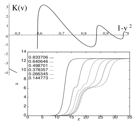
FIG. 4.: The function $K(v)$ for multikinks of Eq. (1) with piecewise parabolic potential. Inset: the corresponding $4\pi$-kinks and their associated $v$-values.

Figure 4 shows a graph of $K$ as a function of $\mu=1-v^{2}\in(\mu_{\rm min},1)$, which has been computed using MAPLE with the implicit equations solved for their smallest positive solutions. The five zeros of $K$ correspond to $4\pi$-kinks, graphs of which are shown in the insert to the figure. These zeros occur for $v=0.64064609$, 0.49870155, 0.37835717, 0.26634472, 0.14477294. It is also possible to construct solutions for $\mu<\mu_{\rm min}$ in a analogous manner, but with the solution in Region 2 replaced by one corresponding to complex eigenvalues. This gives the additional solution for $v=0.833706$.

In this way, we find analytically a finite set of $v$-values giving $4\pi$-kinks for the piecewise parabolic potential model, having qualitatively the same structure as the solutions found numerically for the sinusoidal nonlinearity (2). One could go on to construct $2\pi N$-kinks for $N>2$, but the calculations presented already serve to corroborate the earlier numerical results.

To complete the analysis of the kinks, we would like to mention that the short-wavelength instability of the nonstationary continuous model (1) due to the term $u_{xxxx}$ can be easily removed by introducing an equivalent higher-order dispersion via a mixed derivative term [1, 12].

To analyse the robustness of multikinks in realistic physical systems, we add to the right-hand side of Eq. (1) the driven damped term $F-\delta u_{t}$, where $F$ is an external DC force and $\delta$ is a damping coefficient (see, e.g., [5]). Importantly, for each of the kinks so far found, it is possible to use numerical continuation to trace curves that lie on sheets in the parameter space $(v,\delta,F)$ corresponding to the existence of multikinks. For example, taking the explicit $4\pi$-kink solution given by Eq. (3), a curve was computed at $\beta=1/12$ in the $(F,v\delta)$-plane with fixed $|v|=\sqrt{2/3}$, reaching a maximum with respect to $\delta$ at $|v|\delta=0.069326$. Taking the fixed value $|v|\delta=0.05$ from this curve the locus of kinks in the $(v,F)$-plane can then be traced out, as depicted in Fig. 5.

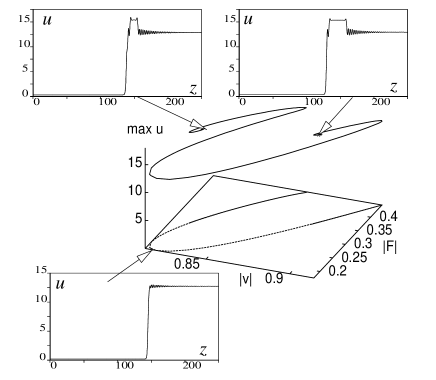
FIG. 5.: The kink’s velocity $v<0$ and maximum amplitude against external force $F>0$ for the simplest $4\pi$ kink with $v\delta=0.05$. Note that each limb of the curve spirals back on itself. The insets illustrate example solutions on the locus.

Three interesting features can be noted from this curve. First, all kinks have developed oscillations around the equilibrium close to $u=4\pi$. This is because, for $\delta>0$, the corresponding equation for travelling waves is no longer Hamiltonian or reversible, and the linearization around the asymptotic value $u_{\star}=\sin^{-1}F$ now has three stable eigenvalues, two of which have non-zero imaginary part. These oscillations may be regarded as radiation that travels at the kink’s velocity, as was earlier observed in direct numerical simulations [6]. Second, $v$ and $F$ have opposite sign for these results. When $F$ and $v$ have the same sign, only kinks with non-decaying oscillations in the tails can be found. Third, note that the computed curve ends at a point where a transition takes place involving a heteroclinic connection with $u\approx 5\pi$. This suggests that $\pi$-kinks are possible for sufficiently large $F$.

Finally, we mention that the case $\beta<0$ in Eq. (1) can also occur in generalised nonlinear lattices provided we take into account the next-neighbor interactions, e.g. due to the so-called helicoidal terms in nonlinear models of DNA dynamics [13]. In this case, the analysis is much simpler and, similar to the nonlocal SG equations [14], leads to the continuous families of multikinks parameterized by $v$. From the mathematical point of view, for $\beta<0$ the origin changes from a saddle-center to a saddle-focus, and rigorous variational principles [15] give families of stable $2\pi N$-kinks for all $N>1$.

In conclusion, we have developed the first analytical theory of multikinks in strongly dispersive nonlinear systems, considering the important examples of the generalized FK model with the sinusoidal and piecewise parabolic potentials. We have revealed, numerically and analytically, the existence of discrete sets of $2\pi N$-kinks. We believe that general features of multikinks and the physical mechanism for their formation are similar in many other strongly dispersive nonlinear models.

Yuri Kivshar thanks O.M. Braun, A.S. Kovalev, B. Malomed, M. Peyrard, and A. Ustinov for useful discussions. Alan Champneys is indebted to the Optical Sciences Centre for hospitality and to the UK EPSRC with whom he holds an advanced fellowship.

REFERENCES

- [1] See, e.g., O.M. Braun and Yu.S. Kivshar, Phys. Rep. 306, 1 (1998); and references therein.
- [2] M. Peyrard and M. Kruskal, Physica D 14, 88 (1984).
- [3] See, e.g., A.V. Ustinov, M. Cirillo, and B.A. Malomed, Phys. Rev. B 47, 8357 (1993).
- [4] H.S.J. van der Zant, T.P. Orlando, S. Watanabe, and S.H. Strogatz, Phys. Rev. Lett. 74, 174 (1995).
- [5] O.M. Braun, T. Dauxois, M.V. Paliy, and M. Peyrard, Phys. Rev. Lett. 78, 1295 (1997); O.M. Braun, A.R. Bishop, and J. Röder, Phys. Rev. Lett. 79, 3692 (1997).
- [6] A.V. Ustinov, B.A. Malomed, and S. Sakai, Phys. Rev. B 57, 11691 (1998).
- [7] A. Mielke, P. Holmes, and O. O’Reilly, J. Dyn. Diff. Eqns. 4, 95 (1998).
- [8] A.R. Champneys, Physica D 112, 158 (1998).
- [9] A.R. Champneys, and A. Spence, Adv. Comp. Math. 1, 81 (1993).
- [10] M.M. Bogdan and A.M. Kosevich, In Nonlinear Coherent Structures in Physics and Biology, Eqs. K.H. Spatschek and F.G. Mertens (Plenum, New York, 1994), p. 373.
- [11] E.J. Doedel, A.R. Champneys, T.R. Fairgrieve, Yu.A. Kuznetsov, B Sanstede, and W. Wang, AUTO97 Continuation and Bifurcation Software for Ordinary Differential Equations, 1997. Available by anonymous ftp from ftp.cs.concordia.ca, directory pub/doedel/auto.
- [12] P. Rosenau, Phys. Lett. A 118, 222 (1986).
- [13] G. Gaeta, C. Reiss, M. Peyrard, and T. Dauxois, Rivista Nuovo Cim. 17, 1 (1994).
- [14] G.L. Alfimov and V.G. Korolev, Phys. Lett. A 246, 429 (1998).
- [15] W.D. Kalies and R.A.C.M. van der Vorst, J. Diff. Eqns. 131, 209 (1996); W.D. Kalies, J. Kwapisz and R.A.C.M. van der Vorst, Comm. Math. Phys. 193, 337 (1998).