Planform selection in two-layer Benard-Marangoni convection

Abstract

Bénard-Marangoni convection in a system of two superimposed liquids is investigated theoretically. Extending previous studies the complete hydrodynamics of both layers is treated and buoyancy is consistently taken into account. The planform selection problem between rolls, squares and hexagons is investigated by explicitly calculating the coefficients of an appropriate amplitude equation from the parameters of the fluids. The results are compared with recent experiments on two-layer systems in which squares at onset have been reported.

PACS: 47.20.-k, 47.20.Dr, 47.20.Bp, 47.54.+r, 68.10.-m

I Introduction

The hexagonal convection cells discovered by Bénard in his famous experiments on thin oil layers heated from below [1] have become the trademark of pattern formation in hydrodynamic systems driven slightly out of equilibrium (see e.g. [2]). The hundred years of research devoted to this system have revealed several important insights but also witnessed several misconceptions. Rayleigh’s original theoretical description [3] focusing on buoyancy-driven convection, though indicating a possible instability mechanism, failed to produce a threshold compatible with experiment. Not until forty years later was it realized that the temperature dependence of the surface tension is the crucial driving force in thin layers [4]. The corresponding linear stability analysis [5] gave stability thresholds consistent with the experimental findings, moreover, a subsequent weakly non-linear analysis [6, 7] produced theoretical support for a sub-critical transition to a hexagonal flow pattern [8].

Quite naturally the first theoretical investigations were performed using simplified models of the experimental situation. The initial assumption of a flat surface of the liquid was soon relaxed by Scriven and Sternling [9] and Smith [10] who were able to show that surface deflections give rise to an additional instability appearing at very long wavelengths. It was only very recently that this instability was unambiguously demonstrated in an experiment [11] where it manifests itself as a distortion of the layer thickness with a characteristic length which is of the order of the lateral extension of the fluid layer. Being observable only in very shallow liquid layers, the instability usually results in the formation of dry spots.

Another common simplification is the restriction of the instability mechanism to either buoyancy or thermocapillarity [12, 13, 18], although there seem to be rather few experiments [14, 8, 11] which have been performed in parameter regions with the ratio between the Rayleigh and the Marangoni number being sufficiently different from unity. Also, most investigations focussed on a single layer model in which a lower liquid layer is in contact with a gaseous upper layer and only the hydrodynamics of the liquid are treated. The convection in the gas layer is neglected and the heat exchange between the layers is often modeled in a phenomenological way using a Biot number, see e.g. [15]. Even if a genuine two layer model is considered the viscous stresses and the pressure variations in the gaseous layer are neglected in order to keep the analysis simple [13].

On the other hand it has been known for some time [12, 16] that a system of two superimposed liquids displays a much richer behaviour than the single layer models. In particular the Marangoni instability can be induced by heating from above such that buoyancy and thermocapillarity compete rather than enhance each other, a situation which in single layer systems can only be realized using the rare case of liquids with anomalous thermocapillary effect in which the surface tension increases with increasing temperature [17]. Many additional features such as oscillatory instabilities [18] or transitions from up- to down-hexagons may be found in systems with two liquid layers. The rich variety of phenomena occurring in the theoretical analysis of the two-layer liquid systems results in part from their huge parameter space. A single layer system is characterized by just three dimensionless parameters; namely, the Rayleigh number, the Marangoni number and the Prandtl number. The latter is irrelevant in the linear analysis and the first two are both proportional to the temperature difference across the layer. Two layer systems on the other hand may easily need ten or more dimensionless parameters for a complete specification. These numbers include the ratios of the hydrodynamic parameters of the participating liquids.

For a long time Marangoni convection in two-liquid-layer systems was an interesting theoretical problem but too difficult to handle experimentally. Already Zeren and Reynolds [12] tried to experimentally realize the instability by heating from above which came out of their theoretical analysis but failed. Very recently, however, experiments where performed in which the Marangoni instability in 1-2 mm thick superimposed layers of immiscible liquids was observed [21, 22]. In particular an instability by heating from above and square patterns at the onset were reported.

In the present paper we will investigate theoretically Bénard-Marangoni convection in a system of two liquid layers. Building on the linear stability theory developed in [23] we perform a weakly non-linear analysis in order to solve the planform selection problem slightly above the linear stability threshold. To this end the competition between rolls, squares and hexagons will be discussed. Only perfect patterns will be considered leaving the question of weakly modulated patterns for future investigations. We will consistently include buoyancy effects and treat the full hydrodynamics of both liquids, generalizing in this way various previous treatments [6, 13, 15, 24, 25, 26]. However, we will assume a flat interface between the two liquids. As will become clear below, interface distortions are crucial for the long wavelength instability resulting in dry spots but can be safely neglected when dealing with the finite wavelength instability resulting in cellular patterns.

The paper is organized as follows. In section 2 the basic equations are collected and transformed into a form suitable for the weakly non-linear analysis. Then the perturbation scheme is set up and the necessary computational steps are listed. Section 3 deals with the first order of the perturbation theory which is nothing but the linear stability analysis. In section 4 the main steps of the nonlinear analysis are outlined. The solution of the second order problem is relegated to appendix C and the solvability condition in third order is then formulated to derive the desired amplitude equation characterizing the planform selection problem. Section 5 discusses the results obtained for some experimentally relevant combinations of liquids. Finally section 6 contains a discussion of the results together with a comparison with experimental findings.

II Basic equations

We investigate a system of two layers of immiscible and incompressible liquids of thickness $h^{(i)}$ with densities $\rho^{(i)}$, kinematic viscosities $\nu^{(i)}$, coefficients of volume expansion $\alpha^{(i)}$, heat diffusivities $\chi^{(i)}$, and thermal conductivities $\kappa^{(i)}$ where the superscript $i=1$ (2) denotes the lower (upper) fluid (see fig.1). The system is bounded in the vertical direction by two solid, perfectly heat conducting walls with fixed temperatures $T^{b}$ and $T^{t}$ and is infinite in the horizontal directions. The interface between the two fluids is assumed to be flat and to lie in the $x$-$y$-plane of the coordinate system.

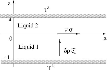
FIG. 1.: Sketch of the system under consideration. One liquid layer is superposed on another between two horizontally infinite, perfectly heat conducting plates. The interface between the liquids is assumed to be flat. Convection arises due to buoyancy and the temperature dependence of the surface tension.

The hydrodynamics of the two liquids will be described within the Boussinesq approximation, i.e. we assume that all parameters are independent of the temperature, except for the densities $\rho^{(i)}$ and the interface tension $\sigma$. More precisely we use $\rho^{(i)}(T)=\rho^{(i)}(T^{b})(1-\alpha^{(i)}(T-T^{b}))$ and $\nabla_{\perp}\sigma=d\sigma/dT\,\nabla_{\perp}T$ with constant $\alpha^{(i)}$ and $d\sigma/dT$. Neglecting heat production due to viscosity, the basic equations describing the system are the continuity equations

$$\nabla\boldsymbol{v}^{(i)}=0\quad,$$ (1)

the Navier-Stokes equations

$$\partial_{t}\boldsymbol{v}^{(i)}+(\boldsymbol{v}^{(i)}\nabla)\boldsymbol{v}^{(i)}=-\frac{1}{\rho^{(i)}}\nabla p^{(i)}-g(1-\alpha^{(i)}(T^{(i)}-T^{b}))\boldsymbol{e}_{z}+\nu^{(i)}\Delta\boldsymbol{v}^{(i)}\quad,$$ (2)

and the equations of heat conduction

$$\partial_{t}T^{(i)}+(\boldsymbol{v}^{(i)}\nabla)T^{(i)}=\chi^{(i)}\Delta T^{(i)}\quad.$$ (3)

Here $\boldsymbol{e}_{z}$ denotes the unit vector in the vertical direction and $g$ is the acceleration due to gravity.

These equations are completed by the boundary conditions

$$\boldsymbol{v}^{(1)}=0\quad,\quad T^{(1)}=T^{b}\quad\text{at}\quad z=-h^{(1)}\quad,$$ (4)

and

$$\boldsymbol{v}^{(2)}=0\quad,\quad T^{(2)}=T^{t}\quad\text{at}\quad z=h^{(2)}\quad,$$ (5)

at bottom and top respectively and

$$\boldsymbol{v}^{(1)}=\boldsymbol{v}^{(2)}\quad,\quad T^{(1)}=T^{(2)}\quad,\quad\kappa^{(1)}\partial_{z}T^{(1)}=\kappa^{(2)}\partial_{z}T^{(2)}$$ (6)

$$\left[(\sigma^{(2)}-\sigma^{(1)})\boldsymbol{e}_{z}\right]_{\perp}=-\frac{d\sigma}{dT}\nabla_{\perp}T\quad,\quad\boldsymbol{v}^{(1)}_{z} =\boldsymbol{v}^{(2)}_{z}=0\quad,\qquad\text{at}\quad z=0\quad,$$ (7)

expressing the continuity of the velocities, temperatures and heat fluxes respectively as well as the balance of tangential stresses at the interface. The $\sigma^{(i)}$ denote the stress tensors in the liquids and the subscript $\perp$ describes the projection to the $x$-$y$-plane. In accordance with our assumption of a flat interface between the liquids the condition for the continuity of the normal stress at the interface is replaced by the requirement that the perpendicular components of the flow velocities must vanish. This is expressed by the last equation in (6) .

Introducing $h^{(1)}$, $(h^{(1)})^{2}/\chi^{(1)}$, $\chi^{(1)}/h^{(1)}$ and $\rho^{(1)}\nu^{(1)}\chi^{(1)}/(h^{(1)})^{2}$ as units for length, time, velocity, and pressure respectively we find for the velocities $\boldsymbol{v}=(u,v,w)\,(\boldsymbol{V}=(U,V,W))$ and the appropriately normalized deviations $\theta\,(\Theta)$ of the temperatures from their static profiles in the lower (upper) liquid the equations:

$$\frac{1}{Pr}(\partial_{t}\boldsymbol{v}+(\boldsymbol{v}\nabla)\boldsymbol{v}) =-\nabla\tilde{p}+R\,\theta\,\boldsymbol{e}_{z}+\Delta\boldsymbol{v}$$ (8)

$$\partial_{t}\theta+(\boldsymbol{v}\nabla)\theta =w+\Delta\,\theta$$ (9)

$$\frac{1}{Pr}(\partial_{t}\boldsymbol{V}+(\boldsymbol{V}\nabla)\boldsymbol{V}) =-\nabla\tilde{P}+\alpha\,R\,\Theta\,\boldsymbol{e}_{z}+\nu\Delta\boldsymbol{V}$$ (10)

$$\partial_{t}\Theta+(\boldsymbol{V}\nabla)\Theta =\frac{1}{\kappa}\,W+\chi\Delta\Theta\quad,$$ (11)

where the pressure fields $\tilde{p}$ and $\tilde{P}$ in the lower and the upper liquid differ from $p^{(1)}$ and $p^{(2)}$ respectively only by trivial contributions stemming from the buoyancy terms. The boundary conditions acquire the form

$$\boldsymbol{v}=0\quad,\quad\theta=0\quad\text{at}\quad z=-1\quad,$$ (12)

$$\boldsymbol{V}=0\quad,\quad\Theta=0\quad\text{at}\quad z=a\quad,$$ (13)

and

$$\boldsymbol{v}_{\perp}=\boldsymbol{V}_{\perp}\,,\,w =W=0\,,\,\theta=\Theta\,,\,\partial_{z}\theta=\kappa\partial_{z}\Theta\,,\,\partial^{2}_{z}w-\eta\partial^{2}_{z}W=M\Delta_{\perp}\theta\,,\quad\text{at}\,z=0\,,$$ (14)

where in the last equation the continuity equation was used. Moreover the following parameters have been introduced:

$$a=\frac{h^{(2)}}{h^{(1)}}\;,\;\alpha=\frac{\alpha^{(2)}}{\alpha^{(1)}}\;,\;\nu=\frac{\nu^{(2)}}{\nu^{(1)}}\;,\;\eta=\nu\frac{\rho^{(2)}}{\rho^{(1)}}\;,\;\kappa=\frac{\kappa^{(2)}}{\kappa^{(1)}}\;,\;\chi=\frac{\chi^{(2)}}{\chi^{(1)}}\;,$$ (15)

as well as the Prandtl-number $Pr=\nu^{(1)}/\chi^{(1)}$, the Rayleigh-number

$$R=\frac{\alpha^{(1)}g(h^{(1)})^{3}}{\nu^{(1)}\chi^{(1)}}\frac{\kappa}{a+\kappa}(T^{b}-T^{t})\quad,$$ (16)

and the Marangoni-number

$$M=-\frac{d\sigma}{dT}\frac{h^{(1)}}{\nu^{(1)}\rho^{(1)}\chi^{(1)}}\frac{\kappa}{a+\kappa}(T^{b}-T^{t})\quad.$$ (17)

For the Rayleigh- and Marangoni-number we have chosen the standard expressions corresponding to the lower liquid. The respective numbers for the upper liquid are then given by

$$R^{(2)}=\frac{\alpha a^{4}}{\nu\chi\kappa}R\quad\text{and}\quad M^{(2)}=\frac{a^{2}}{\chi\eta\kappa}M$$ (18)

respectively.

The ratio between the Rayleigh and Marangoni numbers determines whether the occurring instability is predominantly driven by buoyancy or by surface tension. Experimentally both parameters are varied simultaneously since they are both proportional to the temperature difference $T^{b}-T^{t}$. We will therefore replace $R$ by $cM$ with the temperature independent constant

$$c=\frac{R}{M}=-\frac{\alpha^{(1)}g(h^{(1)})^{2}}{d\sigma/dT}$$ (19)

specifying the experimental setup. In this way both buoyancy and surface tension are included in a consistent way. We assume that $d\sigma/dT<0$ as is the case for most systems of two liquids such that $c>0$. Note that both the situation of heating from below and heating from above are described with the latter case corresponding to $M<0$.

The set of equations may be simplified by standard manipulations. Taking twice the curl of the Navier-Stokes equations, using the continuity equations, and projecting onto $\boldsymbol{e}_{z}$ we get the following basic set of equations for the $z$-components of the velocities and the temperature fields:

$$\Delta^{2}w+cM\Delta_{\perp}\theta =\frac{1}{Pr}\left[\partial_{t}\Delta w-\partial_{z}(\nabla_{\perp}(\boldsymbol{v}\nabla)\boldsymbol{v}_{\perp})+\Delta_{\perp}(\boldsymbol{v}\nabla)w\right]$$ (20)

$$w+\Delta\theta =\partial_{t}\theta+(\boldsymbol{v}\nabla)\theta$$ (21)

$$\nu\Delta^{2}W+\alpha cM\Delta_{\perp}\Theta =\frac{1}{Pr}\left[\partial_{t}\Delta W-\partial_{z}(\nabla_{\perp}(\boldsymbol{V}\nabla)\boldsymbol{V}_{\perp})+\Delta_{\perp}(\boldsymbol{V}\nabla)W\right]$$ (22)

$$\frac{1}{\kappa}W+\chi\Delta\Theta =\partial_{t}\Theta+(\boldsymbol{V}\nabla)\Theta$$ (23)

together with the boundary conditions

$$w =\partial_{z}w=\theta=0\quad\text{at}\quad z=-1$$ (24)

$$w =W=0\,,\,\partial_{z}w=\partial_{z}W\,,\,\theta=\Theta\,,\,\partial_{z}\theta=\kappa\partial_{z}\Theta\,,\,\partial^{2}_{z}w-\eta\partial^{2}_{z}W=M\Delta_{\perp}\theta\quad\text{at}\quad z=0$$ (25)

$$W =\partial_{z}W=\Theta=0\quad\text{at}\quad z=a$$ (26)

In order to investigate the planform selection problem we will derive third order amplitude equations for the slow time variation of the amplitudes of different unstable modes. Similar to the case of the Rayleigh-Bénard instability [2] the no-slip boundary conditions at top and bottom suppress the vertical vorticity, i.e. $(\nabla\times\boldsymbol{v})\boldsymbol{e}_{z}=(\nabla\times\boldsymbol{V})\boldsymbol{e}_{z}=0$, and therefore we do not expect problems due to a coupling to a slowly varying mean flow [28] up to this order. From the solution of (20)-(23) we hence obtain $w,\theta,W$ and $\Theta$. Using the continuity equations and the absence of vertical vorticity allows to determine $u,v$ and $U,V$ and finally the pressure fields follow from the Navier-Stokes equations.

It is convenient to write the above equations in the form

$$L\varphi=\cal{T}(\varphi)+\cal{N}(\varphi,\varphi)$$ (27)

with the state vector

$$\varphi=\begin{pmatrix}w\\ \theta\\ W\\ \Theta\end{pmatrix}\quad,$$ (28)

and the linear operator $L$ defined by

$$L=\begin{pmatrix}\Delta^{2}&cM\Delta_{\perp}&0&0\\ 1&\Delta&0&0\\ 0&0&\nu\Delta^{2}&\alpha cM\Delta_{\perp}\\ 0&0&\frac{1}{\kappa}&\chi\Delta\\ \end{pmatrix}\quad,$$ (29)

and the boundary conditions (24)-(26). $\cal{T}(\varphi)$ denotes the time dependent terms and $\cal{N}(\varphi,\varphi)$ describes the quadratic nonlinearity in (20)-(23). We will solve (27) perturbatively using the ansätze

$$\varphi =\varepsilon\varphi_{0}+\varepsilon^{2}\varphi_{1}+\varepsilon^{3}\varphi_{2}+\dots$$ (30)

$$M =M_{c}+\varepsilon M_{1}+\varepsilon^{2}M_{2}+\dots$$ (31)

$$\partial_{t} =i\omega\qquad\quad\;\;+\varepsilon^{2}\partial_{\tau}+\dots$$ (32)

with a small parameter $\varepsilon$. In the case of a static instability we have $\omega=0$ whereas for an oscillatory instability $\omega\neq 0$ gives the frequency of oscillation of the unstable mode. Using the perturbation expansion specified above we consider a situation slightly above the threshold $M_{c}$ of the linear instability, where the amplitude of the unstable modes can still be considered to be small. Plugging (30)-(32) into (27), taking into account that (31) implies an expansion

$$L=L_{0}+\varepsilon L_{1}+\varepsilon^{2}L_{2}+\dots$$ (33)

for the linear operator and matching powers of $\varepsilon$ the non-linear problem transforms into a sequence of linear equations of the form

$$L_{0}\varphi_{0} =0$$ (34)

$$L_{0}\varphi_{1} =-L_{1}\varphi_{0}+{\cal N}(\varphi_{0},\varphi_{0})$$ (35)

$$L_{0}\varphi_{2} =-L_{2}\varphi_{0}-L_{1}\varphi_{1}+{\cal T}(\varphi_{0})+{\cal N}(\varphi_{1},\varphi_{0})+{\cal N}(\varphi_{0},\varphi_{1})\quad.$$ (36)

The first line is just the linear stability problem. The condition for non-trivial solutions $\varphi_{0}$ of this equation makes $L_{0}$ singular and yields the critical value $M_{c}$ of the bifurcation parameter $M$. From the translation invariance in the $x$-$y$-plane we know that $\varphi_{0}$ is of the form

$$\varphi_{0}=\varphi_{0}(z)\exp(i\boldsymbol{k}\boldsymbol{r}-i\omega t)$$ (37)

where $\boldsymbol{r}=(x,y)$ and $\boldsymbol{k}=(k_{x},k_{y})$ are two-dimensional vectors. There is a critical value $M_{c}(k)$ of the bifurcation parameter for all values of $|\boldsymbol{k}|=k$ and minimizing $M_{c}(k)$ in $k$ gives the wavenumber $k_{c}$ of the first unstable mode together with the critical Marangoni number $M_{c}=M_{c}(k_{c})$.

The remaining equations in the hierarchy starting with (35) all involve the very same singular operator $L_{0}$ but are inhomogeneous. Consequently the perturbation expansion makes sense only if the inhomogeneities are perpendicular to the zero eigenfunction of the adjoint operator $L^{+}_{0}$ of $L_{0}$.

FIG. 2.: Relative orientation of the two-dimensional wave vectors appearing in the ansatz (38). The two triads $\boldsymbol{k}_{1},\boldsymbol{k}_{2},\boldsymbol{k}_{3}$ and $\boldsymbol{k}_{4},\boldsymbol{k}_{5},\boldsymbol{k}_{6}$ of wave vectors with $\boldsymbol{k}_{5}$ perpendicular to $\boldsymbol{k}_{1}$ allow to describe rolls as well as squares and hexagons by different values for the amplitudes $A_{n}$ in (38).

In order to address the planform selection problem within the perturbation approach sketched above the form of $\varphi_{0}$ must be sufficiently general and in particular must include the different planforms observed in the experiment. We will discuss the planform selection problem only for the case of the static instability leaving the investigation of the oscillatory instability to future work. It is then sufficient to use for $\varphi_{0}$ the form

$$\varphi_{0}=\varphi_{0}(z)\left[\sum_{n=1}^{6}A_{n}(\tau)e^{i\boldsymbol{k}_{n}\boldsymbol{r}}+\text{c.c.}\right]$$ (38)

with the six two-dimensional vectors $\boldsymbol{k}_{n}$ obeying $|\boldsymbol{k}_{n}|=k_{c}$ and $\boldsymbol{k}_{1}+\boldsymbol{k}_{2}+\boldsymbol{k}_{3}=0$, $\boldsymbol{k}_{4}+\boldsymbol{k}_{5}+\boldsymbol{k}_{6}=0$, as well as $\boldsymbol{k}_{1}\boldsymbol{k}_{5}=0$ (see fig.2). Depending on the values of the amplitudes $A_{n}$ this form describes rolls (e.g. $A_{1}=A,A_{n}=0$ for all $n>1$), squares (e.g. $A_{1}=A_{5}=A,A_{n}=0$ else) and hexagons (e.g. $A_{1}=A_{2}=A_{3}=A$, $A_{n}=0$ for $n>3$).

Using this form we find from the solvability conditions of (35) and (36) an equation describing the time evolution of the scaled amplitudes $\tilde{A_{n}}=\varepsilon A_{n}$. As is well known [2] the general form of this amplitude equation already follows from the symmetries of the problem. For the present situation it is given by

$$\partial_{t}\tilde{A}_{1}=\epsilon\tilde{A}_{1}+\gamma\tilde{A}_{2}^{*}\tilde{A}_{3}^{*}-\left[|\tilde{A}_{1}|^{2}+g_{h}(|\tilde{A}_{2}|^{2}+|\tilde{A}_{3}|^{2})+g_{t}(|\tilde{A}_{4}|^{2}+|\tilde{A}_{6}|^{2})+g_{n}|\tilde{A}_{5}|^{2}\right]\tilde{A}_{1}$$ (39)

with the super-criticality parameter

$$\epsilon=\frac{M-M_{c}}{M_{c}}\quad.$$ (40)

Similar equations for the other amplitudes follow from permutation and complex conjugation. The terms included in these equations are the only ones up to third order which are invariant under the transformation $A_{n}\mapsto A_{n}\exp(i\boldsymbol{k}_{n}\boldsymbol{r}_{0})$ corresponding to a translation by $\boldsymbol{r}_{0}$ in the $x$-$y$-plane. Moreover due to the isotropy in the $x$-$y$-plane the coupling coefficients between the different terms in (38) may only depend on the angle between the corresponding wave vectors.

A well known linear stability analysis of the various fix points of (39) yields the stability regions of the different planforms as functions of the parameters $\epsilon,\gamma,g_{h},g_{t},g_{n}$ [27]. The remaining problem is hence to use the perturbation expansion described above to express these coefficients of the amplitude equation in terms of the hydrodynamic parameters of the problem. To this end the following well-known program has to be carried through:

• Calculate $M_{c}(k)$ from the linear problem and determine $k_{c}=\text{argmin}\,M_{c}(k)$ and $M_{c}=M_{c}(k_{c})$.

• Determine the adjoint operator $L^{+}_{0}$ of $L_{0}$ and its zero eigenfunction $\bar{\varphi}_{0}$.

• Calculate the inhomogeneity of the $O(\varepsilon^{2})$-equation (35) and apply the solvability condition to this order.

• Solve the $O(\varepsilon^{2})$-equation (35) to determine $\varphi_{1}$.

• Calculate the inhomogeneity of the $O(\varepsilon^{3})$-equation (36) (only terms proportional to $\exp{i(\boldsymbol{k}_{1}\boldsymbol{r})}$ are necessary)

• Combine the solvability conditions at order $O(\varepsilon^{2})$ and $O(\varepsilon^{3})$ to derive (39) and extract the expressions for the parameters $\gamma,g_{h},g_{t},g_{n}$.

III The linear problem

We first solve the $O(\varepsilon)$ problem (34), which is equivalent to the linear stability analysis. Putting $\varphi_{0}=\varphi_{0}(z)\exp(i\boldsymbol{k}\boldsymbol{r}-i\omega t)$ and using the ansätze

$$w_{0}(z),\theta_{0}(z) \sim\exp(\lambda z)\qquad \qquad W_{0}(z),\Theta_{0}(z) \sim\exp(\Lambda z)$$ (41)

we find

$$(\lambda^{2}-k_{c}^{2})(\lambda^{2}-k_{c}^{2}+\frac{i\omega}{Pr})(\lambda^{2}-k_{c}^{2}+i\omega) =-cMk_{c}^{2}\quad \quad(\Lambda^{2}-k_{c}^{2})(\Lambda^{2}-k_{c}^{2}+\frac{i\omega}{\nu Pr})(\Lambda^{2}-k_{c}^{2}\frac{i\omega}{\chi}) =-\frac{\alpha}{\nu\kappa\chi}cMk_{c}^{2}\quad.$$ (42)

We therefore obtain six different values for $\lambda_{i}$ and $\Lambda_{i}$. It is convenient to define $\lambda_{i}=\Lambda_{i-6}$ for $i=7,\dots,12$ and to write

$$w_{0}(z) =\sum_{i=1}^{6}w_{0i}\,e^{\lambda_{i}z}\qquad \qquad\theta_{0}(z) =-\sum_{i=1}^{6}\frac{w_{0i}}{\lambda_{i}^{2}-k_{c}^{2}+i\omega}\,e^{\lambda_{i}z}$$ (43)

$$W_{0}(z) =\sum_{i=7}^{12}w_{0i}\,e^{\lambda_{i}z}\qquad \qquad\Theta_{0}(z) =-\frac{1}{\kappa\chi}\sum_{i=7}^{12}\frac{w_{0i}}{\lambda_{i}^{2}-k_{c}^{2}+\frac{i\omega}{\chi}}\,e^{\lambda_{i}z}$$ (44)

The boundary conditions (24)-(26) give then rise to a homogeneous system of linear equations for the 12 unknowns $w_{0i}$. In order to get a non-trivial solution the determinant of the coefficient matrix ${\cal A}$ must vanish. The conditions for the real and the imaginary part of det${\cal A}$ yield the desired functions $M_{c}(k;\text{par})$ and $\omega_{c}(k,\text{par})$ where $\text{par}=(a,\alpha,\kappa,\chi,\nu,\eta,c,Pr)$ stands for the vector of parameters in the problem.

FIG. 3.: Dispersion relation $M_{c}(k)$ as resulting from the linear stability analysis for the hydrodynamic parameters of setup 2 listed in appendix A. The system shows an instability when heated from below as well as one when heated from above.

A typical result for a static instability is shown in fig.3 displaying the dispersion curve resulting from the numerical analysis of det${\cal A}=0$ for $\omega=0$ using the parameters of setup 2 listed in appendix A. As can be seen from the figure in this system one may have an instability by heating from below ($M>0$) as well as when heating from above ($M<0$). In fig.4 the results of the present approach for the setups 1 and 5 of appendix A are compared with those resulting from the full linear stability analysis including surface deflections as considered in [23]. As is clearly seen in the region of the pattern forming instability $k\cong 1...3.5$ the two curves are almost identical with differences showing up only for small wave numbers $k\ll 1$. Within the linear theory the surface deflections for unstable modes corresponding to the planform selection problem may therefore safely be neglected and we expect that this is also a good approximation for the weakly non-linear regime.

FIG. 4.: Comparison of the dispersion relation $M_{c}(k)$ as resulting from the present analysis assuming a flat interface between the liquids (thin full lines) with the results of the complete linear analysis of [23] including surface deflections (dashed lines). The lower right curves are for setup 1, the others for setup 5 specified in appendix A.

Having obtained the dispersion relation we calculate $k_{c}$ by minimizing $M_{c}(k)$ and determine the critical Marangoni and Rayleigh numbers of both fluids as well as the temperature difference across both layers at the instability. The results for the setups under consideration are summarized in the upper part of table 1.

From all the parameters of the system the depth ratio $a$ is the only one which may be easily varied in the experiments. For the parameters of setup 3 and a total depth of 4.5 mm we have calculated the critical Marangoni number and the critical wave number modulus as a function of the thickness $h^{(1)}$ of the bottom layer restricting ourselves to the case of heating from below but including the possibility of an oscillatory instability. The results are displayed in fig.5. For values of $h^{(1)}$ between 1.5 and 2.5 an oscillatory instability precedes the static one which would occur at unusually large Marangoni numbers only. A similar oscillatory instability was also found for a two-layer system in which the Marangoni effect was neglected and pure buoyancy-driven convection was considered, and an intuitive interpretation as a periodic change between viscous and thermal coupling of the flow fields at the interface was given [18]. The oscillatory instability was also detected in the experiment using setup 3 with $h^{(1)}\cong 1.8$mm and the experimental values for the critical Marangoni number and the wavelength of the oscillatory mode are in good agreement with the theory [22].

FIG. 5.: Critical Marangoni number for heating from below a system with parameters as specified in setup 3 of appendix A and total depth 4.5 mm as a function of the bottom layer thickness $h^{(1)}$. Note that both $M$ and $k$ are scaled with $h^{(1)}$ (cf. (15) and (17)).

Knowing the critical value of $M$ we can now also determine the coefficients of the eigenvector corresponding to the zero eigenvalue. This fixes the functions $w_{0}(z),\theta_{0}(z),W_{0}(z)$ and $\Theta_{0}(z)$ up to an overall constant and completes the determination of $\varphi_{0}$.

Finally we have to consider the adjoint problem and to calculate its zero eigenfunction $\bar{\varphi}_{0}$ where we again restrict ourselves to the stationary instability. The adjoint operator $L^{+}$ is determined in appendix B. The calculation of its eigenfunction to the eigenvalue zero is very similar to the determination of $\varphi_{0}$ described above. We find that it is of the form $\bar{\varphi_{0}}\exp(i\boldsymbol{k}_{n}\boldsymbol{r})$ where the components of $\bar{\varphi_{0}}$ may be written as

$$\bar{w}_{0}(z) =\sum_{i=1}^{6}\bar{w}_{0i}\,e^{\lambda_{i}z}\qquad \qquad\bar{\theta}_{0}(z) =cMk_{c}^{2}\sum_{i=1}^{6}\frac{\bar{w}_{0i}}{\lambda_{i}^{2}-k_{c}^{2}}\,e^{\lambda_{i}z}$$ (45)

$$\bar{W}_{0}(z) =\sum_{i=7}^{12}\bar{w}_{0i}\,e^{\lambda_{i}z}\qquad \qquad\bar{\Theta}_{0}(z) =\frac{\alpha cMk_{c}^{2}}{\chi}\sum_{i=7}^{12}\frac{\bar{w}_{0i}}{\lambda_{i}^{2}-k_{c}^{2}}\,e^{\lambda_{i}z}$$ (46)

with the same parameters $\lambda_{i}$ as determined by (42) with $\omega=0$. The boundary conditions give again rise to a $12\times 12$ system of linear homogeneous equations for the coefficients $\bar{w}_{0i}$. As before the condition for a non-trivial solution is a vanishing determinant of the corresponding matrix. Note, however, that there is now no parameter to adjust! The deviation of the smallest eigenvalue of the matrix found in the numerical calculation from zero gives therefore a valuable hint on the accuracy of the numerical procedure employed.

IV The nonlinear analysis

The solution of the planform selection problem requires the treatment of the nonlinear interaction between different unstable modes. To include nonlinear terms up to the third order in the amplitudes $A_{n}$ introduced in (38) we have first to solve (35). The general procedure is standard, some intermediate steps are sketched in appendix C. Using this solution we are in the position to calculate the terms appearing on the right hand side of (36). We do not have to solve this equation, but only need to know the solvability condition at this order. Due to the $x$-$y$-integrals in (B9) and the $\boldsymbol{r}$-dependence of $\bar{\varphi_{0}}$ only terms proportional to $\exp(\pm i\boldsymbol{k}_{n}\boldsymbol{r})$ give rise to non-trivial contributions to the solvability condition. In fact it is sufficient to focus on terms proportional to $\exp(i\boldsymbol{k}_{1}\boldsymbol{r})$ since these finally give rise to an amplitude equation of the form (39) for $A_{1}$. Equivalent equations for the other amplitudes of the ansatz (38) follow then from permutation and complex conjugation.

In order to collect the relevant terms we first realize that there are contributions

$$A_{1}\,e^{i\boldsymbol{k}_{1}\boldsymbol{r}}\begin{pmatrix}c\,M_{2}\,k_{c}^{2}\theta_{0}\\ 0\\ \alpha c\,M_{2}\,k_{c}^{2}\Theta_{0}\\ 0\\ -M_{2}\,k_{c}^{2}\theta_{0}|_{z=0}\end{pmatrix}\quad,\quad A_{2}^{*}A_{3}^{*}\,e^{i\boldsymbol{k}_{1}\boldsymbol{r}}\begin{pmatrix}c\,M_{1}\,k_{c}^{2}\theta_{1}\\ 0\\ \alpha c\,M_{1}\,k_{c}^{2}\Theta_{1}\\ 0\\ -M_{1}\,k_{c}^{2}\theta_{1}|_{z=0}\end{pmatrix}\quad,\quad\partial_{\tau}A_{1}\,e^{i\boldsymbol{k}_{1}\boldsymbol{r}}\begin{pmatrix}\frac{1}{Pr}(w_{0}^{\prime\prime}-k_{c}^{2}w_{0})\\ \theta_{0}\\ \frac{1}{Pr}(W_{0}^{\prime\prime}-k_{c}^{2}W_{0})\\ \Theta_{0}\\ 0\end{pmatrix}\quad,$$ (47)

originating from the terms $-L_{2}\varphi_{0}$, $-L_{1}\varphi_{1}$, and ${\cal T}(\varphi_{0})$ respectively in (36). Here $\theta_{1}$ and $\Theta_{1}$ denote the solutions obtained in the last section for the resonant term.

The contributions proportional to $\exp(i\boldsymbol{k}_{1}\boldsymbol{r})$ from the last two terms in (36) arise from combinations between $\varphi_{0}\sim\exp(i\boldsymbol{q}\boldsymbol{r})$ and $\varphi_{1}\sim\exp(i\boldsymbol{p}\boldsymbol{r})$ with $\boldsymbol{q}+\boldsymbol{p}=\boldsymbol{k}_{1}$. From the continuity equation, $\nabla\boldsymbol{v}=0$, and the absence of vertical vorticity, $(\nabla\times\boldsymbol{v})\boldsymbol{e}_{z}=0$, we find

$$\boldsymbol{v}_{0\perp}=e^{i\boldsymbol{q}\boldsymbol{r}}\,\frac{i\boldsymbol{q}}{\boldsymbol{q}^{2}}\,\partial_{z}w_{0}\qquad,\qquad\boldsymbol{v}_{1\perp}=e^{i\boldsymbol{p}\boldsymbol{r}}\,\frac{i\boldsymbol{p}}{\boldsymbol{p}^{2}}\,\partial_{z}w_{1}\quad,$$ (48)

which gives rise to

$$-\partial_{z}(\nabla_{\perp}(\boldsymbol{v}_{0}\nabla)\boldsymbol{v}_{1\perp})+\Delta_{\perp}(\boldsymbol{v}_{0}\nabla)w_{1}-\partial_{z}(\nabla_{\perp}(\boldsymbol{v}_{1}\nabla)\boldsymbol{v}_{0\perp})+\Delta_{\perp}(\boldsymbol{v}_{1}\nabla)w_{0}=\\ e^{i\boldsymbol{k}_{1}\boldsymbol{r}}\!\!\left[\frac{\boldsymbol{k}_{1}\boldsymbol{q}}{\boldsymbol{q}^{2}}w_{0}^{\prime\prime\prime}w_{1}\!+\!(\frac{\boldsymbol{k}_{1}\boldsymbol{q}}{\boldsymbol{q}^{2}}-\frac{\boldsymbol{q}\boldsymbol{p}}{\boldsymbol{q}^{2}\boldsymbol{p}^{2}}k_{c}^{2})w_{0}^{\prime\prime}w_{1}^{\prime}\!+\!(\frac{\boldsymbol{k}_{1}\boldsymbol{p}}{\boldsymbol{p}^{2}}-\frac{\boldsymbol{q}\boldsymbol{p}}{\boldsymbol{q}^{2}\boldsymbol{p}^{2}}k_{c}^{2})w_{0}^{\prime}w_{1}^{\prime\prime}\!+\!\frac{\boldsymbol{k}_{1}\boldsymbol{p}}{\boldsymbol{p}^{2}}w_{0}w_{1}^{\prime\prime\prime}+k_{c}^{2}\left((\frac{\boldsymbol{q}\boldsymbol{p}}{\boldsymbol{q}^{2}}-1)\,w_{0}^{\prime}w_{1}\!+\!(\frac{\boldsymbol{q}\boldsymbol{p}}{\boldsymbol{p}^{2}}-1)\,w_{0}w_{1}^{\prime}\right)\right]$$ (49)

and

$$(\boldsymbol{v}_{0}\nabla)\theta_{1}+(\boldsymbol{v}_{1}\nabla)\theta_{0}=e^{i\boldsymbol{k}_{1}\boldsymbol{r}}\left[-\frac{\boldsymbol{q}\boldsymbol{p}}{\boldsymbol{q}^{2}}\,w_{0}^{\prime}\theta_{1}-\frac{\boldsymbol{q}\boldsymbol{p}}{\boldsymbol{p}^{2}}\,w_{1}^{\prime}\theta_{0}+w_{0}\theta_{1}^{\prime}+w_{1}\theta_{0}^{\prime}\right]\quad.$$ (50)

With the help of these relations it is now easy to determine the remaining terms proportional to $\exp(i\boldsymbol{k}_{1}\boldsymbol{r})$ from all the possible combinations for $\boldsymbol{q}$ and $\boldsymbol{p}$ and the corresponding results for $\varphi_{1}$ calculated in appendix C.

Using the scalar product (B9) and the result for $\bar{\varphi_{0}}$, the solvability condition at order $O(\varepsilon^{3})$ can be formulated. It contains a term proportional to $M_{1}A_{2}^{*}A_{3}^{*}$ which by eliminating $M_{1}$ using the solvability condition (C11) at order $O(\varepsilon^{2})$ is transformed into terms proportional to $|A_{2}|^{2}A_{1}$ and $|A_{3}|^{2}A_{1}$. We then multiply the solvability condition at order $O(\varepsilon^{2})$ by $\varepsilon^{2}$ and the one at order $O(\varepsilon^{3})$ by $\varepsilon^{3}$ and add them together. Observing $\varepsilon M_{1}+\varepsilon^{2}M_{2}=M-M_{c}$, returning to the original time by using $\varepsilon^{2}\partial_{\tau}=\partial_{t}$ and introducing the scaled amplitudes $\tilde{A}_{n}=\varepsilon A_{n}$ we eventually end up with an amplitude equation of the form (39) with explicit expressions for the parameters $\gamma,g_{h},g_{t}$ and $g_{n}$.

V Results

The expressions for $\gamma,g_{h},g_{t}$ and $g_{n}$ are rather long and will not be displayed. Moreover, due to the large number of parameters in the two liquid system it is more appropriate to analyze some experimentally relevant parameter combinations rather than to display cross sections along some direction of the parameter space. For the five experimental setups specified in appendix A the results of the non-linear analysis are summarized in the lower part of table 1.

In order to finally address the planform selection problem we note that from the linear stability analysis of the roll, square and hexagon solutions of the amplitude equation (39) it is well known [27, 15] that:

• rolls are stable if $g_{h}>1$, $g_{t}>1$, $g_{n}>1$, and $\epsilon>\frac{\gamma^{2}}{(1-g_{h})^{2}}$,

• squares are stable if $1+g_{n}<g_{h}+g_{t}$, $|g_{n}|<1$, and $\epsilon>\frac{\gamma^{2}(1+g_{n})}{(1+g_{n}-g_{h}-g_{t})^{2}}$,

• hexagons are stable if $1+2g_{h}>0$, $\epsilon>\epsilon_{h}=-\frac{\gamma^{2}}{4(1+2g_{h})}$, either $g_{h}<1$ or $\epsilon<\epsilon_{htr}=\frac{\gamma^{2}(2+g_{h})}{(1-g_{h})^{2}}$, and either $1+2g_{h}<g_{n}+2g_{t}$ or $\epsilon<\epsilon_{hts}=\frac{\gamma^{2}(g_{n}+2g_{t})}{(1+2g_{h}-g_{n}-2g_{t})^{2}}$.

In addition to the special values of $\epsilon$ defined in the last point above we have also included in table 1 the amplitude $A_{h}$ of the pattern at onset. The hexagon pattern appears through a backward bifurcation which strictly speaking invalidates our perturbation ansatz (30). However, the interval of sub-critical hexagons as well as the amplitude of the pattern at onset are for all investigated setups rather small such that the ansatz is still a good approximation for what really happens.

Except for setup 3 when heated from below we always find $g_{n}<1$ excluding the possibility of stable rolls within the framework of our weakly non-linear analysis. For all setups we get $1+2g_{h}>0$ which implies that for hexagons the cubic term is able to stabilize the linear instability. Moreover for all setups $g_{h}>1$ and $1+2g_{h}>g_{n}+2g_{t}$ implying that the values of $\epsilon_{htr}$ and $\epsilon_{hts}$ give the stability border for hexagons. Being the result of an expansion in the amplitude of the unstable modes the numerical values of $\epsilon_{htr}$ and $\epsilon_{hts}$ are only reliable if they are not too large. If these values are hopelessly outside the validity of our perturbation approach they are not displayed in table 1. In all other cases we find $\epsilon_{htr}>\epsilon_{hts}$ for setups with $g_{n}<1$ in accordance with the fact that rolls are then unstable to squares. The value of $\epsilon_{hts}$ is always positive which means that exactly at onset our analysis always predicts hexagons as the stable planform and excludes squares. However, in the cases where $\epsilon_{hts}$ is rather small (e.g. setup 4 when heated from below) hexagons get very quickly unstable to squares when passing the stability threshold.

The sign of $\gamma$ is related to the detailed convection pattern of the hexagon planform. For $\gamma>0$ the hexagons in the lower fluid are up-hexagons (liquid rises in the center) and the one in the upper layer are down-hexagons. For $\gamma<0$ the situation is reversed. We do not know of experimental results concerning this feature for the two liquid Marangoni problem.
      setup 1 setup 2 setup 3 setup 4 setup 5 $\Delta T$ 0.415 4.032 -3.945 1.523 -0.256 0.859 -18.957 1.718 $k_{c}$ 2.495 2.745 0.714 4.3416 1.0328 2.377 0.861 1.901 $M$ 453 1919 -1878 1978 -333 869 -19188 379 $R$ 676 654 -640 669 -113 733 -16168 45 $M^{(2)}$ 24.1 614 -601 12107 -2036 149 -3284 777 $R^{(2)}$ 4.88 592 -579 8145 -1370 49 -1091 143 $\gamma$ 0.406 0.367 -0.559 -0.7478 -0.5428 0.423 -0.507 0.430 $g_{h}$ 1.225 1.196 1.411 1.57 1.36 1.188 1.417 1.377 $g_{t}$ 1.442 1.480 1.501 1.021 1.529 1.164 1.273 1.551 $g_{n}$ 0.030 0.419 0.075 1.594 -0.027 -0.355 -0.050 0.628 $\epsilon_{h}$ -0.012 -0.010 -0.020 -0.034 -0.020 -0.013 -0.017 -0.012 $A_{h}$ 0.118 0.108 0.1462 0.180 0.146 0.125 0.132 0.114 $\epsilon_{htr}$ - - 6.30 6.12 7.50 - 5.04 4.38 $\epsilon_{hts}$ 1.670 - 1.734 7.922 1.848 0.180 0.358 -

Table 1: Results for the critical temperature difference $\Delta T$ over both liquids ($\Delta T>0$ for heating from below, $\Delta T<0$ for heating from above), the critical wavenumber $k_{c}$, the Marangoni and Rayleigh numbers of both liquids at onset, the parameters of the amplitude equation (39), the sub-critical threshold $\epsilon_{h}$ for the hexagonal pattern, its amplitude $A_{h}$ at onset, and the values $\epsilon_{htr}$ and $\epsilon_{hts}$ at which the hexagon pattern gets unstable towards the formation of rolls and squares respectively. If the numerical values of $\epsilon_{htr}$ and $\epsilon_{hts}$ obtained are larger than 10 they are meaningless as result of a perturbation expansion in $\epsilon$ and are therefore not displayed.

For the parameters of setup 3 and a total depth of 4.5 mm we have again scanned the dependence of the results of the non-linear analysis on the thickness of the bottom layer for the case of heating from below. Fig.6 shows the coefficients of the amplitude equation (39) as functions of $h^{(1)}$. The most apparent feature is the strong sensitivity of the coefficients on variations of the depth ratio. In experiments the depth must therefore be controlled very accurately in order to allow sensible comparison with the theory. The system under consideration shows a transition from up to down hexagons when varying the depth ratio as can be seen from the change of the sign of $\gamma$.

FIG. 6.: The parameters $g_{h}$ (full), $g_{t}$ (dashed), $g_{n}$ (dotted) and $\gamma$ (dashed-dotted) of the amplitude equation (39) as functions of the thickness $h^{(1)}$ of the bottom layer for setup 3 with a total layer depth of 4.5 mm and heating from below. For 1.5 mm$\lesssim h^{(1)}\lesssim 2.5$ mm the oscillatory instability precedes the static one.

Finally in fig.7 the dependence of $\varepsilon_{htr}$ and $\varepsilon_{hts}$ on $h^{(1)}$ is displayed. For most values of $h^{(1)}$ we have $\varepsilon_{htr}>\varepsilon_{hts}$ and the hexagon pattern becomes unstable to the formation of squares. However for $h^{(1)}\cong 1.5$ also a secondary transition to rolls is possible. For some values of the depth ratio we find a very small $\varepsilon_{hts}$. Since at the same time also the absolute value of $\varepsilon_{h}$ is very small implying a small hysteretic window for the formation of hexagons it is quite conceivable that in these situations in the experiment the hexagon pattern cannot be observed at all and squares are seen directly at onset.

FIG. 7.: The values of $\varepsilon_{htr}$ for the transition from hexagons to rolls (dotted) and $\varepsilon_{hts}$ for the transition from hexagons to squares (full) as functions of the thickness $h^{(1)}$ of the bottom layer for setup 3 with a total layer depth of 4.5 mm and heating from below. Also shown is the value $\varepsilon_{h}$ at which hexagons appear sub-critically. Note the different scales for positive and negative values at the vertical axis. For 1.5 mmm $\lesssim h^{(1)}\lesssim 2.5$ mm the oscillatory instability precedes the static one.

VI Discussion

In the present paper a weakly non-linear analysis for Bénard-Marangoni convection in systems of two superimposed liquids has been developed. A consistent treatment of the full hydrodynamics and heat conduction in both layers was performed. As crucial simplifying ingredient of our approach we have used the assumption of an undisturbed interface between the liquids. Comparison with the complete linear stability analysis including interface deflections has revealed that this approximation is extremely good for the pattern forming instability occurring at not too long wavelengths. We have considered the planform selection problem by determining the relative stabilities of roll, square and hexagon patterns. To this end the coefficients of the appropriate amplitude equation were calculated as functions of the hydrodynamic parameters by a perturbation theory in the amplitude of the unstable mode. As is well known [30], this expansion is not rigorous for the case of a sub-critical bifurcation leading to a finite amplitude immediately at onset. However, for the parameter combinations used we found that the hysteresis, as measured by $\epsilon_{h}$, is weak and the results obtained should therefore be rather accurate.

Explicit numerical results were obtained for five different sets of experimentally relevant parameters of the fluids. Since the system is on the one hand characterized by nine dimensionless parameters whereas it is on the other hand very hard to find two really immiscible fluids to perform the experiments this seems to be the most sensible way to theoretically investigate the peculiarities of the system which may also be seen in experiments. For all parameter combinations investigated we predict hexagons at onset in agreement with recent experimental findings [22]. This shows that extrapolations from previous results on liquid-gas systems [13] to the two liquid layer system which gave arguments in favour of squares directly at onset are potentially dangerous and the full hydrodynamics of both layers has to be taken into account. Moreover in most cases rolls were found to be unstable to squares for all values of the super-criticality parameter $\epsilon$. In particular for the parameter values of the experiments described in [21] we do not find stable rolls in contrast to the secondary transition from squares to rolls reported for this case.

The hexagonal pattern gets unstable to squares at a positive value $\epsilon_{hts}$ of the super-criticality parameter. For different experimental setups the values of $\epsilon_{hts}$ differ substantially. Moreover even for the same combination of fluids it depends strongly on the depth ratio (cf. fig.7). Nevertheless in most cases the values found are significantly smaller than those characteristic for Marangoni convection in single layer systems. In [32] the transition from hexagons to squares in an experiment with a single fluid layer were, e.g., reported to occur at $\epsilon\cong 4.2$ with the theoretical value resulting from a numerical integration of the Navier-Stokes equation being even higher. For the two-layer setups 4 and 3 on the other hand studied in [21] and [22] respectively $\epsilon_{hts}$ is so small that it is well conceivable to miss the hexagonal pattern completely in the experiment and to observe squares as the first pattern after the instability in accordance with experimental findings. For setup 3 one also notes that together with $\epsilon_{hts}$ also the absolute value of $\epsilon_{h}$ characterizing the sub-critical stability region of the hexagon planform gets very small such that hexagons exist only in an extremely small window around criticality. Note also that our analysis is only concerned with perfect patterns hardly occurring in the experiments. It seems well possible that squares are generated by some inhomogeneous nucleation process even before $\epsilon_{hts}$ is really reached.

The remaining discrepancies between theoretical and experimental findings might be due to the perturbative character of our derivation. In particular, there is the possibility of so-called asymmetric squares in pattern forming hydrodynamic systems [31] which, bifurcating discontinuously from the quiescent state do not show up in a perturbative approach. At the moment it is not clear whether these patterns can be expected already at the small values of the super-criticality parameter $\varepsilon$ used in the experiments. Since the flow pattern of asymmetric squares is rather different from the one of conventional squares it might be possible to clarify experimentally which form of squares has been observed.

Acknowledgment: We have very much benefited from discussions with Anne Juel and Harry Swinney. A.E. would also like to thank F. Busse and W. Pesch for interesting discussions and Jean Bragard, Wayne Tokaruk and Stephen Morris for very useful correspondence. Part of the work was done during a stay of A.E. at the Center for Nonlinear Dynamics at the University of Texas at Austin. He would like to thank all members of the Center for the kind hospitality and the Volkswagenstiftung for financial support. The work of J.B.S. was supported by the NASA Office of Life and and Microgravity Sciences Grant NAG3-1839.

A Parameter Values

In this appendix we have collected the values of the hydrodynamic parameters used for the numerical calculations of the present paper. All five sets correspond to experimentally relevant combinations. Setup 1-3 have been studied in [22]. Setup 4 was investigated in [21] whereas setup 5 is from the classical work [12].

	setup 1		setup 2		setup 3
	lower fluid	upper fluid	lower fluid	upper fluid	lower fluid	upper fluid
substance	HT135	silicon oil	HT 70	silicon oil	acetonitrile	n-hexane
$h(mm)$	2	1	.92	2.14	1.775	2.725
$\rho(\frac{kg}{m^{3}})$	1730	940	1680	920	776	655
$\nu(\frac{m^{2}}{s})$	$1\cdot 10^{-6}$	$2\cdot 10^{-6}$	$5\cdot 10^{-7}$	$5\cdot 10^{-6}$	$4.76\cdot 10^{-7}$	$4.58\cdot 10^{-7}$
$\kappa(\frac{J}{msK})$	.070	.134	.070	.117	.188	.120
$c_{p}(\frac{J}{kgK})$	962	1498	962	1590	2230	2270
$\alpha(\frac{1}{K})$	$1.10\cdot 10^{-3}$	$1.10\cdot 10^{-3}$	$1.10\cdot 10^{-3}$	$1.05\cdot 10^{-3}$	$1.41\cdot 10^{-3}$	$1.141\cdot 10^{-3}$
$\frac{d\sigma}{dT}(N/m\,K)$	$-5\cdot 10^{-5}$		$-4.5\cdot 10^{-5}$		$-1\cdot 10^{-4}$

	setup 4		setup 5
	lower fluid	upper fluid	lower fluid	upper fluid
substance	FC75-FC104	water	water	benzene
$h(mm)$	1.28	2.78	2.0	1.0
$\rho(\frac{kg}{m^{3}})$	1760	998	999	885
$\nu(\frac{m^{2}}{s})$	$8\cdot 10^{-7}$	$1\cdot 10^{-6}$	$1.14\cdot 10^{-6}$	$7.77\cdot 10^{-7}$
$\kappa(\frac{J}{msK})$	.063	.586	.59	.1615
$c_{p}(\frac{J}{kgK})$	1046	4104	4186	1757
$\alpha(\frac{1}{K})$	$1.4\cdot 10^{-3}$	$2.06\cdot 10^{-4}$	$1.50\cdot 10^{-4}$	$1.06\cdot 10^{-3}$
$\frac{d\sigma}{dT}(N/m\,K)$	$-4.7\cdot 10^{-5}$		$-5\cdot 10^{-5}$

Table 2: Parameter values for the five different experimental setups studied in this paper. In addition for all setups $g=9.81m/s^{2}$ was used. Note that the value of $d\sigma/dT$ is difficult to determine experimentally, the given values are therefore rough estimates or fitted from the linear analysis.

B Operator expansion and adjoint problem

The decomposition (33) of the linear operator is not completely straightforward for the Marangoni problem because the bifurcation parameter $M$ not only occurs in the linear operator but also in the corresponding boundary conditions. A transparent way to deal with the situation is to include the boundary condition involving $M$ into the operator $L$ [7], which is then written in the form

$$L=\begin{pmatrix}\Delta^{2}&cM\Delta_{\perp}&0&0&0\\ 1&\Delta&0&0&0\\ 0&0&\nu\Delta^{2}&\alpha cM\Delta_{\perp}&0\\ 0&0&\frac{1}{\kappa}&\chi\Delta&0\\ \partial^{2}_{z}\arrowvert_{z=0}&0&-\eta\partial^{2}_{z}\arrowvert_{z=0}&0&-M\Delta_{\perp}\\ \end{pmatrix}$$ (B1)

acting now on the correspondingly augmented state vector

$$\varphi=\begin{pmatrix}w\\ \theta\\ W\\ \Theta\\ \theta|_{z=0}\end{pmatrix}\quad.$$ (B2)

The operator is completed by the boundary conditions

$$w =\partial_{z}w=\theta=0\quad\text{at}\quad z=-1$$ (B3)

$$w =W=0\,,\,\partial_{z}w=\partial_{z}W\,,\,\theta=\Theta\,,\,\partial_{z}\theta=\kappa\partial_{z}\Theta\,,\,\quad\text{at}\quad z=0$$ (B4)

$$W =\partial_{z}W=\Theta=0\quad\text{at}\quad z=a$$ (B5)

which differ from (24)-(26) just by the omission of the boundary condition involving $M$. We now easily find

$$L_{0}=\begin{pmatrix}\Delta^{2}&cM_{c}\Delta_{\perp}&0&0&0\\ 1&\Delta&0&0&0\\ 0&0&\nu\Delta^{2}&\alpha cM_{c}\Delta_{\perp}&0\\ 0&0&\frac{1}{\kappa}&\chi\Delta&0\\ \partial^{2}_{z}\arrowvert_{z=0}&0&-\eta\partial^{2}_{z}\arrowvert_{z=0}&0&-M_{c}\Delta_{\perp}\\ \end{pmatrix}\quad,$$ (B6)

$$L_{1}=\begin{pmatrix}0&cM_{1}\Delta_{\perp}&0&0&0\\ 0&0&0&0&0\\ 0&0&0&\alpha cM_{1}\Delta_{\perp}&0\\ 0&0&0&0&0\\ 0&0&0&0&-M_{1}\Delta_{\perp}\\ \end{pmatrix}\quad,$$ (B7)

and

$$L_{2}=\begin{pmatrix}0&cM_{2}\Delta_{\perp}&0&0&0\\ 0&0&0&0&0\\ 0&0&0&\alpha cM_{2}\Delta_{\perp}&0\\ 0&0&0&0&0\\ 0&0&0&0&-M_{2}\Delta_{\perp}\\ \end{pmatrix}\quad,$$ (B8)

where all three operators are completed by the boundary conditions (B3)-(B5).

The adjoint operator is defined by $\langle\bar{\varphi}|L\varphi\rangle=\langle L^{+}\bar{\varphi}|\varphi\rangle$. Introducing the scalar product

$$\langle\bar{\varphi}|\varphi\rangle=\lim_{L\to\infty}\frac{1}{L^{2}}\int_{-L/2}^{L/2}dx\int_{-L/2}^{L/2}dy\left[\int_{-1}^{0}dz(\bar{w}^{*}w+\bar{\theta}^{*}\theta)+\int_{0}^{a}dz(\bar{W}^{*}W+\bar{\Theta}^{*}\Theta)+\partial_{z}\bar{w}^{*}|_{z=0}\theta|_{z=0}\right]$$ (B9)

we find after some partial integration that $L^{+}$ is given by

$$L^{+}=\begin{pmatrix}\Delta^{2}&1&0&0&0\\ cM\Delta_{\perp}&\Delta&0&0&0\\ 0&0&\nu\Delta^{2}&\frac{1}{\kappa}&0\\ 0&0&\alpha cM\Delta_{\perp}&\chi\Delta&0\\ 0&-\partial_{z}|_{z=0}&0&\chi\partial_{z}|_{z=0}&-M\Delta_{\perp}\\ \end{pmatrix}$$ (B10)

acting on the augmented vector

$$\bar{\varphi}=\begin{pmatrix}\bar{w}\\ \bar{\theta}\\ \bar{W}\\ \bar{\Theta}\\ \partial_{z}\bar{w}|_{z=0}\end{pmatrix}$$ (B11)

and completed by the boundary conditions

$$\bar{w} =\partial_{z}\bar{w}=\bar{\theta}=0\quad\text{at}\quad z=-1$$ (B12)

$$\bar{w} =\bar{W}=0\,,\,\partial_{z}\bar{w}=\frac{1}{\rho}\partial_{z}\bar{W}\,,\,\partial_{z}^{2}\bar{w}=\nu\partial_{z}^{2}\bar{W}\,,\,\bar{\theta}=\frac{\chi}{\kappa}\bar{\Theta}\,,\,\quad\text{at}\quad z=0$$ (B13)

$$\bar{W} =\partial_{z}\bar{W}=\bar{\Theta}=0\quad\text{at}\quad z=a\quad.$$ (B14)

It is, of course, possible to transform back the last line of $L^{+}$ into a boundary condition and this is indeed advantageous to determine $\bar{\varphi_{0}}$ explicitly, however for the use in the solvability conditions the above augmented form is the most appropriate one.

C The $O(\varepsilon^{2})$-problem

In this appendix we solve eq.(35) for the case of a static instability. From the term ${\cal N}(\varphi_{0},\varphi_{0})$ and the structure (38) of $\varphi_{0}$ it is clear that the right hand side of this equation will contain several terms with different exponential factors of the form $\exp(i(\pm\boldsymbol{k}_{n}\pm\boldsymbol{k}_{m})\boldsymbol{r})$. Because of the linearity of the equation we may solve it separately for all these term in the inhomogeneity.

Let us start with the so-called non-resonant terms in which the angle $\phi$ between $\pm\boldsymbol{k}_{n}$ and $\pm\boldsymbol{k}_{m}$ is different from $2\pi/3$. It is clear then from the $x$-$y$-integrals in (B9) that for these terms $\langle\bar{\varphi_{0}}|{\cal N}(\varphi_{0},\varphi_{0})\rangle=0$. In view of (B7) the solvability condition boils down to $M_{1}=0$ and hence removes the $L_{1}\varphi_{0}$-term from the inhomogeneity of (35). Using the form (38) of $\varphi_{0}$ we therefore find as equations for $\varphi_{1}$:

$$\Delta^{2}w_{1}+cM_{c}\Delta_{\perp}\theta_{1} =A_{n}A_{m}e^{i(\pm\boldsymbol{k}_{n}\pm\boldsymbol{k}_{m})\boldsymbol{r}}\;\frac{2}{Pr}\left[(1+\cos(\phi))(w_{0}^{\prime\prime\prime}w_{0}+(1-2\cos(\phi))w_{0}^{\prime}w_{0}^{\prime\prime})-2k_{c}^{2}\sin^{2}(\phi)\,w_{0}w_{0}^{\prime})\right]$$

$$w_{1}+\Delta\theta_{1} =A_{n}A_{m}e^{i(\pm\boldsymbol{k}_{n}\pm\boldsymbol{k}_{m})\boldsymbol{r}}\;2\,(w_{0}\theta_{0}^{\prime}-\cos(\phi)\,w_{0}^{\prime}\theta_{0})$$

$$\nu\Delta^{2}W_{1}+\alpha cM\Delta_{\perp}\Theta_{1} =A_{n}A_{m}e^{i(\pm\boldsymbol{k}_{n}\pm\boldsymbol{k}_{m})\boldsymbol{r}}\;\frac{2}{Pr}\left[(1+\cos(\phi))(W_{0}^{\prime\prime\prime}W_{0}+(1-2\cos(\phi))W_{0}^{\prime}W_{0}^{\prime\prime})-2k_{c}^{2}\sin^{2}(\phi)\,W_{0}W_{0}^{\prime})\right]$$

$$\frac{1}{\kappa}W_{1}+\chi\Delta\Theta_{1} =A_{n}A_{m}e^{i(\pm\boldsymbol{k}_{n}\pm\boldsymbol{k}_{m})\boldsymbol{r}}\;2\,(W_{0}\Theta_{0}^{\prime}-\cos(\phi)\,W_{0}^{\prime}\Theta_{0})\qquad,$$

where the prime denotes differentiation with respect to $z$. Since $M_{1}=0$ the boundary conditions completing this set of equations are given by (24)-(26) with $M=M_{c}$.

The solution of these equations is of the form $\varphi_{1}=A_{n}A_{m}\,\varphi_{1}(z)\,\exp(i(\pm\boldsymbol{k}_{n}\pm\boldsymbol{k}_{m})\boldsymbol{r})$. We first determine a solution of the inhomogeneous equations using the ansätze

$$w_{1}^{inh}(z) =\sum_{i,j=1}^{6}w_{1ij}e^{(\lambda_{i}+\lambda_{j})z}\qquad \qquad\theta_{1}^{inh}(z) =\sum_{i,j=1}^{6}\theta_{1ij}e^{(\lambda_{i}+\lambda_{j})z}$$ (C1)

$$W_{1}^{inh}(z) =\sum_{i,j=7}^{12}w_{1ij}e^{(\lambda_{i}+\lambda_{j})z}\qquad \qquad\Theta_{1}^{inh}(z) =\sum_{i,j=7}^{12}\theta_{1ij}e^{(\lambda_{i}+\lambda_{j})z}$$ (C2)

which give rise to algebraic equations for the coefficients $w_{1ij},\theta_{1ij},W_{1ij}$ and $\Theta_{1ij}$ in terms of $w_{0i}$ and $\lambda_{i}$. This solution does not yet satisfy the boundary conditions. We therefore add a proper solution of the homogeneous equation which is written in the form

$$w_{1}^{hom}(z) =\sum_{i=1}^{6}w_{1i}^{hom}\,e^{\tilde{\lambda}_{i}z}\qquad \qquad\theta_{1}^{hom}(z) =-\sum_{i=1}^{6}\frac{w_{1i}^{hom}}{\tilde{\lambda}_{i}^{2}-2k_{c}^{2}(1+\cos(\phi))}\,e^{\tilde{\lambda}_{i}z}$$ (C3)

$$W_{1}^{hom}(z) =\sum_{i=7}^{12}w_{1i}^{hom}\,e^{\tilde{\lambda}_{i}z}\qquad \qquad\Theta_{1}^{hom}(z) =-\frac{1}{\kappa\chi}\sum_{i=7}^{12}\frac{w_{1i}^{hom}}{\tilde{\lambda}_{i}^{2}-2k_{c}^{2}(1+\cos(\phi))}\,e^{\tilde{\lambda}_{i}z}$$ (C4)

with $\tilde{\lambda}_{i}$ satisfying

$$[\tilde{\lambda}^{2}_{i}-2k_{c}^{2}\,(1+\cos(\phi))]^{3}=\left\{\begin{array}[]{lll}-2\,cM_{c}\,k_{c}^{2}(1+\cos(\phi))&\quad\text{for}\quad i&=1,\dots,6\\ &&\\ -2\frac{\alpha}{\kappa\nu\chi}\,cM_{c}\,k_{c}^{2}\,(1+\cos(\phi))&\quad\text{for}\quad i&=7,\dots,12\end{array}\right.\quad.$$ (C5)

Note that $\tilde{\lambda}_{i}\neq\lambda_{i}$. Therefore the determinant of the matrix in the inhomogeneous set of linear equations for $w_{1i}^{hom}$ is different from zero and the solution is unique. Note also that for $\phi=\pi$ the procedure can be simplified since $w_{1}(z)=W_{1}(z)=0$.

As for the resonant terms arising from the interaction of modes with an angle $\phi=2\pi/3$ between their respective $\pm\boldsymbol{k}$-vectors let us focus on the one proportional to $\exp(i\boldsymbol{k}_{1}\boldsymbol{r})$. It is has one contribution proportional to $A_{1}$ stemming from $-L_{1}\varphi_{0}$ and another one proportional to $A^{*}_{2}A^{*}_{3}$ originating from ${\cal N}(\varphi_{0},\varphi_{0})$ in (35). Using $L_{1}$ as defined by (B7) the resulting equations are of the form

$$\Delta^{2}w_{1}+cM_{c}\Delta_{\perp}\theta_{1} =e^{i\boldsymbol{k}_{1}\boldsymbol{r}}\,\frac{A^{*}_{2}A^{*}_{3}}{Pr}(w_{0}^{\prime\prime\prime}w_{0}+2\,w_{0}^{\prime}w_{0}^{\prime\prime}-3k_{c}^{2}\,w_{0}w_{0}^{\prime})+A_{1}cM_{1}k_{c}^{2}\,\theta_{0}$$ (C6)

$$w_{1}+\Delta\theta_{1} =e^{i\boldsymbol{k}_{1}\boldsymbol{r}}\,A^{*}_{2}A^{*}_{3}\,(2\,w_{0}\theta_{0}^{\prime}+w_{0}^{\prime}\theta_{0})$$ (C7)

$$\nu\Delta^{2}W_{1}+\alpha cM\Delta_{\perp}\Theta_{1} =e^{i\boldsymbol{k}_{1}\boldsymbol{r}}\,\frac{A^{*}_{2}A^{*}_{3}}{Pr}(W_{0}^{\prime\prime\prime}W_{0}+2\,W_{0}^{\prime}W_{0}^{\prime\prime}-3k_{c}^{2}\,W_{0}W_{0}^{\prime})+A_{1}\alpha cM_{1}k_{c}^{2}\,\Theta_{0}$$ (C8)

$$\frac{1}{\kappa}W_{1}+\chi\Delta\Theta_{1} =e^{i\boldsymbol{k}_{1}\boldsymbol{r}}\,A^{*}_{2}A^{*}_{3}\,(2\,W_{0}\Theta_{0}^{\prime}+W_{0}^{\prime}\Theta_{0})\quad.$$ (C9)

The boundary conditions are again given by (24)-(26) except for the one containing the Marangoni number, which is modified to (cf. B7)

$$\partial^{2}_{z}w_{1}-\eta\partial^{2}_{z}W_{1}-M_{c}\Delta_{\perp}\theta_{1}=-A_{1}\,e^{i\boldsymbol{k}_{1}\boldsymbol{r}}\,M_{1}\,k_{c}^{2}\theta_{0}\quad\text{at}\quad z=0\quad.$$ (C10)

Due to the resonant factor $e^{i\boldsymbol{k}_{1}\boldsymbol{r}}$ the terms arising from ${\cal N}(\varphi_{0},\varphi_{0})$ are not automatically perpendicular to $\bar{\varphi_{0}}$ and using (B9) the solvability condition acquires the non-trivial form

$$0=A^{*}_{2}A^{*}_{3}\, \left[\int_{-1}^{0}dz\left(\frac{\bar{w}^{*}_{0}}{Pr}(w_{0}^{\prime\prime\prime}w_{0}+2\,w_{0}^{\prime}w_{0}^{\prime\prime}-3k_{c}^{2}\,w_{0}w_{0}^{\prime})+\bar{\theta}^{*}_{0}(2\,w_{0}\theta_{0}^{\prime}+w_{0}^{\prime}\theta_{0})\right)\right.$$ (C11)

$$+ \left.\int_{0}^{a}dz\left(\frac{\bar{W}_{0}^{*}}{Pr}(W_{0}^{\prime\prime\prime}W_{0}+2\,W_{0}^{\prime}W_{0}^{\prime\prime}-3k_{c}^{2}\,W_{0}W_{0}^{\prime})+\bar{\Theta}^{*}_{0}(2\,W_{0}\Theta_{0}^{\prime}+W_{0}^{\prime}\Theta_{0})\right)\right]$$ (C12)

$$+A_{1}\,cM_{1}\,k_{c}^{2} \left[\int_{-1}^{0}dz\,\bar{w}^{*}_{0}\,\theta_{0}+\alpha\int_{0}^{a}dz\,\bar{W}^{*}_{0}\,\Theta_{0}-\frac{1}{c}\,\partial_{z}\bar{w}^{*}_{0}|_{z=0}\,\theta_{0}|_{z=0}\right]\quad.$$ (C13)

We use this equation to replace the terms involving $M_{1}$ in eqs.(C6)-(C9) and in the boundary condition (C10). The solutions to these equations can then be written in the form $A^{*}_{2}A^{*}_{3}\,\varphi_{1}(z)\,e^{i\boldsymbol{k}_{1}\boldsymbol{r}}$. Again we first determine a particular solution of the inhomogeneous equations by using the ansätze:

$$w_{1}^{inh}(z) =\sum_{i,j=1}^{6}w_{1ij}e^{(\lambda_{i}+\lambda_{j})z}+\sum_{i=1}^{6}w_{1i}\,z\,e^{\lambda_{i}z}\qquad \qquad\theta_{1}^{inh}(z) =\sum_{i,j=1}^{6}\theta_{1ij}e^{(\lambda_{i}+\lambda_{j})z}+\sum_{i=1}^{6}(\theta_{1i}\,z+\tilde{\theta}_{1i})\,e^{\lambda_{i}z}$$

$$W_{1}^{inh}(z) =\sum_{i,j=7}^{12}w_{1ij}e^{(\lambda_{i}+\lambda_{j})z}+\sum_{i=7}^{12}w_{1i}\,z\,e^{\lambda_{i}z}\qquad \qquad\Theta_{1}^{inh}(z) =\sum_{i,j=7}^{12}\theta_{1ij}e^{(\lambda_{i}+\lambda_{j})z}+\sum_{i=7}^{12}(\theta_{1i}\,z+\tilde{\theta}_{1i})\,e^{\lambda_{i}z}\quad.$$

To satisfy the boundary conditions we add a solution of the homogeneous equations which must be of the form (cf. (43),(44))

$$w_{1}^{hom}(z) =\sum_{i=1}^{6}w_{1i}^{hom}\,e^{\lambda_{i}z}\qquad \qquad\theta_{1}^{hom}(z) =-\sum_{i=1}^{6}\frac{w_{1i}^{hom}}{\lambda_{i}^{2}-k_{c}^{2}}\,e^{\lambda_{i}z}$$ (C14)

$$W_{1}^{hom}(z) =\sum_{i=7}^{12}w_{1i}^{hom}\,e^{\lambda_{i}z}\qquad \qquad\Theta_{1}^{hom}(z) =-\frac{1}{\kappa\chi}\sum_{i=7}^{12}\frac{w_{1i}^{hom}}{\lambda_{i}^{2}-k_{c}^{2}}\,e^{\lambda_{i}z}\quad.$$ (C15)

The boundary conditions give rise to an inhomogeneous system of linear equations for the coefficients $w_{1i}^{hom}$ with the same singular matrix ${\cal A}$ which appeared in the linear stability analysis. Due to the solvability condition (C11) however, the inhomogeneity of this set of linear equations is perpendicular to the zero eigenvector of the adjoint problem and therefore the system admits solutions. Their numerical determination is most conveniently done by using the singular value decomposition of the matrix ${\cal A}$ [29]. This method yields an approximate solution even if the solvability condition is not fulfilled exactly, which will always be the case due to numerical errors. Moreover, the so-called residual quantifying the deviation from the exactly solvable case gives another check of the numerical accuracy of the whole procedure.

Finally, the solution for $w_{1i}^{hom}$ obtained in this way is not unique since one can always add a solution of the homogeneous equations. We will enforce the additional constraint

$$0=(\varphi_{0}|\varphi_{1}):=\lim_{L\to\infty}\frac{1}{L^{2}}\int_{-L/2}^{L/2}dx\int_{-L/2}^{L/2}dy\left[\int_{-1}^{0}dz(w_{0}^{*}w_{1}+\theta_{0}^{*}\theta_{1})+\int_{0}^{a}dz(W_{0}^{*}W_{1}+\Theta_{0}^{*}\Theta_{1})\right]$$ (C16)

to remove this ambiguity. The rationale behind this requirement is as follows. Assume that we knew the exact solution $\varphi$ of the full non-linear problem. According to (30) and (38) we want $A_{n}$ to be the amplitude of the contribution to $\varphi$ proportional to $\exp(i\boldsymbol{k}_{n}\boldsymbol{r})$, i.e. $(\exp(i\boldsymbol{k}_{n}\boldsymbol{r})\varphi_{0}(z)|\varphi)=\varepsilon A_{n}$. Using the expansion (30) for $\varphi$ this results in $(\varphi_{0}|\varphi_{l})=0$ for all $l\geq 1$. Note the use of different scalar products in (C16) and (B9).

This completes the solution of the $O(\varepsilon^{2})$ equations. The results are specified by the various matrices $w_{1ij},w_{1i},w_{1i}^{hom},\theta_{1ij},\theta_{1i},\tilde{\theta}_{1i}$ and $\theta_{1i}^{hom}$.

REFERENCES

• [1] H. Bénard, Rev. Gén. Sci. Pures Appl. 11, 1261 (1900)
• [2] M. C. Cross and P. C. Hohenberg, Rev. Mod. Phys. 65, 851 (1993)
• [3] Lord Rayleigh, Philos. Mag. 32, 529 (1916)
• [4] M. J. Block, Nature (London) 178, 650 (1956)
• [5] J. R. A. Pearson, J. Fluid Mech. 4, 489 (1958)
• [6] J. Scanlon and L. Segal, J. Fluid Mech. 30, 149 (1967)
• [7] A. Cloot and G. Lebon, J. Fluid. Mech. 145, 447 (1984)
• [8] M. F. Schatz, S. J. VanHook, W. D. McCormick, J. B. Swift, and H. L. Swinney, Phys. Rev. Lett. 75, 1938 (1995)
• [9] L. E. Scriven and C. V. Sternling, J. Fluid. Mech. 19, 321 (1964)
• [10] K. A. Smith, J. Fluid. Mech. 24, 401 (1966)
• [11] S. J. VanHook, M. S. Schatz, W. D. McCormick, J. B. Swift, and H. L. Swinney, Phys. Rev. Lett. 75, 4397 (1995); S. J. VanHook, M. S. Schatz, W. D. McCormick, J. B. Swift, and H. L. Swinney, J. Fluid. Mech. 345, 45 (1997)
• [12] R. W. Zeren and W. C. Reynolds, J. Fluid Mech. 53, 305 (1972)
• [13] A. A. Golovin, A. A. Nepomnashchy, and L. M. Pismen, J. Fluid. Mech. 341, 317 (1997)
• [14] E. L. Koschmieder and M. I. Biggerstaff J. Fluid. Mech. 167, 49 (1986)
• [15] J. Bragard and M. G. Velarde, J. Fluid. Mech. 368, 165 (1998)
• [16] I. B Simanovskii and A. A. Nepomnyashchy, Convective Instabilities in Systems with Interface, (Gordon and Breach, Amsterdam, 1993)
• [17] L. M. Bravermann, K. Eckert, A. A. Nepomnyashchy, I. B. Simanovskii, and A. Thess Convection in two-layer Systems with anomalous thermocappilary effect, Preprint 1999
• [18] S. Rasenat, F. H. Busse, and I. Rehberg, J. Fluid. Mech. 199, 519 (1989). An oscillatory instability can also be found in a one layer model with surface deflection when heating from below [19, 20]. The magnitude of the critical Marangoni number is, however, very large.
• [19] M. Takashima, J. Phys. Soc. Japan 50, 2751 (1981)
• [20] C. Perez-Garcia and G. Carneiro, Phys. Fluids A 3, 292 (1991).
• [21] W. A. Tokaruk, T. C. A. Molteno, and S. W. Morris, Bénard-Marangoni convection in two layered liquids, Toronto preprint 1998
• [22] A. Juel, J. M. Burgess, W. D. McCormick, J. B. Swift and H. L. Swinney, to be published in Physica D (2000)
• [23] S. VanHook, J. Small, and J. B. Swift, unpublished
• [24] J. Bragard and G. Lebon, Europhys. Lett. 21, 831 (1993)
• [25] M. Bestehorn, Phys. Rev. Lett. 76, 46 (1996)
• [26] P. M. Parmentier, V. C. Regnier, G. Lebon, and J. C. Legros, Phys. Rev. E54, 411 (1996).
• [27] S. Ciliberto, P. Coullet, J. Lega, E. Pampaloni, and C. Perez-Garcia Phys. Rev. Lett. 65, 2370 (1990)
• [28] E. D. Siggia and A. Zippelius, Phys. Rev. Lett. 47, 835 (1981)
• [29] W. H. Press, B. P. Flannery, S. A. Teukolsky, and W. T. Vetterling, Numerical Recipes in C (Cambridge University Press, Cambridge, 1990)
• [30] F. H. Busse, J. Fluid. Mech. 30, 625 (1967)
• [31] F. H. Busse and R. M. Clever, Phys. Rev. Lett. 81, 341 (1998)
• [32] K. Eckert, M. Bestehorn, and A. Thess, J. Fluid Mech. 356, 155 (1998).